An Adaptive and Robust Deep Learning Framework for THz Ultra-Massive MIMO Channel Estimation
Abstract
Terahertz ultra-massive MIMO (THz UM-MIMO) is envisioned as one of the key enablers of 6G wireless networks, for which channel estimation is highly challenging. Traditional analytical estimation methods are no longer effective, as the enlarged array aperture and the small wavelength result in a mixture of far-field and near-field paths, constituting a hybrid-field channel. Deep learning (DL)-based methods, despite the competitive performance, generally lack theoretical guarantees and scale poorly with the size of the array. In this paper, we propose a general DL framework for THz UM-MIMO channel estimation, which leverages existing iterative channel estimators and is with provable guarantees. Each iteration is implemented by a fixed point network (FPN), consisting of a closed-form linear estimator and a DL-based non-linear estimator. The proposed method perfectly matches the THz UM-MIMO channel estimation due to several unique advantages. First, the complexity is low and adaptive. It enjoys provable linear convergence with a low per-iteration cost and monotonically increasing accuracy, which enables an adaptive accuracy-complexity tradeoff. Second, it is robust to practical distribution shifts and can directly generalize to a variety of heavily out-of-distribution scenarios with almost no performance loss, which is suitable for the complicated THz channel conditions. For practical usage, the proposed framework is further extended to wideband THz UM-MIMO systems with beam squint effect. Theoretical analysis and extensive simulation results are provided to illustrate the advantages over the state-of-the-art methods in estimation accuracy, convergence rate, complexity, and robustness.
Index Terms:
THz UM-MIMO, hybrid-field, channel estimation, deep learning, fixed point, out-of-distribution generalizationI Introduction
The terahertz (THz) band, ranging from 0.1 to 10 THz, is envisioned as a prime candidate for new spectrum in the sixth generation (6G) wireless networks [2, 3]. It promises to support the explosive demand on wireless traffic [4], and lay the foundation for many emerging applications of 6G, such as extended reality [5] and edge intelligence [6]. Nevertheless, to fully unleash the potential of THz bands, the severe spread and molecular absorption loss must be compensated to enhance the coverage range. Thanks to the short wavelength, ultra-massive multiple-input multiple-output (UM-MIMO) systems can be implemented with thousands of antennas packed within a small footprint [4]. With THz UM-MIMO, highly-directional transmission can be achieved with advanced beamforming techniques [7, 8], whose design requires accurate estimation of the high-dimensional channel with low pilot overhead.
As a cost-efficient candidate, the planar array-of-subarray (AoSA) is celebrated as the most promising architecture of THz UM-MIMO, in which the antenna elements (AEs) are assembled into multiple disjoint planar subarrays (SAs) [3, 9, 10]. The AEs in each SA share a single radio frequency (RF) chain through dedicated phase shifters, whose spacings are tiny due to the small wavelength. By contrast, the SAs are separated by a much larger distance since integrating too many AEs compactly can reduce the spatial multiplexing gain and cause difficulties in circuit control and cooling [3, 10]. The advantages of the planar AoSA include a lower hardware cost and power consumption. In addition, grouping the AEs into SAs increases the array gain, while the collaboration between SAs provides high spatial multiplexing gain [3, 10].
Nevertheless, the planar AoSA architecture also poses several severe challenges for low-overhead channel estimation. First, due to the limited RF chains, the received pilot signals are highly compressed compared with the dimension of the channel, which makes the problem under-determined. Second, the antenna array is non-uniform owing to the widely-spaced SAs, while most previous works only considered uniform arrays. It is difficult to design a unified algorithm that works for arbitrary array geometry. Most importantly, the enlarged array aperture and short wavelength of the THz planar AoSAs necessitates near-field considerations. In general, a dynamic mixture of the far- and near-field paths coexist and constitute a hybrid-field channel [1, 11]. Nevertheless, existing algorithms mostly assume a uniform array operating in either the far-field or the near-field region, and thus cannot satisfactorily address the complicated channel conditions in a practical THz UM-MIMO system with planar AoSA.
I-A Related Works
Due to the limited number of RF chains, the pilot overhead of traditional least squares (LS) estimators is very high since they require the received pilots to have at least the same dimension as the channel to ensure robust estimation. Prior knowledge of the channel should be exploited in order to reduce the pilot overhead. Many compressed sensing (CS)-based algorithms were investigated to serve the purpose, which can be grouped into three categories, i.e., sparse reconstruction-based, Bayesian, and deep learning (DL)-based methods.
The key of sparse reconstruction-based methods is to design a proper dictionary matrix to represent the channel as a sparse vector. Once the dictionary is determined, channel estimation can be transformed into a sparse reconstruction problem and many off-the-shelf algorithms are readily applicable [12]. For a uniform array operating in the far field, the channel is sparse under a discrete Fourier transform (DFT)-based dictionary [13], which corresponds to sampling the angular domain by uniform grids. In the near field, the array response is affected by both angle and distance, which requires sampling both domains via dedicated grid patterns [14]. Previous works revealed that the far-field dictionary cannot properly sparsify the near-field channel, and vice versa [15]. The optimal hybrid-field dictionary is thus dependent on the portion of path components, whose design is still an open problem. For a non-uniform array operating in the hybrid-field mode, e.g., the considered problem, the only option in the literature is dictionary learning [16], which optimizes the dictionary using a large site-specific dataset, but the learned dictionary can generalize poorly on other sites.
Bayesian methods instead depend on the prior distribution of the channel. If the prior is available, Bayesian-optimal estimation can be achieved by iterative algorithms with affordable complexity, e.g., the approximate message passing (AMP) and its variants [17, 18]. However, since the true prior distribution is unknown in practice, previous works first empirically chose a base distribution and then updated the distribution parameters during each iteration via the expectation-maximization (EM) principle. The chosen prior distributions can be either unstructured, such as Gaussian mixture [19, 20], Laplacian [21, 22], or Bernoulli-Gaussian distributions [23], or structured if fine-grained knowledge of the channel is available, such as hidden Markov model [24]. As a rule of thumb, matched and structured priors often offer higher estimation accuracy than unstructured ones. Nevertheless, the former depends on delicate channel models with stronger assumptions, which may not be available for the complicated hybrid-field THz UM-MIMO channel. The latter can be adopted for arbitrary channel conditions, but may suffer from an inferior accuracy.
DL-based methods, on the other hand, do not depend on the structural information of the channel, but rather learn to exploit it from data, which makes them suitable to handle the complicated channel conditions in which analytical methods perform poorly. Existing methods can be categorized as data-driven and model-driven ones [25]. The former learns a direct mapping from the received pilots to the estimated full channel or its parameters by using a pure neural network model [26, 27]. Although being time-efficient, the performance is often inferior since the information contained in the measurement matrix cannot be effectively utilized [28]. By contrast, model-driven DL-based methods, also known as deep unfolding, are built by truncating an iterative algorithm into finite and fixed layers and replace the bottleneck modules in each layer with learnable components, which can offer better performance and interpretability compared with data-driven methods [28, 29, 30, 31]. Besides channel estimation, deep unfolding has also found successful applications in other physical layer problems, such as data detection and decoding [32].
Despite their superior performance, existing deep unfolding methods suffer from multiple crucial drawbacks, which makes them unsuitable for THz UM-MIMO. First, the scalability is poor. Training unfolded algorithms entails tracking the intermediate states and gradients per layer, which leads to a huge memory and computational overhead, and lacks scalability with large-scale array and deeper layers. Second, the complexity is high and not adaptive. Different from the classical algorithms which can support an adaptive number of iterations, unfolded algorithms emit the estimation after a pre-defined and fixed number of layers. Third, the reliability is not guaranteed. Although unfolded algorithms are meant to emulate classical algorithms which iteratively refine the estimation and output the fixed point after an adaptive number of iterations, they stop the after the pre-defined number of layers without theoretical guarantees. The unfolded algorithm is often oscillating rather than converging [33]. Most importantly, the generalization issue is not well addressed. A critical drawback of DL-based methods is the risk of performance degradation in out-of-distribution scenarios, where the distributions of the channel, measurement matrices, and noise in the testing environment may differ from those seen during training. This can frequently happen in THz UM-MIMO systems due to, e.g., the dynamic portion of hybrid-field paths and line-of-sight (LoS) blockage. However, these important issues are largely overlooked in the literature, which motivates our work.
I-B Contributions
In this paper, we propose a unified and theoretically sound DL framework called fixed point networks (FPNs) to tackle all the critical drawbacks mentioned above, achieving a low-complexity, adaptive, and robust estimation of the highly complicated hybrid-field THz UM-MIMO channel with a general non-uniform planar AoSA. Our contributions are as follows.
- •
To tackle the drawbacks of existing DL-based algorithms, we propose FPNs as a general framework that constructs channel estimation algorithms as the fixed point iteration of a contraction mapping, comprising a closed-form linear estimator from classical algorithms and a DL-based non-linear estimator. The estimated channel is the fixed point of the contraction, which can be efficiently calculated.
(a) 
(b) 
(c) Figure 1: System model. (a) Planar AoSA geometry of the THz UM-MIMO, in which SAs are denoted by dark blue squares while AEs are denoted by dark golden squares. (b) Partially-connected hybrid analog-digital combining in the AoSA. The AEs in each SA share the same RF chain through dedicated phase shifters. (c) A typical hybrid far- and near-field propagation environment. The wavefront is spherical in the near field, while is planar in the far field. - •
We show the compatibility of FPNs with a wide range of iterative algorithms along with general design guidelines, and propose FPN-OAMP, an FPN-enhanced estimator via orthogonal approximate message passing (OAMP) [18]. The proposed algorithm is applicable to hybrid-field THz UM-MIMO systems operating in not only the narrowband mode but also the wideband one with beam squint [34].
- •
The theoretical benefits of our proposed method are two-fold. First, it scales gracefully with the size of UM-MIMO since the training via one-step gradient requires only constant complexity regardless of the specific number of iterations [35]. Second, thanks to the nice properties of contraction, it can run an arbitrary number of iterations with a provable linear convergence rate and monotonically increasing accuracy. This not only ensures the reliability but also offers an adaptive accuracy-complexity tradeoff. Simulation results support the theoretical properties, and show the fastest convergence rate and the state-of-the-art performance compared to existing iterative estimators.
- •
Our proposed method also enjoys the empirical benefit of out-of-distribution robustness. With extensive simulation results, we confirm that it can enjoy direct generalization to heavy distribution shifts in the channel, measurement matrix, and noise with only negligible performance loss. Notably, our method can also generalize to different array geometries. For the rare cases where direct generalization fails, we propose an unsupervised self-adaptation scheme to enable online adaptation to abrupt shifts.
I-C Paper Organization and Notation
The remaining parts of the paper are organized as follows. In Section II, we introduce the system model, the channel model, and the problem formulation. In Section III, we explain the motivation and the general ideas behind the proposed FPNs, and design a specific FPN-enhanced channel estimator based on OAMP, i.e., FPN-OAMP, and prove the key theoretical properties. In Sections V and VI, extensive simulation results are provided to illustrate the advantages of our proposal in both the performance and the out-of-distribution robustness.
Notation: is the absolute value of scalar . and are the -norm and the -th element of vector , respectively. , , , , , , , are the transpose, Hermitian, pseudo-inverse, trace, vectorization, real part, imaginary part, and the -th element of matrix , respectively. is a block diagonal matrix by aligning on the diagonal. denotes the composition of functions. is a uniform distribution over the interval . is a complex Gaussian distribution with mean and covariance .
II System Model and Problem Formulation
II-A System Model
We consider the uplink channel estimation problem for THz UM-MIMO systems. The base station (BS) is equipped with a planar AoSA with SAs. Each SA is a uniform planar array (UPA) consisting of AEs, as illustrated in Fig. 1(a). The BS has a total of antennas. To improve the energy efficiency, the AoSA adopts the partially-connected hybrid beamforming [7, 9], as shown in Fig. 1(b). Within each SA, the AEs share the same RF chain via dedicated phase shifters. A total of RF chains are utilized to receive data streams from multiple single-antenna user equipments (UEs)11 1 The system model for multi-antenna UEs is similar to the single-antenna case after some proper vectorization. Please see Section V in [13] for details. However, if the number of antennas at the UEs is comparable to that at the BS, the dual-side near-field effect needs to be considered [36], which will further complicate the hybrid-field channel model. Nevertheless, it is still possible to extend the proposed framework to such a case since the system models are similar, while the channel distributions can be learned from data. We leave it as a future direction due to the limited space. Although we have focused on the uplink channel estimation to illustrate the algorithm, extension to the downlink channel estimation can be performed in a similar manner as [37]. .
We define the index of the SA at the -th row and -th column of the AoSA by , where and . Similarly, we define the index of the AE at the -th row and -th column of a certain SA by , where and . The distances between adjacent SAs and adjacent AEs are denoted by and , respectively. As shown in Fig. 1(a), we construct a Cartesian coordinate system with the origin point being the first AE in the first SA. Assuming that the AoSA lies in the - plane, then the coordinate of the -th AE in the -th SA is given by
| (1) |
The array aperture of the planar AoSA, denoted by , equals the length of its diagonal, and is given by
| (2) | ||||
where the distance between adjacent AEs is configured as half the carrier wavelength , i.e., , while the distance between adjacent SAs is given by , since we mainly consider widely spaced SAs that are typical in THz UM-MIMO systems [10, 11, 27].
We then introduce the far-field and near-field considerations in THz UM-MIMO systems. According to the distance from the RF source to the antenna array, wave propagation can be divided into the far-field and the near-field regions [11, 13]. As shown in Fig. 1(c), in the far-field region, the wavefront is approximately planar and the angle of arrival (AoA) at each AE can be assumed equal. In the near field, however, the planar wave assumption no longer holds. In such a case, the spherical wavefront must be considered in channel modeling.
The boundary between the far- and near-field regions is the Rayleigh (or Fraunhofer) distance, i.e., [38], which is related to both the carrier wavelength and the array geometry. Plugging (2) into the expression, we obtain that
| (3) |
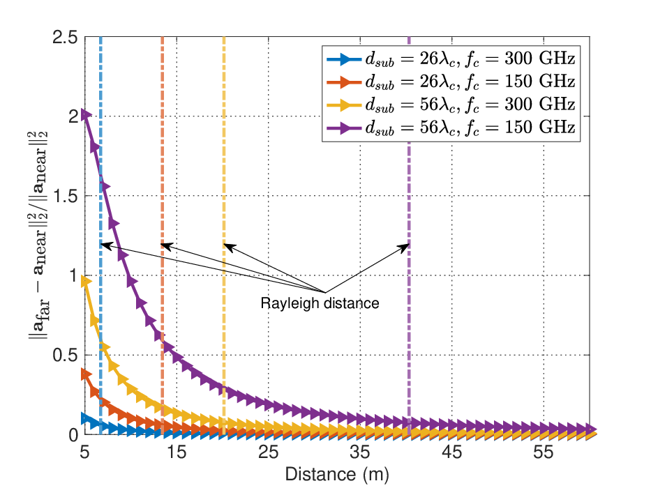
Although is small in THz systems, the massive number of AEs and the widely spaced SAs can still result in a quite large near-field region. Due to the limited coverage of THz wave, the far-field and near-field regions typically coexist. The portion can vary based on the specific system settings. For reference, in some typical THz UM-MIMO systems with planar AoSA is illustrated in Fig. 2.
In view of this, we study the general case where the channel consists of a mixture of far- and near-field paths, i.e., the hybrid-field condition. In addition, the considered non-uniform planar AoSA also represents a general class of array geometry for THz UM-MIMO systems. The method proposed in this work is thus applicable to a broad range of system settings.
II-B Hybrid-Field THz UM-MIMO Channel Model
Due to the limited scattering of the THz wave, the spatial-frequency channel between the BS and a specific UE can be characterized by the superposition of one LoS path and non-LoS paths [13], given by
| (4) |
where denotes the carrier frequency, while , , , , , and are respectively the path loss, azimuth AoA, elevation AoA, distance between the array and the RF source/scatterer, the array response vector, and the time delay of the -th path. In particular, , , and are measured with respect to the origin of the coordinate system, as shown in Fig. 1(a).
II-B1 Path Loss
In addition to the spread loss, the molecular absorption loss is non-negligible at the THz band. The path loss accounts for both of them. Assuming that denotes the LoS path and denotes the NLoS paths, then
| (5) |
where is the reflection coefficient, is the LoS path length, and is the molecular absorption coefficient [13]. For the LoS path, . For NLoS paths, is given by
| (6) |
where is the angle of incidence of the -th path, is the angle of refraction. Also, and are respectively the refractive index and the roughness coefficient of the reflecting material [13]. Due to the severe penetration of the diffused and diffracted rays at THz band, their contributions are negligible over only a few meters [4]. Therefore, similar to [13, 11], the NLoS path loss model takes into account the single-bounce reflected rays only.
II-B2 Array Response Vector
As mentioned before, the array response vector differs in the far- and near-field regions, which are determined by the Rayleigh distance , and is given by
| (7) |
For notational brevity, we first construct the array response matrix. Due to the spherical wavefront, each element of the near-field array response matrix depends on the exact distance between each AE and the RF source/scatterer. For the -th path, the position of the RF source/scatterer is , where is the unit-length vector in the AoA direction, given by . Therefore, the array response of the -th AE in the -th SA is given by
| (8) |
where is the speed of light. The near-field array response vector is . Due to the planar wavefront in the far-field region, the exact distance can be approximated by a linear function of the SA and AE indexes. Therefore, each element of the far-field array response matrix is given by
| Algorithm | Linear estimator (LE) | Non-linear estimator (NLE) |
| PGD | ||
| ADMM | ||
| OAMP |
| (9) |
where the term in the exponent is the linear approximation of the exact distance obtained by the first-order Taylor expansion. Afterwards, the relevant far-field array response vector can also be obtained by vectorization, i.e., .
In Fig. 2, we plot the accuracy of the far-field array response versus the distance , when , , , , and . Four curves with different SA spacings and carrier frequencies are drawn for comparison. Depending on the system settings, the portion of the far- and near-field regions vary. The Rayleigh distance is shown by a vertical line with the same color as the corresponding curve. We can see that the far-field array response is correct when is beyond the Rayleigh distance . However, the approximation is inappropriate in the near-field region where . In this case, the accurate near-field array response must be used.
II-B3 Sparse Channel Representation
For channel estimators based on sparse reconstruction, the fundamental assumption is that the spatial channel can be transformed to its sparse representation22 2 We introduce the sparse representation here only for ease of comparison with the benchmarks. Our proposal does not rely on the channel sparsity. in the form of , under an appropriate dictionary matrix . Since each SA in the planar AoSA is a UPA with identical geometry, we could design the overall dictionary matrix in an SA-by-SA manner. For far-field paths, the array response in (9) is a linear function of the AE index, and is insensitive to the distance . Therefore, for each SA, one can use the DFT-based dictionary to uniformly sample the AoAs and , which is constructed by the Kronecker product of two normalized DFT matrices of size [16]. The overall dictionary matrix is then with each component matrix . For near-field paths, the array response in (8) is a non-linear function of the AE index, and is sensitive to both the AoAs , and the distance . To handle this, the idea in previous works is to sample both the AoAs and the distance to construct a higher dimensional angle-distance domain dictionary matrix [14]. However, for the considered hybrid-field case, the optimal dictionary is dependent on the portion of the far-field and near-field paths. The state-of-the-art solution in the literature is to apply dictionary learning to optimize the dictionary matrix using site-specific data [16].
In our simulations, we adopt dictionary learning when comparing with the CS-based benchmarks since their performance is heavily affected by the quality of the sparse representation. Discussions on the details are deferred to Section V. For the proposed method and the other DL-based benchmarks, we simply adopt the DFT-based far-field dictionary since their performance does not rely on the channel sparsity.
II-C Problem Formulation
In the uplink channel estimation, the UEs transmit training pilots to the BS for time slots. We assume that orthogonal pilots are adopted and consider an arbitrary UE without loss of generality [13, 14]. The received pilot signal in the -th time slot at the BS is given by
| (10) | ||||
where denotes the digital combining matrix, is the analog combining matrix where the elements of each component vector satisfy the constant-modulus constraint, is the pilot symbol that is set as 1 for convenience, and is the additive white Gaussian noise (AWGN). Since the combining matrices cannot be optimally tuned without knowledge of the channel, we consider an arbitrary scenario where is set as identity and the analog phase shifts in are randomly picked from one-bit quantized angles, i.e., , to reduce the energy consumption [28]. The received pilot signal after time slots of the training pilot transmission is given by , where , and .
Since deep learning packages require real-valued inputs, we transform the system model into its equivalent form. Denoting , . , and
| (11) |
the equivalent real-valued system model is given by

| (12) |
The channel estimation aims to recover the channel representation from the measurement , with the knowledge of the measurement matrix . If available, the statistics of the noise can also be utilized to enhance the performance. In the following, we propose FPN-based algorithms to solve the problem. Notice that (12) is also relevant to the general linear inverse problems that are prevalent in the physical layer, e.g., detection and decoding [25]. The proposed method can also provide inspirations for DL-based solutions to these problems.
III FPNs for THz UM-MIMO Channel Estimation
III-A Preliminaries of Model-Driven DL
The measurement matrix will be singular, if the number of pilots is reduced. Prior information must be exploited in either the form of regularization or prior distribution to ensure robust estimation. The former formulates channel estimation as a regularized LS (RLS) problem, i.e., , where is a positive scalar and is a sparsity-inducing regularizer, e.g., the -norm. The RLS can be solved by proximal gradient descent (PGD) or alternating direction method of multipliers (ADMM) algorithms [39]. The latter formulates channel estimation as maximum a posteriori (MAP) or minimum mean squared error (MMSE) inference, which can be tackled by approximate message passing (AMP) and OAMP [17, 18]. Although these two categories of algorithms have distinct principles and purposes, their per-iteration update rules are similar in form. In particular, they can be divided into the linear estimator (LE) and the non-linear estimator (NLE), as listed in Table I. In the table, is the step size, the superscript is the -th iteration, denotes the proximal operator [39], is the LE matrix of OAMP, and denotes the NLE of OAMP. The last two will be detailed later in Section III-D. The LE enforces the estimation to be consistent with the received pilots, while the NLE ensures that the estimation agrees with the prior knowledge of the channel. The channel estimation algorithms can be interpreted as the fixed point iteration of the composition of the LE and the NLE, which can run an arbitrary number of iterations until convergence [40]. The estimated channel is then the stable state of the fixed point iteration, called the fixed point or equilibrium point.
The LE relies on the received pilot signals, which is known perfectly, and is easy to construct. However, the bottlenecks of the above algorithms all lie in the NLEs since their design requires prior knowledge of the channel, which is difficult to acquire. Hand-crafted regularizers or priors can only capture the rough information since they are limited by their analytical structure. For example, the dictionary matrix may not sparsify the channel well and can cause energy leakage effects. Similarly, the empirically chosen base distribution to model the prior can be mismatched with the true prior distribution.
One natural idea is to replace NLEs with neural networks and then learn to exploit the prior information of the channel from data, which becomes well-motivated in theory due to two seminal works [41, 42]. In [41], the authors found that the proximal operators in PGD and ADMM could be understood as MAP estimators of Gaussian denoising problems. In [42], the authors found that the NLEs in AMP, OAMP and related algorithms can also be interpreted as Gaussian noise denoisers. Deep neural networks, known as powerful denoisers, are thus well-suited to substitute the NLEs, which leads to the thriving of model-driven DL-based channel estimators [28, 29, 31].
III-B Motivations of FPNs
Model-driven DL-based, i.e., deep unfolding-based, estimators suffer from several systematic drawbacks, which make them unsuitable for THz UM-MIMO. In the sequel, we discuss these drawbacks and reveal the motivations of our proposal.
Deep unfolding-based estimators are constructed by first truncating a classical iterative algorithm to pre-defined and fixed layers, and then substituting each NLE in layer by a deep neural network parametrized by [28, 29, 31], as illustrated in Fig. 3. In layer , the LE is denoted by and the NLE is given by . The overall update in layer is the composition of the LE and the NLE, given by
| (13) |
The difference between specific works only lies in the choice of the base algorithm, which affects , and the choice of the neural network, which impacts . The training process can be described by an optimization problem, i.e.,
| (14) | ||||
where is the loss function, denotes the collection of trainable parameters, and denotes the ground-truth channel. The mapping defines an explicit neural network structure with truncated layers in forward propagation.
Nevertheless, the accustomed formulation of deep unfolding can give rise to several critical problems when it is applied to THz UM-MIMO channel estimation. First, it scales poorly with the UM-MIMO array. The required gradient in the training, i.e., backward, process of (14) is computed using the chain rule, i.e., step-by-step gradient, which involves tracking and storing all the intermediate states and causes a high space complexity of [43, 35]. For UM-MIMO systems with thousands of antennas and complicated channel conditions, the training cost is unaffordable. Second, the reliability is not guaranteed. Truncating the algorithm to layers breaks the convergent nature of classical iterative algorithms. The objective in (14) only minimizes the estimation accuracy of the final layer . Nonetheless, the intermediate state is not meaningful and tends to oscillate frequently [33]. Third, the complexity is high and not adaptive. Owing to the unreliable intermediate states, deep unfolding algorithms are not adaptive and must be run for the full layers, which causes excessive complexity. Lastly, the generalization ability is poor in simulations, which cannot handle the changeable channel conditions in THz UM-MIMO.
Given these systematic drawbacks, it is important to rethink the feasibility of the deep unfolding framework. Some previous works noticed the complexity issue mentioned above, and proposed reinforcement learning-based modules to realize early exit of the unfolding process [30, 44]. Nevertheless, the other issues still remain open, which motivates us to propose a new and general framework to solve all these problems and embed DL into iterative estimators in a theoretically sound manner.
III-C General Ideas of FPNs
As mentioned in Section III-A, the estimated channel with classical iterative algorithms is the stable state of the iteration, i.e., the fixed point defined by , where the subscript here indicates that the parameters of the NLEs are the same in each iteration. If we can construct a DL-involved mapping whose repeated application leads to a fixed point that corresponds to the estimated channel, then the merits of classical algorithms will be perfectly preserved. In addition, the powerful learning capability of deep neural networks can be exploited at the same time, having the best of both worlds. We refer to such framework as FPNs, which is formulated by
| (15) |
Let us first suppose that the fixed point exists and is also unique. We will discuss how to satisfy this assumption soon. Then, (15) defines a bi-level optimization problem, where the inner level requires computing the fixed point of the mapping , while the outer level is the minimization of the loss with respect to the parameters of the NLE neural network . This is drastically different from the constraint in (14) which prescribes an explicit neural network structure. On the contrary, the constraint in (15) is rather defining what one wants the DL-based mapping to achieve, other than providing an explicit structure, as shown in Fig. 3. For example, to get the fixed point , i.e., the estimated channel, given different pilot signals , may be executed for different numbers of times, with different computational graphs. FPNs thus belong to implicit DL [43], which can extend to an arbitrary number of iterations until convergence.
To tackle the bi-level problem (15), one common method is to compute the implicit gradient based on the implicit function theorem [43, 45], as given in the following proposition.
Proposition 1.
Given the fixed point equation and the loss function , the gradient of the loss with respect to is calculated by
| (16) |
Proof:
Please refer to Appendix A. ∎From (16), we observe that calculating the implicit gradient only requires the fixed point , without the need of storing any intermediate states . As a result, the memory complexity is only regardless of the number of executed iterations, which is drastically smaller in comparison to deep unfolding, i.e., . However, calculating the matrix inverse in (16) is very costly given the high dimension of the channel. We turn to the approximate gradient proposed in [35] to reduce the computational overhead, given by
| (17) |
This has been proved to be a descending direction of the loss under mild assumptions and achieved empirical success [35]. In addition, to realize (17) in the DL libraries, e.g., Pytorch, one only needs to modify a few lines of codes compared to the standard training procedure [35, Section III]. We refer to this as one-step gradient, as the backward process only depends on one addition application of at , regardless of how many iterations it takes to reach the fixed point .
With the low-cost training procedure at hand, the remaining problem is how to ensure that the fixed point exists and is unique, and how to find the fixed point efficiently. Before going on, we first introduce two key concepts.
Definition 2 (Lipschitz continuity).
A mapping is said Lipschitz continuous if there exists a constant such that
holds for any .
Definition 3 (Contraction).
A mapping is a contraction mapping if it is Lipschitz with constant .
The existence of the fixed point and an efficient way to find it can be ensured by fixed point theory [40]. As long as is a contraction mapping (no matter what detailed operations it contains), a simple repeated application of will make converge in linear rate to the unique fixed point . This can be formally stated in the following lemma.
Lemma 4 (Banach [40, Theorem 1.50]).
For any initial value , if the sequence is generated via the relationship and is a contraction mapping with Lipschitz constant , then converges to the unique fixed point of with a linear convergence rate .
The above lemma indicates that if one can train a contraction with DL-based components , then the convergence of FPNs to the unique fixed point in linear rate can be theoretically guaranteed. That is to say, we should control the Lipschitz constant of . Since the LEs of classical iterative algorithms are all linear functions of , their Lipschitz constants can be easily computed. Therefore, we only need to control the Lipschitz constant of the neural network component . Given the following lemma, we can work out the exact requirement of the neural network .
Lemma 5 ([46]).
The composition of an -Lipschitz and an -Lipschitz mapping is -Lipschitz.
The lemma above helps us identify the required Lipschitz constant of neural network to ensure the linear convergence. With such knowledge, we can control the Lipschitz constant of during the training process with many off-the-shelf methods [46]. Note that Lipschitz-continuous neural networks can also contribute to the adversarial robustness [46], which is beneficial to the superb out-of-distribution robustness of FPNs observed in the simulations in Section VI.
In the sequel, we present an example of the FPN-enhanced iterative channel estimator based on OAMP so as to illustrate the design guideline. Similar procedures can also be applied to enhance other iterative estimators, e.g., PGD and ADMM, which indicates the generality of the proposed FPNs.
III-D FPN-OAMP: Enhancing OAMP with FPNs
OAMP is an efficient compressed sensing algorithm to solve channel estimation problems, which consists of a de-correlated LE and a divergence-free NLE, as shown in Table I [18]. In the sequel, we present the specific design of the FPN-enhanced OAMP algorithm, i.e., FPN-OAMP.
III-D1 Linear Estimator
The LE of FPN-OAMP is similar to the original one in OAMP, given by
| (18) |
where is a de-correlated LE matrix. The matrix can be built upon the transpose and the pseudo-inverse of , or the linear minimum mean square error (LMMSE) matrix [18]. The first two do not depend on the noise statistics and are the same in each iteration, which match the FPN framework. While the last one is the optimal form, it depends on the noise statistics and requires computing a matrix inverse in each iteration, making it too complicated for UM-MIMO systems. We choose the pseudo-inverse LE due to its competitive performance and reasonable cost. The LE matrix is given by
| (19) |
where is the step size to guarantee that holds, such that the LE is de-correlated. That is, the elements of the NLE input error vector are mutually uncorrelated with zero-mean and identical variances [18].
III-D2 Non-linear Estimator
The NLE in FPN-OAMP ensures that the estimation is consistent with the prior knowledge of the channel. We replace the NLE in the original OAMP with neural networks to learn to exploit the prior knowledge from data. The NLE in FPN-OANP is given by
| (20) |
| (21) |
which is a neural network parametrized by . Specifically, is designed as a ResNet structure with three residual blocks (RBs) [47]. Before the RBs, is first reshaped into a tensor form of feature maps of size , each corresponding to an SA, and then passed through a convolution (Conv) layer to lift it to 64 feature maps. Each RB is formed by an identity mapping plus the compositions of Conv with 64 feature maps and ReLU activation function, as shown in Fig. 4. After the RBs, we apply two Conv layers with feature maps, and reshape the output into a vector with the same size as . We adopt layer normalization in each RB for more stable training [48], which is suitable for recurrent neural networks, and so as the FPNs.
There are two takeaways in the design of . First, since the planar AoSA is non-uniform, the relationship of the channel between inter-SA and intra-SA antennas are different. Therefore, one should separate the SA channels into different feature maps, other than using the channel of the whole array as the input to the neural network. Second, the residual links are important to make the NLE approximately divergence-free. With such design, the statistical properties of the original OAMP still hold well for FPN-OAMP [49]. By contrast, the NLE without residual links offers much worse performance.
FPN-OAMP is summarized in Algorithm 1, which is designed as the fixed point iteration of the contraction mapping . We then discuss the key theoretical properties of FPN-OAMP and the requirements on DL-based to ensure that the mapping is a contraction.
III-E Key Theoretical Properties
III-E1 Representational Power
The proposed FPNs restrict the parameters of the DL-based NLE to be identical in each iteration in order to match the requirements of fixed point iteration. This initially seems a drawback over existing deep unfolding methods, which do not require the parameters to be identical and generally use a different set of parameters for each layer, i.e., . Nevertheless, the representational power of FPNs has no notable loss compared to deep unfolding due to the proposition below, even though they are much cheaper to train [43]. Simulations in Section V also confirm the advantages of FPNs over deep unfolding.
Proposition 6 ([43, Theorem 3]).
For a -layer deep unfolded network with different parameters per layer, there exist FPNs that can represent the same network with equivalent depth.
III-E2 Linear Convergence Rate
We provide the proof for the linear convergence of FPN-OAMP to a unique fixed point and the requirement on the DL-based NLE .
Theorem 7.
The sequence generated by FPN-OAMP updates converges to a unique fixed point with linear convergence rate if the DL-based NLE is a contraction with Lipschitz constant .
Proof:
Please refer to Appendix B. ∎We discuss how to train the DL-based NLE as a contraction mapping in Section III-F. The linear convergence property ensures the reliability and efficiency of FPN-OAMP, which is not available for existing deep unfolded methods. In addition, since the inference process of FPNs is to find the fixed point of a contraction, many advanced algorithms for this purpose, e.g., Anderson acceleration [40], can be adopted to potentially reach even super-linear convergence.
III-E3 Adaptive Accuracy-Complexity Tradeoff
As a corollary, the contraction property of FPN-OAMP further indicates that the gap between and is monotonically decreasing, according to the definition of Lipschitz continuity. This indicates that intermediate states of FPN-OAMP will be closer to the fixed point as the fixed point iteration goes. This provides a user-defined tradeoff between complexity and accuracy, which is valuable in practical deployment.
Corollary 8.
Given the sequence generated by FPN-OAMP updates with Lipschitz constant and fixed point , then holds.
III-F Offline Training and Online Self-Adaptation
The loss function we use, i.e., , is the weighted sum of two different terms, given by
| (22) |
where is the supervised main loss, is the unsupervised auxiliary loss, and is the hyper-parameter balancing these two terms. For both the main and auxiliary loss functions we utilize the normalized mean absolute error (NMAE) criteria, since it results in better performance and robustness compared to the normalized mean squared error (NMSE) loss according to the analysis in [50]. The expressions of the two terms are given in (20) on the top of the page. We let and denote a batch of estimated/ground-truth channels, while and denote a specific sample in that batch.
The offline training process is standard despite the use of the one-step gradient instead of the step-by-step gradient of the chain rule. In addition, we append a safeguarding step to ensure that the DL-based NLE, i.e., , in FPN-OAMP is contractive by checking the approximate Lipschitz constant over the current batch of data after each weight update, i.e.,
| (23) |
where denotes a small random perturbation. If is found, i.e., the contraction property does not hold, we normalize the weight according to , similar to [1]. Nevertheless, this is almost never violated in our experiments, indicating that the training process itself encourages the contraction property.
Although FPN-OAMP can directly generalize to almost all the tested distribution shifts in Section VI, it is still important to design an online self-adaptation scheme in case that direct generalization fails. Our scheme is inspired by [51] with two steps. First, include an unsupervised auxiliary loss at the offline training stage. Second, at the online deployment stage, if potential performance drop is detected33 3 In our recent work [49], we propose a preliminary method to realize this goal. However, detailed discussion on this is out of the scope of this paper. , fine-tune the model based on the offline-trained parameters using the auxiliary loss for the one particular received pilot signal . The overhead of one iteration of the online fine-tuning is roughly equal to doing one additional forward propagation, which is quite cheap. In practice, we find that around 5 iterations of fine-tuning is often enough. Notice that the online self-adaptation is only a backup option, since direct generalization can already handle most cases of distribution shifts.
III-G Complexity Analysis
We analyze the complexity based on the real-valued system model (12). The complexity of the LE in FPN-OAMP is dominated by matrix-vector product, given by , because the LE matrix is the same in each iteration and can be pre-computed and cached44 4 Note that this does not mean the algorithms can only work with the pre-specified measurement matrix. In Section VI, we will show that the proposed FPN-OAMP trained with a single measurement matrix can directly generalize to a wide variety of measurement matrix conditions.. The complexity of the NLE in FPN-OAMP depends on the number of floating point operations (FLOPs) of the neural network, which is constant and denoted by . To reach an -optimal precision of the fixed point, FPN-OAMP requires only iterations due to linear convergence. The overall complexity is , which scales linearly with the number of antennas. To illustrate the complexity straightforwardly, we provide the running time in Section V.
IV Extension to Wideband Systems
In previous sections, we adopted the narrowband system model to better illustrate the ideas of the proposed algorithms. Nevertheless, in practice, to exploit the huge available bandwidth, THz UM-MIMO systems are likely to be operated in the wideband mode. We discuss how our proposed method can be readily extended in the following.
Consider a wideband THz UM-MIMO orthogonal frequency division multiplexing (OFDM) system55 5 Another promising alternative to OFDM is single-carrier frequency domain equalization [13], to which the proposed method can also be easily extended. with the same BS array as in Section II. We consider subcarriers over a bandwidth of at the center frequency . For an arbitrary UE, the real-valued equivalent of the received signal at the -th subcarrier, , can be obtained in a similar manner as the narrowband case based on (12), i.e.,
| (24) |
where is the subcarrier index at frequency , and is the measurement matrix defined in Section II. It is irrelevant to the subcarrier index since the analog combiner is shared across different subcarriers [7]. Similar to in the narrowband case, the channel vector at the -th subcarrier, i.e., , can be generated by replacing with in (4). However, the gaps among the carrier frequencies are fairly large owing to the huge available bandwidth at the THz band, making the array response fairly frequency-selective. Even for the same multipath component, the beam power can still vary considerably at different subcarriers, which leads to the spatial wideband effect, or beam squint effect [34]. As a result, the combining gain or the effective signal-to-noise-ratio (SNR) is also unequal across subcarriers given that the analog combiner is shared [13]. This renders a key difference between narrowband and wideband channels.
We discuss two possible approaches to extending the algorithmic framework to wideband THz systems.
IV-A Narrowband Dataset
The most direct way is to employ the narrowband FPN-OAMP algorithm (trained for the central frequency ) to solve the channel estimation problem at each subcarrier in a parallel manner. For practical implementation, this can be easily achieved by increasing the testing batch size to the number of subcarriers. This method directly reuses the narrowband estimator without retraining thanks to the strong generalization capability. This method ignores the correlation between different subcarriers. Nevertheless, the performance is still competitive thanks to the strong generalization ability.
IV-B Wideband Dataset
The second method also deals with the wideband channel estimation problem through parallel subproblems. The key difference is that the network is trained using the wideband dataset, which covers all subcarriers, by treating the narrowband channel at each subcarrier as a separate training sample. After training, the inference procedure is the same as above. This can exploit the correlation among different subcarriers during training to tackle beam squint.
V Simulation Results
V-A Simulation Setup
We first consider the narrowband systems, while extension to the wideband systems is discussed at the end of this section. The main system parameters and their values are listed in Table II [13]. To model the hybrid-field channel conditions, the scatterer distance is set as a uniformly distributed random variable, spanning both the far-field and near-field regions. We adopt the NMSE between the estimated and the ground-truth channel as the performance metric, which is averaged over the testing dataset. The following six benchmarks are compared:
| Parameter | Value |
|---|---|
| Number of SAs / RF chains | |
| Number of AEs per SA | |
| Total number of BS antennas | |
| Carrier frequency | GHz |
| AE spacing | m |
| SA spacing | m |
| Pilot length | |
| Under-sampling ratio | |
| Azimuth AoA | |
| Elevation AoA | |
| Angle of incidence | |
| Number of paths | |
| Rayleigh distance | m |
| LoS path length | m |
| NLoS scatterer distance () | m |
| Time delay of LoS path | nsec |
| Time delay of NLoS paths () | nsec |
| Molecular absorption coefficient | m-1 |
| Refractive index | |
| Roughness factor | m |
- •
LS: Least squares estimation.
- •
- •
OAMP: Bayesian estimation via OAMP algorithm with the LMMSE LE, and Bernoulli-Gaussian prior [18].
- •
FISTA: Sparse reconstruction-based method with the fast iterative soft thresholding algorithm [52].
- •
EM-GEC: Bayesian estimation via EM-assisted generalized expectation consistent signal recovery with Gaussian mixture prior [22].
- •
ISTA-Net+: state-of-the-art deep unfolding method based on the iterative soft thresholding algorithm [53, 31].
Figure 5: NMSE comparison at different SNR levels. Figure 6: NMSE at iteration/layer ( dB). 
Figure 7: NMSE at iteration/layer ( dB).
Both ISTA-Net+ and the proposed FPN-OAMP are implemented by using Pytorch and trained for 100 epochs using the Adam optimizer. We set in (22), and use a batch size of 128 and an initial learning rate of 0.001. The learning rate is reduced by half after every 30 epochs. The training, validation, and testing datasets respectively consist of 80000, 5000, and 5000 samples. The SNR levels of the training and validation samples are randomly drawn from 0 to 20 dB. We observe that mixed-SNR training only causes a small drop in performance compared to dedicated-SNR training. Therefore, only a single set of parameters is trained. Due to the limitation of deep unfolding methods, ISTA-Net+ should be truncated to a finite number of layers. When training and testing ISTA-Net+, we set this number as 15, since a further increase can offer only negligible gain. When training the FPN-OAMP, we set the error tolerance as 0.01 and the maximum number of iterations as 15 for fair comparison with ISTA-Net+. At the testing stage, one can run FPN-OAMP for an arbitrary number of iterations until convergence. The training of FPN-OAMP takes only 50 minutes to complete and consumes less than 1.5 GB of memory on Nvidia A40 GPU.
We then introduce the choice of the dictionary . For deep learning based methods (i.e., ISTA-Net+ and FPN-OAMP), we adopt the DFT-based dictionary as introduced in Section III. For other benchmarks where the quality of the sparse representation is important, we resort to dictionary learning to enhance their performance [16]. The dictionary is obtained by an -sparse coding problem over the training dataset, i.e.,
| (25) |
where is the constraint set of the dictionary, i.e., , is the number of samples, and is a hyper-parameter [16]. In the objective, is the real-valued equivalent of the spatial channel . To solve the problem efficiently, we use the algorithm proposed in [54].
V-B Superior In-Distribution Performance
In Fig. 7, we present the NMSE comparison at different SNR levels. It demonstrates that our proposed FPN-OAMP outperforms all five benchmarks by a large margin. Compared with its base algorithm OAMP, the performance gain of FPN-OAMP is as large as 10 dB. This indicates that the CNN components of FPN-OAMP can effectively extract and exploit the structures of the complicated hybrid-field THz UM-MIMO channel. It is worth noting that, although we have augmented the CS-based benchmarks with dictionary learning, their performance still has a notable gap compared to DL-based ones. In addition, FPN-OAMP always outperforms the deep unfolding method, ISTA-Net+.
In Figs. 7 and 7, we compare the NMSE evaluated at different numbers of iterations/layers66 6 The term iteration is used when the algorithm we refer to can extend to an arbitrary depth, e.g., FPN-OAMP. By contrast, the term layer is adopted when the algorithm is truncated to a pre-defined and fixed depth, e.g., ISTA-Net+. , when the SNR is 5 dB and 15 dB, respectively. LS and OMP are not plotted since they do not produce intermediate results. In both cases, the proposed FPN-OAMP converges rapidly within 5 iterations. Furthermore, the performance of FPN-OAMP at the second iteration is already better than the final performance of all benchmarks. It is also observed that the accuracy of all methods, except ISTA-Net+, increases consistently with the number of iterations. The instability of ISTA-Net+ is mainly because it is truncated to a fixed number of layers, and only the final performance is optimized during training, with no control of the intermediate states. Due to such instability, to maintain competitive performance, ISTA-Net+ must use a fixed number of layers during both training and testing. By contrast, the proposed FPN-OAMP is adaptive in the number of iterations and has much more stable performance.
V-C Linear Convergence Rate
In Fig. 10, we evaluate the convergence of the proposed FPN-OAMP in terms of fixed point residual (left) and NMSE (right). Fixed point residual is given by . In the left figure, the fixed point is obtained by running FPN-OAMP for 200 iterations, well beyond that during training, i.e., 15 iterations. The curves are all linear before reaching convergence, which verifies the linear convergence rate proved in Theorem 7, and also justifies the safeguarding strategy in Section III-F. We also observe that the fixed point residual is monotonically decreasing, which agrees with Corollary 8. This eliminates the need of tricky stopping criteria. The difference norm or the running time budget can serve as good stopping criteria with theoretical support. In the right plot, it is observed that the NMSE converges after 2-5 iterations. The number of iterations required is slightly larger at higher SNR levels. We run the algorithm for a much larger number of iterations compared with the training stage, to confirm that it can extend to an arbitrary number of iterations.
V-D Adaptive Accuracy-Complexity Tradeoff
In Fig. 10, we compare the NMSE versus the running time when the SNR is 5 dB. The CPU running time is tested on Intel Core i7-9750H, while the GPU time is tested on Nvidia A40 GPU. The recorded running time contains only the online inference stage, while the time consumption of the offline stage, e.g., dictionary learning and DL training, is not included. As can be seen, the proposed FPN-OAMP always costs the least time to converge — only a few milliseconds even when tested on CPU. The per-iteration running time of FPN-OAMP is as low as that of the first-order optimization method FISTA, but it converges much faster with far better performance. Additionally, it is observed that, for any given running time budget, FPN-OAMP can always achieve a significantly better performance compared with all benchmarks. Furthermore, unlike deep unfolding methods, e.g., ISTA-Net+, which requires a fixed number of layers and therefore a fixed time budget, the running time of FPN-OAMP is adaptive. By adjusting the error tolerance or the running time budget, a user-defined tradeoff between complexity and accuracy can be readily achieved. This unique advantage is very important since the latency requirement and the computational capability may often vary in practical deployment.
V-E Extension to Wideband Systems
In Fig. 10, we compare the NMSE performance at different SNR levels for the wideband case. Besides the settings in Section V-A, the wideband system utilizes OFDM modulation with bandwidth GHz and subcarriers [13]. We adopt the HITRAN database to generate the frequency-dependent molecular absorption loss [11, 55]. For FPN-OAMP with the narrowband dataset, we directly utilize the same narrowband channel estimator at the center frequency . For the wideband dataset-based approaches, we train the network using the same mixed-SNR training strategy as in Section V-A. Simulation results show that both the narrowband and wideband variants of FPN-OAMP can significantly outperform ISTA-Net+. In addition, we observe that the narrowband variant is directly applicable to the wideband systems without notable performance loss, which demonstrates the strong generalization capability of FPN-OAMP over different frequency bands, even with the existence of beam squint.
VI Robust Out-of-Distribution Performance
Distribution shifts, i.e., the case where the distributions of the training and testing data differ, are prevalent in practical deployments and may cause serious performance degradations for DL-based channel estimators. This is the notorious out-of-distribution (OoD) problem. The distribution shifts related to channel estimation can be grouped as
- •
Noise distribution shifts in ,
- •
Channel distribution shifts in ,
- •
Measurement distribution shifts in .
With extensive simulations, we show the strong generalization capability of FPN-OAMP to all these distribution shifts. For the rare cases where direct generalization fails, we verify the effectiveness of the online self-adaptation scheme.
In the sequel, the source distribution by default refers to the same simulation setup described in Section V-A. In the tables below, we only list the particular configuration that is different in the source and target distributions. The rest configurations are kept unchanged. By in-distribution, we refer to the case where the model is trained and tested both on the target distribution. The training procedure on the target distribution dataset is exactly the same as that described in Section V-A. By OoD, we mean that the model is trained on the source distribution but tested on the target distribution. The performance is also averaged over 5000 testing samples.
VI-A Noise Distribution Shifts
In the first two rows of Table III, we study the influence of noise level shifts. For noise levels that are either lower or higher than the training configuration, the OoD performance is close to the in-distribution one. This demonstrates that the proposed FPN-OAMP is robust in face of noise level shifts, although it does not use any information of the noise statistics. Besides, we can further reduce the performance loss by enlarging the training SNR range based on practical needs.
In the third row of Table III, we examine the noise type shifts. We adopt the -stable distribution to model the impulsive noise [56, 57], which is defined by the stability parameter , the skewness parameter , and the dispersion parameter . Since the -stable noise has no limited variance, the normal SNR definition becomes invalid. We alternatively use the generalized SNR (GSNR) defined as the ratio of the signal power and the dispersion parameter [56]. For evaluation, we let , , and set as such that the GSNR equals 15 dB. The result shows that the FPN-OAMP model trained with AWGN can directly generalize to the impulsive noise case.
VI-B Channel Distribution Shifts
In Table IV, we present the OoD generalization performance of the proposed FPN-OAMP under channel distribution shifts. The results in this table are all tested when the SNR is 15 dB, and the noise distribution type is AWGN.
In the first row, we consider the influence of LoS blockage, which may frequently occur in THz UM-MIMO systems due to the high penetration loss [3]. The channels in the source distribution all consist of one LoS and four NLoS paths, while the channels in the target distribution only consist of four NLoS paths, where the NLoS scatterer distance follows m. The result shows that the performance drop is less than 0.2 dB, suggesting that LoS blockage almost has no negative effect on our proposed FPN-OAMP.
In the second and third rows, we check the effect of the number of paths. The results suggest that breaking away from the original number of paths will cause nearly no detriment to the performance of FPN-OAMP.
In the fourth and fifth rows, we study the influence of field mismatch. To model the near-field only channel, we set the source/scatterer distance as m, which is within the Rayleigh distance. We instead set the distance beyond the Rayleigh distance, as m, to model the far-field only channel. The performance drop is smaller than 0.1 dB, again demonstrating the robustness of FPN-OAMP.
| Source | Target | In-distribution | OoD NMSE |
| distribution | distribution | NMSE | (w/o self-ada.) |
| dB | dB | 5.44 dB | 5.34 dB |
| dB | dB | 24.85 dB | 24.27 dB |
| AWGN | Impulsive noise | 19.97 dB | 19.57 dB |
| Source | Target | In-distribution | OoD NMSE |
|---|---|---|---|
| distribution | distribution | NMSE | (w/o self-ada.) |
| LoS & NLoS | LoS blockage | 19.99 dB | 19.81 dB |
| paths | paths | 21.10 dB | 20.96 dB |
| paths | paths | 18.39 dB | 18.22 dB |
| Hybrid-field | Near-field only | 19.31 dB | 19.25 dB |
| Hybrid-field | Far-field only | 19.43 dB | 19.40 dB |
| 19.44 dB | 19.42 dB | ||
| 19.43 dB | 19.42 dB | ||
| 19.39 dB | 19.31 dB | ||
| 19.94 dB | 19.59 dB | ||
| Perfect array | Miscalibrated array | 19.00 dB | 18.90 dB |
From the sixth to the eighth row, we show the effects of SA spacing mismatch. In the source distribution, the SA spacing is set as , while in the target distribution, it is changed to , respectively. The change in array geometry will also affect the Rayleigh distance, which becomes 1.44 m, 10.40 m, and 33.12 m, respectively. The array geometry mismatch can also causes the side effect of field mismatch. In such a complicated OoD setting, the performance of FPN-OAMP is still robust. We further study the effect of mismatched AE spacing. As [3] pointed out, if plasmonic-based antennas are adopted, the AE spacing can be much smaller than the conventional choice of . In view of this, in the target distribution, we set the AE spacing as . The OoD NMSE is very close to the in-distribution one, suggesting that FPN-OAMP is also robust to AE spacing mismatch.
In the last row, we check the effects of array uncertainty. We follow [16] and focus on antenna gain miscalibration. For a perfect array, the antenna gains are equal. For miscalibrated array, 20% (205) randomly picked antennas are set as times the normal antenna gain with , while the rest 80% (819) antennas remain unchanged. The result suggests that FPN-OAMP is robust to array uncertainty.
VI-C Measurement Distribution Shifts
In Fig. 11 and Table V, we present the OoD generalization and/or self-adaptation performance of FPN-OAMP under measurement distribution shifts. The results are all tested when the SNR is 15 dB, and the noise distribution type is AWGN. Recall that the measurement matrix is determined by the pilot combiners , and the dictionary , as in Section II.
Since ISTA-Net+ and FPN-OAMP are both trained using a single realization of the random measurement matrix, it is important to examine whether the trained model can directly generalize to other different realizations. In Fig. 11, we present the cumulative distribution function (CDF) of the performance of such kind of OoD generalization when the under-sampling ratio is fixed as 50%. To plot the CDF, the model is tested using 1000 realizations of the measurement matrix that are different from the one used in the training stage. For each realization of the measurement matrix, the NMSE performance is averaged over 5000 testing samples. As a reference, we also plot a vertical line to show the in-distribution performance. It can be observed that the OoD performance drop of ISTA-Net+ can be as large as 1 dB. By contrast, the performance drop for the proposed FPN-OAMP is almost negligible.
In the first three rows of Table V, we examine the mismatch in the under-sampling ratio , which is affected by the pilot length . In the source distribution, the under-sampling ratio is set as 50%, while in the target distribution, it is changed to 70%, 30%, and 10%, respectively. We find that when is enlarged to 70%, the OoD performance remains unaffected. By contrast, when is decreased to 30% and 10%, the OoD performance drops drastically. These results suggest that FPN-OAMP can handle more received pilots but cannot directly generalize to the case where fewer pilots are transmitted than expected. In addition, we find that online self-adaptation can close 91% and 98% of the performance gap caused by the lower under-sampling ratios for the cases of and , respectively, demonstrating its effectiveness. Note that self-adaptation is mainly intended to handle abrupt changes in the environment. Doing this for every testing sample is not economical. If compatibility with different pilot length is required, one can train FPN-OAMP with the lowest allowed pilot length, since the model can generalize to the cases where more pilots are transmitted.
| Source | Target | In-dist. | OoD NMSE | OoD NMSE |
| dist. | dist. | NMSE | (w/o self-ada.) | (w/ self-ada.) |
| 20.62 dB | 20.62 dB | unnecessary | ||
| 14.86 dB | 7.05 dB | 13.16 dB | ||
| 7.62 dB | 0.92 dB | 6.28 dB | ||
| One-bit | Infinite-res. | 21.93 dB | 21.79 dB | unnecessary |
In the last row of Table V, we further study how the shift in the resolution of the pilot combiner affects the performance of FPN-OAMP. In the source distribution, the elements of the pilot combiner are picked from one-bit quantized angles, while in the target distribution, they are instead drawn from infinite-resolution angles. The result shows that pilot combiner resolution shift causes almost no OoD performance drop.
VII Conclusions
In this paper, we proposed FPNs, a unified and theoretically sound framework, to design scalable, low-complexity, adaptive, and robust DL-based channel estimation algorithms for THz UM-MIMO systems. The unique benefits of FPNs over the prevailing deep unfolding methods are established with firm theoretical supports. In addition to the general framework, a specific FPN-enhanced algorithm based on OAMP, i.e., FPN-OAMP, is also proposed. Extensive simulation results in a typical hybrid-field THz UM-MIMO system with planar AoSA are presented to demonstrate the significant gains of the proposed method in terms of various key performance indicators. Furthermore, FPN-OAMP exhibits strong robustness to distribution shifts and can directly generalize or self-adapt to a wide range of out-of-distribution scenarios, which makes it an ideal candidate for practical deployment.
Appendix A Proof of Proposition 1
The fixed point equation is , where can be viewed as an implicit function related to . We denote as when we treat it as an implicit function. By implicitly differentiating both sides with respect to , we get
| (26) |
where the second equality is due to the chain rule. Rearranging the terms above, we reach that
| (27) |
By using the chain rule again, we have the desired result, i.e.,
| (28) |
Appendix B Proof of Theorem 7
We begin by showing that the Lipschitz constant of the LE in FPN-OAMP, i.e., , equals 1. Since is an affine mapping, its Lipschitz constant is the spectral norm, i.e., the largest singular value, of the matrix , given by , where denotes the -th largest eigenvalue of a matrix. Because the non-zero eigenvalues of and are the same, the eigenvalues of equal either 0 or 1. Therefore, we can obtain that the Lipschitz constant of the LE equals 1. According to Lemma 5, the Lipschitz constant of is the same as that of , i.e., . Further applying Lemma 4 yields the desired result.
References
- [1] W. Yu, Y. Shen, H. He, X. Yu, J. Zhang, and K. B. Letaief, “Hybrid far- and near-field channel estimation for THz ultra-massive MIMO via fixed point networks,” in Proc. IEEE Global Commun. Conf. (GLOBECOM), Rio de Janeiro, Brazil, Dec. 2022.
- [2] T. S. Rappaport, Y. Xing, O. Kanhere, S. Ju, A. Madanayake, S. Mandal, A. Alkhateeb, and G. C. Trichopoulos, “Wireless communications and applications above 100 GHz: Opportunities and challenges for 6G and beyond,” IEEE Access, vol. 7, pp. 78 729–78 757, Jun. 2019.
- [3] H. Sarieddeen, M.-S. Alouini, and T. Y. Al-Naffouri, “An overview of signal processing techniques for terahertz communications,” Proc. IEEE, vol. 109, no. 10, pp. 1628–1665, Oct. 2021.
- [4] I. F. Akyildiz, C. Han, Z. Hu, S. Nie, and J. M. Jornet, “Terahertz band communication: An old problem revisited and research directions for the next decade,” IEEE Trans. Commun., vol. 70, no. 6, pp. 4250–4285, Jun. 2022.
- [5] C. Chaccour, M. N. Soorki, W. Saad, M. Bennis, and P. Popovski, “Can terahertz provide high-rate reliable low-latency communications for wireless VR?” IEEE Internet Things J., vol. 9, no. 12, pp. 9712–9729, Jun. 2022.
- [6] K. B. Letaief, Y. Shi, J. Lu, and J. Lu, “Edge artificial intelligence for 6G: Vision, enabling technologies, and applications,” IEEE J. Sel. Areas Commun., vol. 40, no. 1, pp. 5–36, Jan. 2022.
- [7] J. Zhang, X. Yu, and K. B. Letaief, “Hybrid beamforming for 5G and beyond millimeter-wave systems: A holistic view,” IEEE Open J. Commun. Soc., vol. 1, pp. 77–91, Jan. 2020.
- [8] B. Ning, Z. Tian, W. Mei, Z. Chen, C. Han, S. Li, J. Yuan, and R. Zhang, “Beamforming technologies for ultra-massive MIMO in terahertz communications,” IEEE Open J. Commun. Soc., vol. 4, pp. 614–658, Feb. 2023.
- [9] C. Lin and G. Y. Li, “Terahertz communications: An array-of-subarrays solution,” IEEE Commun. Mag., vol. 54, no. 12, pp. 124–131, Dec. 2016.
- [10] Y. Huang, Y. Li, H. Ren, J. Lu, and W. Zhang, “Multi-panel MIMO in 5G,” IEEE Commun. Mag., vol. 56, no. 3, pp. 56–61, Mar. 2018.
- [11] S. Tarboush et al., “TeraMIMO: A channel simulator for wideband ultra-massive MIMO terahertz communications,” IEEE Trans. Veh. Technol., vol. 70, no. 12, pp. 12 325–12 341, Dec. 2021.
- [12] J. W. Choi, B. Shim, Y. Ding, B. Rao, and D. I. Kim, “Compressed sensing for wireless communications: Useful tips and tricks,” IEEE Commun. Surv. Tut., vol. 19, no. 3, pp. 1527–1550, third quarter, 2017.
- [13] K. Dovelos, M. Matthaiou, H. Q. Ngo, and B. Bellalta, “Channel estimation and hybrid combining for wideband terahertz massive MIMO systems,” IEEE J. Sel. Areas Commun., vol. 39, no. 6, pp. 1604–1620, Jun. 2021.
- [14] M. Cui and L. Dai, “Channel estimation for extremely large-scale MIMO: Far-field or near-field?” IEEE Trans. Commun., vol. 70, no. 4, pp. 2663–2677, Apr. 2022.
- [15] X. Wei and L. Dai, “Channel estimation for extremely large-scale massive MIMO: Far-field, near-field, or hybrid-field?” IEEE Commun. Lett., vol. 26, no. 1, pp. 177–181, Jan. 2022.
- [16] Y. Ding and B. D. Rao, “Dictionary learning-based sparse channel representation and estimation for FDD massive MIMO systems,” IEEE Trans. Wireless Commun., vol. 17, no. 8, pp. 5437–5451, 2018.
- [17] D. L. Donoho, A. Maleki, and A. Montanari, “Message-passing algorithms for compressed sensing,” Proc. Nat. Acad. Sci., vol. 106, no. 45, pp. 18 914–18 919, Nov. 2009.
- [18] J. Ma and L. Ping, “Orthogonal AMP,” IEEE Access, vol. 5, pp. 2020–2033, Jan. 2017.
- [19] C.-K. Wen, S. Jin, K.-K. Wong, J.-C. Chen, and P. Ting, “Channel estimation for massive MIMO using Gaussian-mixture Bayesian learning,” IEEE Trans. Wireless Commun., vol. 14, no. 3, pp. 1356–1368, Mar. 2015.
- [20] S. Srivastava, A. Tripathi, N. Varshney, A. K. Jagannatham, and L. Hanzo, “Hybrid transceiver design for tera-hertz MIMO systems relying on Bayesian learning aided sparse channel estimation,” IEEE Trans. Wireless Commun., vol. 22, no. 4, pp. 2231–2245, Apr. 2023.
- [21] F. Bellili, F. Sohrabi, and W. Yu, “Generalized approximate message passing for massive MIMO mmwave channel estimation with Laplacian prior,” IEEE Trans. Commun., vol. 67, no. 5, pp. 3205–3219, Jan. 2019.
- [22] R. Wang, H. He, S. Jin, X. Wang, and X. Hou, “Channel estimation for millimeter wave massive MIMO systems with low-resolution ADCs,” in Proc. IEEE Int. Wkshp. Signal Process. Adv. Wireless Commun. (SPAWC), Cannes, France, Jul. 2019.
- [23] C. Huang, L. Liu, C. Yuen, and S. Sun, “Iterative channel estimation using LSE and sparse message passing for mmwave MIMO systems,” IEEE Trans. Signal Process., vol. 67, no. 1, pp. 245–259, Jan. 2019.
- [24] A. Liu, L. Lian, V. K. N. Lau, and X. Yuan, “Downlink channel estimation in multiuser massive MIMO with hidden Markovian sparsity,” IEEE Trans. Signal Process., vol. 66, no. 18, pp. 4796–4810, Sept. 2018.
- [25] H. He, S. Jin, C.-K. Wen, F. Gao, G. Y. Li, and Z. Xu, “Model-driven deep learning for physical layer communications,” IEEE Wireless Commun., vol. 26, no. 5, pp. 77–83, Oct. 2019.
- [26] P. Dong, H. Zhang, G. Y. Li, I. S. Gaspar, and N. NaderiAlizadeh, “Deep CNN-based channel estimation for mmwave massive MIMO systems,” IEEE J. Sel. Topics Signal Process., vol. 13, no. 5, pp. 989–1000, Sept. 2019.
- [27] Y. Chen, L. Yan, and C. Han, “Hybrid spherical- and planar-wave modeling and DCNN-powered estimation of terahertz ultra-massive MIMO channels,” IEEE Trans. Commun., vol. 69, no. 10, pp. 7063–7076, Oct. 2021.
- [28] H. He, C.-K. Wen, S. Jin, and G. Y. Li, “Deep learning-based channel estimation for beamspace mmWave massive MIMO systems,” IEEE Wireless Commun. Lett., vol. 7, no. 5, pp. 852–855, Oct. 2018.
- [29] H. He, R. Wang, W. Jin, S. Jin, C.-K. Wen, and G. Y. Li, “Beamspace channel estimation for wideband millimeter-wave MIMO: A model-driven unsupervised learning approach,” IEEE Trans. Wireless Commun., vol. 22, no. 3, pp. 1808–1822, Mar. 2023.
- [30] Q. Hu, S. Shi, Y. Cai, and G. Yu, “DDPG-driven deep-unfolding with adaptive depth for channel estimation with sparse Bayesian learning,” IEEE Trans. Signal Process., pp. 1–16, Sept. 2022.
- [31] W. Jin, H. He, C.-K. Wen, S. Jin, and G. Y. Li, “Adaptive channel estimation based on model-driven deep learning for wideband mmwave systems,” in Proc. IEEE Global Commun. Conf. (GLOBECOM), Madrid, Spain, Dec. 2021.
- [32] A. Balatsoukas-Stimming and C. Studer, “Deep unfolding for communications systems: A survey and some new directions,” in Proc. IEEE Int. Wkshp. Signal Process. Syst. (SiPS), Oct. 2019, pp. 266–271.
- [33] T. Chen, X. Chen, W. Chen, H. Heaton, J. Liu, Z. Wang, and W. Yin, “Learning to optimize: A primer and a benchmark,” J. Mach. Learn. Res., Jun. 2022.
- [34] B. Wang, F. Gao, S. Jin, H. Lin, and G. Y. Li, “Spatial- and frequency-wideband effects in millimeter-wave massive MIMO systems,” IEEE Trans. Signal Process., vol. 66, no. 13, pp. 3393–3406, Jul. 2018.
- [35] S. W. Fung, H. Heaton, Q. Li, D. McKenzie, S. Osher, and W. Yin, “JFB: Jacobian-free backpropagation for implicit models,” in Proc. Assoc. Adv. Artif. Intell. (AAAI), Virtual, Feb. 2022.
- [36] M. Cui, Z. Wu, Y. Lu, X. Wei, and L. Dai, “Near-field MIMO communications for 6G: Fundamentals, challenges, potentials, and future directions,” IEEE Commun. Mag., vol. 61, no. 1, pp. 40–46, Jan. 2023.
- [37] X. Ma, Z. Gao, F. Gao, and M. Di Renzo, “Model-driven deep learning based channel estimation and feedback for millimeter-wave massive hybrid MIMO systems,” IEEE J. Sel. Areas Commun., vol. 39, no. 8, pp. 2388–2406, Aug. 2021.
- [38] C. A. Balanis, Antenna theory: analysis and design. John wiley & sons, 2015.
- [39] S. Boyd et al., “Distributed optimization and statistical learning via the alternating direction method of multipliers,” Found. Trends Mach. Learn., vol. 3, no. 1, pp. 1–122, 2011.
- [40] H. H. Bauschke and P. L. Combettes, Convex analysis and monotone operator theory in Hilbert spaces (2nd edition). Springer, 2019.
- [41] S. V. Venkatakrishnan, C. A. Bouman, and B. Wohlberg, “Plug-and-play priors for model based reconstruction,” in Proc. IEEE Global Conf. Signal Inf. Process. (GlobalSIP), Austin, TX, USA, Dec. 2013, pp. 945–948.
- [42] C. A. Metzler, A. Maleki, and R. G. Baraniuk, “From denoising to compressed sensing,” IEEE Trans. Inf. Theory, vol. 62, no. 9, pp. 5117–5144, Sept. 2016.
- [43] S. Bai, J. Z. Kolter, and V. Koltun, “Deep equilibrium models,” in Proc. Adv. Neural Inf. Process. Syst. (NeurIPS), Vancouver, Canada, Dec. 2019.
- [44] W. Chen, B. Zhang, S. Jin, B. Ai, and Z. Zhong, “Solving sparse linear inverse problems in communication systems: A deep learning approach with adaptive depth,” IEEE J. Sel. Areas Commun., vol. 39, no. 1, pp. 4–17, Jan. 2021.
- [45] S. G. Krantz and H. R. Parks, The implicit function theorem: history, theory, and applications. Springer Science & Business Media, 2002.
- [46] H. Gouk, E. Frank, B. Pfahringer, and M. J. Cree, “Regularisation of neural networks by enforcing Lipschitz continuity,” Mach. Learn., vol. 110, no. 2, pp. 393–416, Dec. 2021.
- [47] K. He, X. Zhang, S. Ren, and J. Sun, “Deep residual learning for image recognition,” in Proc. IEEE Conf. Comput. Vis. Pattern Recog. (CVPR), Las Vegas, NV, USA, Jun. 2016.
- [48] J. L. Ba, J. R. Kiros, and G. E. Hinton, “Layer normalization,” in Proc. Adv. Neural Inf. Process. Syst. (NeurIPS), Barcelona, Spain, Dec. 2016.
- [49] W. Yu, H. He, X. Yu, S. Song, J. Zhang, and K. B. Letaief, “Blind performance prediction for deep learning based ultra-massive MIMO channel estimation,” in Proc. IEEE Int. Conf. Commun. (ICC), Rome, Italy, May 2023.
- [50] J. Qi, J. Du, S. M. Siniscalchi, X. Ma, and C.-H. Lee, “On mean absolute error for deep neural network based vector-to-vector regression,” IEEE Signal Process. Lett., vol. 27, pp. 1485–1489, Aug. 2020.
- [51] M. Z. Darestani, J. Liu, and R. Heckel, “Test-time training can close the natural distribution shift performance gap in deep learning based compressed sensing,” in Proc. Int. Conf. Mach. Learn. (ICML), Baltimore, MD, USA, Jul. 2022.
- [52] A. Beck and M. Teboulle, “A fast iterative shrinkage-thresholding algorithm for linear inverse problems,” SIAM J. Imaging Sci., vol. 2, no. 1, pp. 183–202, Feb. 2009.
- [53] J. Zhang and B. Ghanem, “ISTA-Net: Interpretable optimization-inspired deep network for image compressive sensing,” in Proc. IEEE/CVF Conf. Comput. Vis. Pattern Recognit. (CVPR), Salt Lake City, UT, USA, Jun. 2018.
- [54] J. Mairal, F. Bach, J. Ponce, and G. Sapiro, “Online dictionary learning for sparse coding,” in Proc. Int. Conf. Mach. Learn. (ICML), Jun. 2009.
- [55] I. E. Gordon et al., “The HITRAN2016 molecular spectroscopic database,” J. Quant. Spectrosc. Radiat. Transf., vol. 203, pp. 3–69, Dec. 2017.
- [56] C. L. Nikias and M. Shao, Signal processing with alpha-stable distributions and applications. Wiley-Interscience, 1995.
- [57] Y. Ma, Y. Shen, X. Yu, J. Zhang, S. H. Song, and K. B. Letaief, “Learn to communicate with neural calibration: Scalability and generalization,” IEEE Trans. Wireless Commun., vol. 21, no. 11, pp. 9947–9961, Nov. 2022.