Inclusion of heavy spin effects in the $ud\bar{b}\bar{b}$ $I(J^{P})=0(1^{-})$ four-quark channel in the Born-Oppenheimer approximation

Antiheavy-anitheavy-light-light tetraquarks have been studied extensively in recent years and received a lot of interest, in particular since there is experimental evidence that such states exist in the form of the $ud\bar{c}\bar{c}$ tetraquark $T_{cc}$ discovered by LHCb [1, 2].

On the theoretical side there is strong evidence that tetraquarks with flavor $ud\bar{b}\bar{b}$ and $I(J^{P})=0(1^{+})$ as well as with flavor $us\bar{b}\bar{b}$ and $J^{P}=1^{+}$ exist and are strong-interaction-stable, even though they have not been discovered by experiments yet. Within lattice QCD these systems were studied using antiheavy-antiheavy potentals and the Born-Oppenheimer approximation [3, 4, 5, 6] and also by full simulations, where Non Relativistic QCD is used for the heavy $\bar{b}$ quarks [7, 8, 11, 9, 10].

In Ref. [12] we predicted a $ud\bar{b}\bar{b}$ tetraquark resonance with quantum numbers $I(J^{P})=0(1^{-})$ around $17\,\text{MeV}$ above the $BB$ threshold. There we used a rather simple single channel Born-Oppenheimer setup, where effects due to the heavy quark spins are neglected. Since such effects could be of the order $\mathcal{O}(m_{B^{\ast}}-m_{B})=\mathcal{O}(45\,\text{MeV})$, it is essential to include these effects in a refined study of this tetraquark resonance, which we found in Ref. [12] close to the $BB$ threshold with a rather large width around $112\,\text{MeV}$. In this work, we carry out such a refined study by using an approach [6] developed in the context of the strong-interaction-stable $I(J^{P})=0(1^{+})$ tetraquark, which is also based on the Born-Oppenheimer approximation, but where two coupled channels, $BB$ and $B^{*}B^{*}$, are considered.

All calculations presented in this work are based on the Born-Oppenheimer approximation, which is composed of two major steps.

In the first step the heavy $\bar{b}$ quarks are treated as static and temporal correlation matrices of antiheavy-antiheavy-light-light interpolators are computed using standard methods from lattice QCD (see e.g. Ref. [5]). From these matrices corresponding antiheavy-antiheavy potentials can be extracted.

For isospin $I=0$ suitable interpolators generating $ud\bar{Q}\bar{Q}$ four-quark states are given by

where $\alpha,\beta,\gamma,\delta$ are spin indices, $a,b$ are color indices, $\vec{r}_{1}$ and $\vec{r}_{2}$ denote the positions of the static antiquarks $\bar{Q}$, $\mathbb{L}$ and $\mathbb{S}$ are $4\times 4$ spin matrices and $C=\gamma_{0}\gamma_{2}$ is the charge conjugation matrix. Since static spins do not appear in the Hamiltonian and are conserved quantities, it is important to couple the two static spins separately from the two light spins using $\mathbb{S}$ and $\mathbb{L}$, respectively. In the static limit there are only $4$ linearly independent heavy spin matrices $\mathbb{S}\in\{(\mathbb{1}+\gamma_{0})\gamma_{5},(\mathbb{1}+\gamma_{0})\gamma_{j}\}$, for which $O_{BB}$ does not vanish. For the light spin coupling there are $16$ possibilities, $\mathbb{L}\in\{(\mathbb{1}+\gamma_{0}),(\mathbb{1}+\gamma_{0})\gamma_{5},(\mathbb{1}+\gamma_{0})\gamma_{j},(\mathbb{1}+\gamma_{0})\gamma_{5}\gamma_{j}\}$. In total there are, thus, $4\times 16=64$ interpolators $O_{BB}$, which correspond to the $64$ possible combinations of pairs of $B$, $B^{*}$, $B_{0}$ and $B_{1}^{*}$ mesons.

For the Schrödinger equation discussed below we need potentials associated with pairs of $B$ and $B^{*}$ mesons, since channels containing a $B_{0}$ or a $B_{1}^{*}$ meson decouple. There are two such potentials, a strongly attractive potential $V_{5}$ corresponding to $\mathbb{L}=(\mathbb{1}+\gamma_{0})\gamma_{5}$ and a weakly repulsive potential $V_{j}$ corresponding to $\mathbb{L}\in\{(\mathbb{1}+\gamma_{0})\gamma_{j}\}$. Lattice QCD results extrapolated to physically light $u/d$ quark masses can be parameterized consistently by

with $\alpha_{5}=0.34_{-0.03}^{+0.03}$, $d_{5}=0.45_{-0.10}^{+0.12}\,\text{fm}$ [5] and $\alpha_{j}=-0.10\pm 0.07$, $d_{j}=(0.28\pm 0.017)\,\text{fm}$ [6]. The parameterizations are shown in Figure 1.

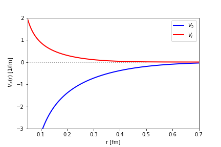
In the second step of the Born-Oppenheimer approximation the potentials $V_{5}$ and $V_{j}$ are used in a $16\times 16$ coupled channel Schrödinger equation, where each channel corresponds to a particular pair of $B$ and $B^{*}$ mesons. Effects due to the heavy quark spins are introduced via the mass splitting $m_{B^{*}}-m_{B}\approx 45\,\text{MeV}$ taken from experiments [13].

In detail, the Schrödinger equation for the relative coordinate of the two $\bar{b}$ quarks is given by

where, at large $\bar{b}\bar{b}$ separations $|\vec{r}|$, the 16 components of the wave function represent meson-meson pairs according to

(the indices $x,y,z$ refer to the orientation of the spins of the $B^{*}$ mesons). $H$ is the Hamilton operator,

with the meson masses $M=\text{diag}(m_{B},m_{B^{*}},m_{B^{*}},m_{B^{*}})$, the relative momentum of the the two $\bar{b}$ quarks and the reduced $b$ quark mass $\mu=m_{b}/2$. $H_{\text{int}}$ is a $16\times 16$ non-diagonal matrix containing the antiheavy-antiheavy potentials $V_{5}$ and $V_{j}$ computed in the first step. It is given by

where $V_{\text{diag}}$ is a diagonal $16\times 16$ matrix with entries $V_{5}$ or $V_{j}$ and $T$ is a $16\times 16$ transformation matrix, whose entries relate antiheavy-antiheavy potentials to meson-meson pairs. $T$ can be determined using Fierz identities, i.e. by expressing the fermion bilinears $(C\mathbb{L})_{\alpha\beta}u^{a}_{\alpha}d^{b}_{\beta}$ and $(C\mathbb{S})_{\gamma\delta}\bar{Q}^{a}_{\gamma}\bar{Q}^{b}_{\delta}$ in Eq. (1) in terms of the 16 components of the wave function defined in Eq. (4) (for details we refer to Ref. [6]). We note again that there is no coupling between channels with $B_{0}$ and/or $B_{1}^{*}$ mesons and the $16$ channels listed in Eq. (4).

One can show that both orbital angular momentum $L$ as well as total spin $S$ are conserved quantities. This allows to decompose the $16\times 16$ equation (3) into independent $1\times 1$ and $2\times 2$ equations with either symmetric or antisymmetric wave functions with respect to meson exchange. In this work we are exclusively interested to study a possibly existing resonance with $I(J^{P})=0(1^{-})$ predicted in Ref. [12], which has $L=1$ and $S=0$. Thus, we focus on the $2\times 2$ block representing $S=0$,

The potential matrix $V_{2\times 2}$ contains linear combinations of the potentials $V_{5}$ and $V_{j}$,

and entries of the 2-component wave function $\vec{\psi}_{2\times 2}$ can be interpreted according to

In this section we specialize the Schrödinger equation (7) to $L=1$. Moreover, we use standard techniques from scattering theory to implement boundary conditions, which define the T matrix (see e.g. Refs. [12, 14] for more detailed discussions).

We write each of the $2$ components of the wave function (9) as a superposition of an incoming partial wave proportional to $A_{\alpha}j_{1}(k_{\alpha}r)$, $\alpha\in\{BB,B^{*}B^{*}\}$, which is a solution of the free Schrödinger equation, and an emergent spherical wave proportional to $\chi_{\alpha}(k_{\alpha}r)/r$, i.e.

with $k=k_{BB}=\sqrt{2\mu(E-2m_{B})}$ and $k^{*}=k_{B^{*}B^{*}}=\sqrt{2\mu(E-2m_{B^{*}})}$. This leads to an ordinary differential equation for the radial coordinate $r$,

$A_{BB}$ and $A_{B^{*}B^{*}}$ reflect the composition of the incoming partial wave in terms of a $BB$ and a $B^{*}B^{*}$ meson pair, respectively. Moreover, the emergent wave is proportional to the corresponding scattering amplitude and $h_{1}^{(1)}(k_{\alpha}r)$ for large $r$. This allows to define the $2\times 2$ T matrix,

via

The first index of $t_{\alpha,\beta}$ refers to the incoming wave, the second index to the emergent wave. Poles of the T matrix indicate bound states (for $\text{Re}(E)<2m_{B}$) and resonances (for $\text{Re}(E)>2m_{B}$).

We used a standard fourth order Runge-Kutta method to solve the Schrödinger equation (11) for given complex energy $E$ and determined the corresponding T matrix (12) by comparing the wave function to the boundary conditions (13) and (14) at large $r$. Then we applied a Newton-Raphson root finding algorithm to $1/\det(\mbox{T}(E))$ to determine the poles of the T matrix in the complex energy plane.

When using the potentials (2), meson masses $m_{B}=5280\,\text{MeV}$, $m_{B^{*}}=5325\,\text{MeV}$ from the PDG [13] and $m_{b}=4977\,\text{MeV}$ from a quark model [15], we did not find a pole. In particular, there is no sign of the $I(J^{P})=0(1^{-})$ $ud\bar{b}\bar{b}$ tetraquark resonance predicted in Ref. [12] within a more basic single channel setup, where heavy spin effects and the mass splitting of the $B$ and the $B^{*}$ meson are neglected. The reason, why this resonance does not exist in the more realistic coupled channel setup introduced in this work, seems to be the competition between the attractive potential $V_{5}$ and the repulsive potential $V_{j}$. In the lighter $BB$ channel the potential is $(V_{5}+3V_{j})/4$ (see the upper left element of the potential matrix (8)), i.e. the attractive contribution is suppressed by the factor $1/4$, disfavoring the existence of a resonance. In the $B^{*}B^{*}$ channel the potential is $(3V_{5}+V_{j})/4$ (see the lower right element of the potential matrix (8)), i.e. the attractive component still dominates, but the potential is shifted upwards by $2(m_{B^{*}}-m_{B})=90\,\text{MeV}$, which is also not favorable concerning the formation of a resonance.

Our results presented in section 4 suggest that a $ud\bar{b}\bar{b}$ tetraquark resonance with $I(J^{P})=0(1^{-})$ does not exist. We note, however, that our approach, even though based on lattice QCD potentials, is not fully rigorous and resorts to certain approximations, e.g. the Born-Oppenheimer approximation. When comparing the mass of the strong-interaction-stable $ud\bar{b}\bar{b}$ tetraquark with $I(J^{P})=0(1^{+})$ obtained in the same approach [6] to results from recent full lattice QCD computations [7, 8, 11, 9, 10], there is a discrepancy in the binding energy, around $59\,\text{MeV}$ versus $100\ldots 150\,\text{MeV}$, which is not fully understood yet. Since full lattice QCD leads to stronger binding, it cannot be excluded, that the resonance exists in full QCD. Thus, to complement the results presented in this work, it would be interesting to also explore the $I(J^{P})=0(1^{-})$ sector using full lattice QCD with methods similar to those from Refs. [11, 17].

We acknowledge useful discussions with Pedro Bicudo, Lasse Müller, Martin Pflaumer and Jonas Scheunert. J.H. and M.W. acknowledge support by the Deutsche Forschungsgemeinschaft (DFG, German Research Foundation) – project number 457742095. A.Z.-S. acknowledges support by a Goethe Goes Global Scholarship. M.W. acknowledges support by the Heisenberg Programme of the Deutsche Forschungsgemeinschaft (DFG, German Research Foundation) – project number 399217702. Calculations were conducted on the GOETHE-HLR and on the FUCHS-CSC high-performance computers of the Frankfurt University. We would like to thank HPC-Hessen, funded by the State Ministry of Higher Education, Research and the Arts, for programming advice.

References

- [1] R. Aaij et al. [LHCb], Nature Phys. 18, no. 7, 751-754 (2022) [arXiv:2109.01038 [hep-ex]].
- [2] R. Aaij et al. [LHCb], Nature Commun. 13, no. 1, 3351 (2022) [arXiv:2109.01056 [hep-ex]].
- [3] P. Bicudo and M. Wagner, Phys. Rev. D 87, no. 11, 114511 (2013) [arXiv:1209.6274 [hep-ph]].
- [4] P. Bicudo, K. Cichy, A. Peters, B. Wagenbach and M. Wagner, Phys. Rev. D 92, no. 1, 014507 (2015) [arXiv:1505.00613 [hep-lat]].
- [5] P. Bicudo, K. Cichy, A. Peters and M. Wagner, Phys. Rev. D 93, no. 3, 034501 (2016) [arXiv:1510.03441 [hep-lat]].
- [6] P. Bicudo, J. Scheunert and M. Wagner, Phys. Rev. D 95, no. 3, 034502 (2017) [arXiv:1612.02758 [hep-lat]].
- [7] A. Francis, R. J. Hudspith, R. Lewis and K. Maltman, Phys. Rev. Lett. 118, 142001 (2017) [arXiv:1607.05214 [hep-lat]].
- [8] P. Junnarkar, N. Mathur and M. Padmanath, Phys. Rev. D 99, 034507 (2019) [arXiv:1810.12285 [hep-lat]].
- [9] R. J. Hudspith, B. Colquhoun, A. Francis, R. Lewis and K. Maltman, Phys. Rev. D 102, 114506 (2020) [arXiv:2006.14294 [hep-lat]].
- [10] P. Mohanta and S. Basak, Phys. Rev. D 102, 094516 (2020) [arXiv:2008.11146 [hep-lat]].
- [11] L. Leskovec, S. Meinel, M. Pflaumer and M. Wagner, Phys. Rev. D 100, 014503 (2019) [arXiv:1904.04197 [hep-lat]].
- [12] P. Bicudo, M. Cardoso, A. Peters, M. Pflaumer and M. Wagner, Phys. Rev. D 96, no. 5, 054510 (2017) [arXiv:1704.02383 [hep-lat]].
- [13] R. L. Workman et al. [Particle Data Group], PTEP 2022, 083C01 (2022).
- [14] P. Bicudo, N. Cardoso, L. Mueller and M. Wagner, Phys. Rev. D 103, no. 7, 074507 (2021) [arXiv:2008.05605 [hep-lat]].
- [15] S. Godfrey and N. Isgur, Phys. Rev. D 32, 189-231 (1985).
- [16] M. Neubert, Subnucl. Ser. 34, 98-165 (1997) [arXiv:hep-ph/9610266 [hep-ph]].
- [17] S. Meinel, M. Pflaumer and M. Wagner, Phys. Rev. D 106, 034507 (2022) [arXiv:2205.13982 [hep-lat]].