Sensitivity of strong lensing observations to dark matter substructure: a case study with Euclid2023Sensitivity of strong lensing observations to dark matter substructure: a case study with Euclid–References
Abstract
We introduce a machine learning method for estimating the sensitivity of strong lens observations to dark matter subhaloes in the lens. Our training data include elliptical power-law lenses, Hubble Deep Field sources, external shear, and noise and PSF for the Euclid VIS instrument. We set the concentration of the subhaloes using a - relation. We then estimate the dark matter subhalo sensitivity in simulated strong lens observations with depth and resolution resembling Euclid VIS images. We find that, with a detection threshold, per cent of pixels inside twice the Einstein radius are sensitive to subhaloes with a mass , per cent are sensitive to , and, the limit of sensitivity is found to be . Using our sensitivity maps and assuming CDM, we estimate that Euclid-like lenses will yield detectable subhaloes per lens in the entire sample, but this increases to per lens in the most sensitive lenses. Estimates are given in units of the inverse of the substructure mass fraction . Assuming , one in every lenses in general should yield a detection, or one in every three lenses in the most sensitive sample. From new strong lenses detected by Euclid, we expect new subhalo detections. We find that the expected number of detectable subhaloes in warm dark matter models only changes relative to cold dark matter for models which have already been ruled out, i.e., those with half-mode masses .
Keywords:
gravitational lensing: strong, dark matter1 Introduction
In cosmological models involving dark matter, galaxies reside in dark matter superstructures called haloes. Numerical simulations show that these haloes form hierarchically, merging with their neighbours and agglomerating smaller haloes (Springel et al. 2008). The distribution of these subhaloes in mass, called the subhalo mass function (SHMF) depends on the free-streaming properties of the dark matter, which is typically parametrised as a thermal relic dark matter particle mass, . In the canonical model, cold dark matter (CDM), the mass function is scale free and the number of objects at a given mass scales inversely with mass. For warmer models, i.e., smaller , we expect a suppression in dark matter structure formation for objects below a certain mass called the half mode mass, . Therefore, measuring the number and mass of dark matter subhaloes in galaxies provides a constraint on the dark matter model .
Strong gravitational lensing provides one method for measuring the distribution of dark matter subhaloes in the universe, amongst others (Koopmans 2005; Dalal & Kochanek 2002; Mao & Schneider 1998, e.g.). Subhaloes in the proximity of lensed images have a miniscule, but measurable effect on the local magnification. For point source objects like quasars, the effect of the subhalo is to produce anomalous flux ratios in the lensed images (Xu et al. 2015; Bradač et al. 2002). When the source is an extended object, a technique called gravitational imaging is used (Galan et al. 2022; Vernardos & Koopmans 2022; Vegetti & Koopmans 2009a). In gravitational imaging, small corrections to the potential, beyond that of the smooth lens galaxy, are found that improve the fit to the lensed images. The density field for this corrected potential can then reveal the locations and masses of subhaloes. Alternatively, the presence of substructures can be described analytically (He et al. 2022; Daylan et al. 2018, e.g.), or via the power-spectrum of mass density fluctuations (Chatterjee & Koopmans 2018, e.g.). So far, a small number of dark matter substructures have been detected (Hezaveh et al. 2016; Vegetti et al. 2012; Vegetti et al. 2010). In any CDM or WDM model, the number of detectable subhaloes expected in a typical lens with current instrumentation is of order unity, and so non-detections of subhaloes are common (Nightingale et al. 2022; Ritondale et al. 2019; Vegetti et al. 2014). It is therefore crucial to quantify the limits in subhalo mass of any non-detection in order to constrain the subhalo mass function.
Traditionally, the ability of a strong lens observation to detect subhaloes is quantified via the sensitivity function. In this procedure, the strong lens is modelled both with and without a subhalo in every pixel, over a range of subhalo masses (Ritondale et al. 2019; Vegetti et al. 2014). Bayesian model comparison then gives the difference in the log-evidence, between the models with and without subhaloes as a function of subhalo mass and position. By defining a threshold in at which a detection would be acceptable, one finds the minimum detectable subhalo mass in every pixel.
The nature of evidence calculations and the complexity of strong lens modelling mean that the sensitivity function is expensive to compute, often taking hundreds or thousands of CPU hours for a single observation. Calculating the sensitivity function is in fact the most expensive component of a gravitational imaging study. This is not necessarily an issue when the number of lenses available for study is small, as has been the case in the past. However, automations in lens finding and the advent of the sky-survey era means the number of known lenses is growing rapidly, and will continue to do so in the near future. The Euclid survey alone is predicted to yield more than new strong lenses, alongside similarly impressive contributions from the Dark Energy Survey (DES) and the Vera Rubin Observatory (Collett 2015, hereafter 8). It would be infeasible to conduct gravitational imaging studies on such a large number of objects with the current method, and so, we are motivated to find a more efficient method for calculating the sensitivity function.
In this paper, we demonstrate a new method for calculating the sensitivity to dark matter subhaloes in strong lens observations. Our method relies on machine learning, which is now widely used in strong lensing. This is especially true in lens finding, where convolutional neural networks (CNNs) are a natural choice (Wilde et al. 2022; Shu et al. 2022; Lanusse et al. 2018). Machine learning has also been used to estimate parameters for lens models (Gu et al. 2022; Schuldt et al. 2021; Chianese et al. 2020; Hezaveh et al. 2017). In our area of interest, detecting dark matter substructure, ML is also proving to be useful for replacing all or part of the traditional gravitational imaging pipeline. For example: Vernardos et al. 2020 show that a CNN can reliably estimate potential corrections in the lens; Wagner-Carena et al. 2022 use simulation-based inference to estimate the SHMF in a population of lenses; Ostdiek et al. 2022 and Diaz Rivero & Dvorkin 2020 show that direct detections with ML are possible in mock observations; and Coogan et al. 2020 develop a source light and lens potential modelling tool using ML.
Our approach for estimating subhalo sensitivity consists of two steps. In the first part, a CNN is trained to classify strong lens observations as either containing substructure or not. In the second step, the trained CNN is used to quantify the detectability of a single subhalo in every pixel, over a range of masses, in a given mock observation. In this way the method resembles the traditional approach, although without the expensive evidence calculations or forward modelling, these parts having effectively been replaced by the neural network. The mock observations we use in training are produced with realistic source brightness distributions from the Hubble Deep Field (Rafelski et al. 2015). They include elliptical power-law lenses and external shear, as well as a lens light subtraction.
The mock observations are intended to mimic the Euclid VIS instrument. The excellent angular resolution, seeing, and wide observing area of Euclid makes it particularly attractive for strong lensing studies and so we focus solely on Euclid VIS in this paper. However, the method we propose can readily be adapted to other instruments. A particular focus in this work is whether observations with the resolution of Euclid VIS will themselves be able to constrain the SHMF in a useful way. Subhalo sensitivity is primarily a function of the instrument angular resolution and signal to noise ratio (Despali et al. 2022). Hubble Space Telescope (HST) observations, at 0.04 arcsec resolution and total S/N are sensitive to subhaloes down to a mass of in the best cases, which allows to be constrained to roughly the same value (Ritondale et al. 2019). Constraints from other sources, including the abundance of Milky Way satellites, strong lensing flux ratios, gravitational imaging, and the Lyman- forest, have already ruled out a half mode mass above (Enzi et al. 2021; Nadler et al. 2021; Hsueh et al. 2020; Gilman et al. 2020). Even if the sheer number of Euclid VIS images cannot constrain the SHMF below the subhalo mass range of HST images, they will at least provide candidates for follow-up in higher resolution instruments that can. This is another motivation for this work, and for our interest in Euclid in general. If the sensitivity of images can be cheaply estimated a priori, then Euclid strong lenses can be ranked by sensitivity, and only the most promising candidates followed up in higher resolution instruments, e.g. the European Extremely Large Telescope (E-ELT).
The paper is organised as follows. In Section 2 we describe the procedure for producing mock strong lens observations. In Section 3 we detail the machine learning method and the training process. In Section 4 we present results from simulated Euclid images. In Section 5 we discuss our results and summarise our conclusions. Throughout this paper we assume a Planck 2015 cosmology with and (Planck Collaboration et al. 2016).
2 Simulated strong lens observations
A population of realistic Euclid strong lenses has already been simulated by 8. As such we follow the procedure therein wherever possible. In this section and the rest of the paper we refer to three types of data: training, testing, and evaluation. Each type uses the same method to produce the data, which we describe in this section, but their underlying model parameters are drawn from different distributions.
Evaluation data is that used to estimate sensitivity statistics for Euclid in our results. Training and testing data are used to train the network, and test its performance during training respectively. The evaluation data is sampled in a realistic way such that distributions of redshifts, Einstein radii, image configuration, signal to noise ratio, etc, are consistent with those expected in nature. These parameters are drawn from a simulation procedure, described below, and compiled in a catalogue. However, when we produce training and testing data we first resample these parameters from uniform distributions wherever possible. The intent is to prevent the neural network from specialising on specific cases that are more common in the physically sampled evaluation dataset. The training and testing data can be thought to cover, as uniformly as possible, all possible strong lenses, whereas the evaluation data are the actual strong lenses that we expect to observe with Euclid.
In training the network, complexity is added to the training data in stages. This section essentially describes the final stage, with previous stages either excluding some part, or using a simplified version of it. The details of these stages are given in Table 2.
2.1 Source galaxies
We begin with a population of sources to be lensed. For this we use the Hubble Deep Field (HDF) catalogue assembled by Rafelski et al. 2015. To obtain realistic statistics for substructure detectability it is vital to use complex source brightness distributions. This is because the local change in image surface brightness produced by substructure can be absorbed, to an extent, by a change in source surface brightness distribution. A CNN used to detect substructure must take this degeneracy into account, during training, to produce reliable results.
We denoise the sources using the method of Maturi 2017. The method uses Expectation Maximisation Principal Component Analysis (EMPCA) where images can be reconstructed from principal components. The lowest-order components fit the largest structures in the images, and the highest-order components fit only to the noise. By omitting some number of the largest principal components from the reconstruction, one obtains a denoised version of the original image. We divide the HDF images into six bins according to their angular size given in Rafelski et al. 2015. We then fit principal components separately in each bin. We determine the number of principal components to use in the reconstruction individually for each source. To do this, we compute a reduced chi-squared statistic between the reconstruction and the original noisy image, after adding each component. We stop adding principal components when the reduced chi-squared statistic no longer improves. The simplest sources, which are also the most numerous, require components for a good fit. The more complicated sources in the sample require up to principal components. The median number of components used in the entire sample is .
At selection time, the source redshift is resampled from a normal distribution centred on the original redshift in the HDF catalogue with a standard deviation . This helps the network generalise by smoothing out the underlying redshift distribution in the source catalogue, but keeps each source close to its original redshift when imaged. The angular size of the source is adjusted accordingly. The sources are themselves split into a training and testing set, with testing sources also used for the evaluation dataset. None of the sources used in our results were seen by the network during training. The final number of sources used is in the training set and in the testing and evaluation set.
2.2 Lens galaxies
For the lens galaxy we follow the same procedure as 8 and that reference should be consulted for details. We draw a velocity dispersion from the elliptical galaxy velocity dispersion function, in the range kms-1, and a lens redshift from the comoving volume function in the range . The lens is placed in a random angular position within the HDF field of view. For all HDF sources in the light cone behind the lens galaxy, the Einstein radius is calculated,
| (1) |
where is the speed of light and and are the angular diameter distances between the lens and the source, and the observer and the lens respectively. The source position is found relative to the centre of the lens galaxy and sources with are accepted.
The lens galaxy mass profile is a singular power-law ellipsoid. The dimensionless projected surface mass density, or convergence, is given by
| (2) |
where is the slope of the mass profile and is the lensing strength, where and is the axis ratio of the elliptical mass distribution (Tessore & Metcalf 2015). The axis ratio also defines the elliptical radius . The axis ratio is drawn from the axis ratio function for elliptical galaxies, as in 8, and can then be set from the already drawn velocity dispersion and Einstein radius. The slope of the mass profile is drawn from a normal distribution centred on (an isothermal slope) with standard deviation , approximately the distribution of slopes in lens galaxies (Bolton et al. 2008). We use a Sérsic profile for the lens galaxy surface brightness distribution with effective radius and magnitude drawn from the fundamental plane relation for elliptical galaxies. The Sérsic index is drawn from a scaling relation with the magnitude. Finally, to simulate the lensing effect of objects in the proximity of the main lens, we add external shear with a random angle and a random strength between and . This is typical of the shear strength found in strong lens observations (Bolton et al. 2008).
2.3 Subhaloes
In the training and testing data we add, with equal probability, either: zero subhaloes or; one to four subhaloes. The subhaloes are placed uniformly in a 6 arcsec 6 arcsec square centred on the lens galaxy. The largest lens used has arcsec, so the subhalo area always encloses . For the subhaloes we use an NFW density profile,
| (3) |
where is the radius in three dimensions, is the scale radius and is the normalisation, itself given by
| (4) |
where is the maximum circular velocity of particles in the subhalo and is a constant that relates to , the radius at which occurs,
| (5) |
Typically, the mass of the subhalo is taken to be the mass enclosed within the subhalo virial radius, prior to infall, which is labelled . In this work we instead use , the mass enclosed by . This more closely approximates the masses of subhaloes in simulations.
In training and testing the subhalo mass is drawn from a log-uniform distribution with limits . The concentration of the halo is typically set by the concentration mass relation given by Duffy et al. 2008. This relation for subhaloes is an extrapolation from that for larger haloes and may not be accurate at smaller masses, underestimating the concentration for subhaloes.
Instead, we set the concentration by applying a - relation obtained using the ShinUchuu simulation (Ishiyama & Ando 2020; Moliné et al. 2023),
| (6) |
where and 11 1 This version of the relation does not include a redshift dependence, although more recent versions do, see Moliné et al. 2023.. ShinUchuu is a higher resolution simulation with particles covering a 140 side length box, with resulting mass resolution of . Halo catalogues are available for public download22 2 http://www.skiesanduniverses.org and we use the results for and . We grouped subhaloes in bins of of equal size and obtained the mean of . Based on these results, we propose the - relation of Eq. 6. The parametrization works well for subhaloes with between km s-1 and km s-1 in host haloes with masses between and (its accuracy being better than 5 per cent at all values within this range).
In training and testing, we use the relation to set limits on a log-uniform distribution with , from which we draw a random . In evaluation, we convert the chosen to and take directly from Eq. 6 for the given . The NFW scale radius is then given in either case by Eq. 5. It is important to note that this relation produces subhaloes which are more concentrated than those used in previous gravitational imaging studies (Despali et al. 2018, e.g.). To make this clear, subhalo characteristics in our mass range are printed in Table 1.
| [kms-1] | [kpc] | ||||
|---|---|---|---|---|---|
2.4 Instrument characteristics
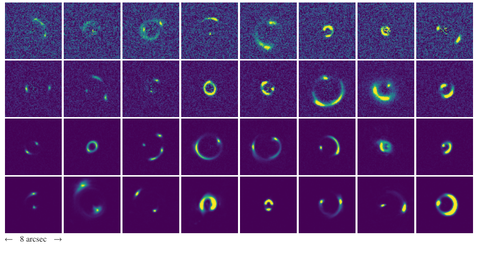
Using the described sampling procedure, we ran simulations to collect a large number of lens and source parameters. From this catalogue we then build the mock observations for training, testing and evaluation. The source surface brightness distribution is ray-traced through the mass model onto a grid with pixel size arcsec and a field of view of arcsec. To ensure an accurate source reconstruction in the image plane, we subsample each pixel with subpixels and use the mean over these subpixels. We add the lens light and convolve with a Gaussian PSF with FWHM arcsec. To this we add a uniform sky brightness of . We then compute the total expected counts for an observation with a zero-point of and an exposure time of s. The Euclid Wide Survey uses four exposures of s each, although due to gaps in the detector array and other technical considerations, the full survey area is only covered by three exposures (Euclid Collaboration et al. 2022). VIS technical details are taken from Vavrek et al. 2016 and Cropper et al. 2018. We use the expected counts in each pixel as the mean of a Poisson distribution from which we draw the actual total counts. Finally, we subtract the original Sérsic profile describing the lens light from this noisy image, leaving a Poisson-limited lens light subtraction. An example set of training observations are shown in Fig. 1.
3 Method
Our method comprises a number of steps. First, a neural network is trained on realistic mock observations that contain either zero or between one and four subhaloes, randomly placed in the image. The training is performed in stages where the complexity of the data is gradually increased and the model retrained. In the training stage, the observation parameters (Einstein radius, signal to noise ratio etc) are drawn uniformly from a wide range. Second, the trained model is used to predict the sensitivity in a second set of observations. In this stage, the observation parameters are drawn from realistic distributions, intended to match the expected population of Euclid strong lenses. For a given system in this population, we produce realisations of the same observation with a single subhalo, iterating over all subhalo positions and masses. For every position and mass, the trained network gives the probability that a subhalo is in the image. By defining a probability threshold at which a detection would be acceptable, we obtain the minimum detectable subhalo mass in each pixel. We repeat this process for a large number of mock Euclid observations to obtain our results.
3.1 Machine learning
We use the ResNet-50 architecture, commonly used in image classification tasks (He et al. 2015). ResNet is a residual convolutional neural network that utilises skip connections between network layers. These skip connections are designed to overcome the ‘vanishing gradient’ problem, and allow for the training of very deep networks. The architecture we use is unmodified from the original 50 layer implementation so we defer to the previous reference for details.
For a given image , the neural network returns the probability , that the image belongs to class . In our case there are only two classes, for an image with no substructure, and for an image with one or more substructures. We train using the Adam optimizer and minimise the cross-entropy between the network’s predictions and the truth. We use a batch size of . At training time, images are rescaled to the range , then randomly rotated, flipped and cropped to a size of arcsec, producing sized images from the original . The random crop ensures that the lens is not at the centre of the image, and improves training performance, without discarding any useful information given that all lenses have arcsec.
Training takes place in stages, with slight increases in the difficulty of the task at each stage. The stages are detailed in Table 2 and each stage’s data set consists of images. To achieve changes in the range of total signal to noise ratios, source magnitudes were changed from an initially constant in stage one, to a uniformly sampled range in stage three onwards. The lower limit of the subhalo mass range was moved down to in stage five from in stages one to four once it was found that a small number of lenses had sensitivity below this limit. External shear is added in stage four. At the start of each new stage we conduct a parameter search to find the optimum learning rate and the network starts with the converged parameters from the previous stage. As training progresses, the learning rate is multiplied by a decay factor of whenever the testing loss has not decreased for ten epochs. The network is assumed to have converged when three decreases in learning rate do not improve the test loss.
| Min. S/N | Min. | E.S. | Loss | Acc. | ||
|---|---|---|---|---|---|---|
| 1 | 0 or 1 | 0.307 | 0.867 | |||
| 2 | 0 or 1 | 0.575 | 0.673 | |||
| 3 | 0 or 1 | 0.610 | 0.638 | |||
| 4 | 0 or 1 | 0.641 | 0.599 | |||
| 5 | 0 or 1 | 0.678 | 0.538 | |||
| 6 | 0 or 1-4 | 0.658 | 0.569 |
3.2 Model performance
The performance of the model on the testing data at the end of each training stage is given in the final columns of Table 2. The performance gradually degrades as the problem gets more difficult, aside from in the final stage where the addition of multiple subhaloes makes the problem slightly easier. After the final stage the performance is only slightly better than a random binary classifier, which would have a loss of 0.693 and an accuracy of 0.5. However, this is to be expected considering the difficulty of the problem. Most of the subhaloes in the training and testing data are simply undetectable with any method for data of this quality. Primarily this is because they are too small, or too far from the lensed images to have a detectable effect on the local deflection angle. Even if a massive halo is in the right position, an unfavourable signal to noise ratio, source structure, lens or source redshift, or subhalo concentration could all prevent it from being detected.
It is more instructive to evaluate the performance in specific situations where we expect positive classifications to be possible. We test the network’s response to specific subhalo positions and masses by creating many realisations of the same system where the subhalo position and mass change, but everything else stays fixed. The macro properties of the observation: lens light and mass model, source model, sky noise realisation, and external shear, are kept the same. Passing each realisation through the network gives the probabilities for no substructure and for any substructure, where is the image for the realisation with that subhalo position and mass. The detection significance for a subhalo of a given position and mass is then
| (7) |
where is the inverse error function.
In Fig. 2 we plot maps of this significance for five different example systems. We iterate the subhalo position across all image pixels in the central 6 arcsec 6 arcsec area and sample three masses of . The figure shows some general behaviour common to all systems. Areas away from the lensed images do not produce detections, except at very high masses, and detections close to or on the lensed images are easier. This is also the case in traditional modelling techniques (Minor et al. 2021; Nadler et al. 2021). Despite the statistics in Table 2, we see that the model performs well in situations where a detection should be physically possible. Systems B, C, and D have a very small number of pixels where a subhalo can be detected with low significance, but the performance improves rapidly with subhalo mass. At , all systems except E have detections at , and significant areas with detections above .
Comparing the performance of the method with the traditional forward modelling approach of e.g. Vegetti & Koopmans 2009a at this stage is difficult. This and previous gravitational imaging studies use different definitions of subhalo mass, different subhalo concentration relations, different definitions of sensitivity (e.g. we account for the presence of multiple subhaloes), and have fundamentally different priors. A direct comparison with the traditional method then requires modifications to that method, and that many computationally expensive sensitivity maps are reproduced with all the required similarities. As such, we defer this comparison to a future paper.
In all systems in Fig. 2 we see that subhalo detectability diminishes towards the centre of the lens, i.e., inside the lensed images. In fact, at the very centre, it is impossible to detect a subhalo of any mass. This is because a subhalo in this position has the same effect on the lensed images as adding a small amount of mass to the lens galaxy mass model, parametrically equivalent to increasing the Einstein radius. This degeneracy is also present in traditional modelling techniques. The network has successfully learned this degeneracy from the training data, although it was not explicitly required to do so.
A similar phenomenon is observed when we add external shear to the training data. Figure 3 shows the impact on model performance when we introduce external shear. A subhalo close to the lensed images will produce a local shearing effect. The external shear added in stage four to mimic the effect of larger nearby objects can replicate this local shear to an extent, depending on configuration.
The network has learned this degeneracy, shown by the drop in accuracy across all masses in Fig. 3, as all of its predictions are now less confident. The size of this drop is slightly larger at larger masses, where the shear produced by a subhalo is less localised, and so, more easily replicated by a global external shear. Importantly, the accuracy in stage four does not depend on the strength of shear in a given image as we see in the lower panel of Fig. 3. If the network was confusing systems with a strong external shear for those with a subhalo (or vice versa) we would see a drop in accuracy as shear strength increases, rather than the constant accuracy plotted here.

3.3 Sensitivity estimation
We can now use our trained model to produce sensitivity maps for the simulated observations in our evaluation data. The process is similar to that used to produce the maps in Fig. 2. For a particular system in our simulated catalogue, we produce mock observations of that system with a subhalo in each pixel, over a range of masses of interest. At each iteration the subhalo is placed in the centre of the pixel, with a concentration given by Eq. 6. The system is ray-traced as in Section 2.4 and the resulting image is evaluated by the network, giving the probability of a subhalo existing in the image, for that subhalo position and mass. When the subhalo position and mass are iterated over, the sky noise realisation, lens mass model, external shear, and lens light distribution are kept the same. As before we use every pixel in the central arcsec arcsec area, but expand the mass range to , with 13 mass steps uniformly distributed in log-space. This means we are required to ray-trace and evaluate realisations of each system. This takes minutes per system using one A100 GPU.
Figures 4 and 5 illustrate the process for computing a sensitivity map from these realisations and probabilities for one example system, shown in the left-hand frame of Fig. 4. In each pixel we are required to find the smallest subhalo which can be detected at a given significance. To do this we fit a rectified linear unit (ReLU) function to the log-odds of a detection as a function of mass, in every pixel. The log-odds increases linearly with subhalo mass and so is more useful here than the significance. The log-odds is defined as
| (8) |
and can be converted to significance using Eq. 7 and the fact that . This is because the probabilities are the output of a softmax function in the final layer of the neural network. The ReLU function we use is
| (9) |
where , and are constants found in the fitting process. The uncertainty on can be found using the uncertainties on the fitted constants and error propagation of Eq. 9.
The right-hand frame of Fig. 4 illustrates the fitting process in four example pixels. For each pixel we first check that the required detection threshold has been met for any mass. If not, a fit is not performed. The threshold, in this case, is not reached for any mass in pixels (1) and (3), because they are far away from the lensed images, and in the centre of the lens respectively (see Section 3.2). They are labelled as having no sensitivity in the sampled mass range.
Pixels (2) and (4) show typical behaviour for sensitive pixels. At low masses, the network returns a probability of substructure close to per cent. It is important to note that the network will never assign a strong probability to class (no substructure) because the training data contained many examples labelled where the subhalo was undetectable. In the majority of cases, the two classes are indistinguishable. Strong probabilities are then only ever assigned to detections, not non-detections. After a large enough subhalo mass is reached, the network probability increases linearly with log-mass. By fitting Eq. 9 in every sensitive pixel and inverting for we can construct a sensitivity map for a given . The final sensitivity maps for our example system are plotted in Fig. 5.
4 Results
We generate , simulated Euclid-like strong lens observations following the procedure in Section 2 and compute sensitivity maps with the method in Section 3. We impose the same cuts as 8, namely, lenses must have an Einstein radius arcsec and a total signal to noise ratio . The sample size is approximately one tenth the size of the predicted Euclid strong lens sample (8). We perform two checks on the completed sensitivity maps before computing the rest of the results. First, we remove any system where a single pixel has a poor fit to Eq. 9, by checking the uncertainty on the sensitivity. This is a conservative step because only per cent of pixels fail in this way, but per cent of systems have a failed pixel. Second, we test for false positive detections by checking the fitted value of the parameter in Eq. 9. If is greater than the threshold, calculated with Eq. 8, in every pixel in a system, then it is also removed. A further per cent of systems are removed in this way. The final sample size is then 15,618 lenses. A small number of example sensitivity maps from the sample are plotted in Fig. 6.
4.1 Sensitivity statistics
In Fig. 7 we plot two distributions of sensitivity statistics computed from the sample. The upper frame plots the cumulative fraction of area inside which is sensitive at the indicated mass. We find that per cent of the area in our simulated strong lens observations are sensitive enough to detect a subhalo with at . The same fraction is per cent for , and per cent for . The lower frame shows the distribution of sensitivity in each system’s most sensitive pixel. With a detection threshold, the best pixel in the entire sample has a sensitivity of . This represents a fundamental limit of subhalo detectability for this instrument.
4.2 Mass function statistics
Using the sensitivity maps, we can predict the expected number of detectable haloes in each lens for a given dark matter model. The number of subhaloes of mass in a mass interval per projected area on the sky is proportional to the subhalo mass function
| (10) |
where the constants have the following values; , , , and . The mass function comes from fitting to the data in Lovell 2020, but the fit parameter values have been recalculated so that the mass function is in terms of , rather than . The half-mode mass, , is the mass scale at which the square-root of the power-spectrum ratio between WDM and CDM is half. When , the mass function is just that for CDM, i.e., . In Fig. 8 we plot the mass function for different half mode masses. The expected number, , of subhaloes in a mass range inside a projected radius is given by
| (11) |
where is the mass of the lens inside that radius and is the fraction of mass contained in substructure (Vegetti & Koopmans 2009b). In this way normalises the mass function.
For each pixel in each image we calculate . We first choose a dark matter model, parametrised with and . We then evaluate the integrals in Eq. 11, using the mass limits and in the denominator. In the numerator is the same but the lower limit, comes from the sensitivity map value for that pixel and the chosen detection significance. This lower mass limit has an associated uncertainty, as a result of the fitting procedure referred to in Section 3.3. In order to account for this, we draw realisations of each sensitivity map from a Gaussian distribution centred on the fitted value of with standard deviation given by the associated uncertainty. Multiplying by the ratio of pixel area to area inside then gives the detectable in that pixel, at that significance, for that realisation. The expected number is then summed over all pixels to find a distribution of for each lens and dark matter model.
In Fig. 9 we plot the expected number of detectable haloes per lens, averaged over our entire sample for a range of . For a CDM universe we expect subhaloes to be directly detectable per lens at . This number scales linearly with , according to Eq. 11. The expected number of detectable subhaloes is consistent with CDM for any value of below the current constraints on that parameter. Three such constraints are shown in the figure, each a upper limit. These come from: a combined analysis of the abundance and properties of Milky Way satellites and flux ratio anomalies in strong gravitational lenses (Nadler et al. 2021); a combined analysis of gravitational imaging in strong lenses with extended sources, Milky Way satellites and the Lyman- forest (Enzi et al. 2021); and, strong lensing flux ratio anomalies alone (Hsueh et al. 2020). Using the more conservative of the maximum likelihood, Enzi et al. 2021 also rule out models with . To place competitive constraints on the half mode mass, the number of detections would need to be suppressed relative to CDM for . The sensitivity limit we find in Fig. 7 therefore places the constraining power of strong lens images with the characteristics of Euclid VIS outside the region of interest for gravitational imaging.
4.3 Substructure fraction
The expected number depends crucially, but straightforwardly, on , which is as yet a poorly constrained quantity. Despali & Vegetti 2017 find in dark matter only simulations, and in the Illustris and EAGLE hydrodynamic simulations. Hsueh et al. 2020 measure in seven lensed quasars. These values have been converted to cover our larger mass range, but not our different definition of subhalo mass. In any case, both studies indicate that the order of magnitude of is . For such an our results predict that, at () per cent confidence, between one in and one in Euclid VIS lenses will yield a subhalo detection. This number is consistent with the results of gravitational imaging studies in HST data, where detections have been rare so far. Vegetti et al. 2014 detected one subhalo in lenses, and Nightingale et al. 2022 report only two convincing detections in lenses. Considering the superior resolution of HST versus VIS, and the selection of lenses in those studies relative to the broader sample used here, a smaller number of detections in Euclid VIS should be expected.
4.4 Population statistics
The number of expected detections differs greatly between strong lens systems. Fig. 10 plots the distribution of detections per system for different half mode masses and detection significances. The distribution is highly skewed towards the most sensitive systems. Specifically, per cent of all expected detections at in a CDM universe come from the top per cent of systems, and per cent of detections from the top per cent of systems. For per cent of systems no detections are expected at in CDM. The reason for this highly skewed distribution is obvious upon inspection of the mass function in Fig. 8. Every factor of improvement in sensitivity brings a factor of increase in the number of detectable subhaloes. This also accounts for the behaviour at different half mode masses. As increases, the most sensitive systems, i.e., those with the highest number of expected detections, are affected most strongly. This is because their expected detections are predominantly at lower masses, which are suppressed sooner than larger masses as increases.
4.5 Selecting for sensitivity
In the near future, analysis of strong lens images in large surveys will be used to constrain dark matter models. However, Fig. 10 shows that the constraining power for a majority of the images in the sample is weak or non-existent. This is a result of the fact that we have as yet never had such a large and homogeneous sample of strong lenses. According to 8, the majority of strong lenses we find in Euclid will have smaller Einstein radii and lower S/N than samples used for gravitational imaging in the past e.g. SLACS (Bolton et al. 2006) or BELLS (Brownstein et al. 2012). The selection effects in these smaller samples produced lenses which were already relatively sensitive to substructure. Pre-selecting the most sensitive systems from a large sample which are mostly poor in sensitivity should drastically improve the constraints in a gravitational imaging study where analysis time is limited.
We propose two selection criteria. Sensitivity depth ranks systems by their most sensitive pixels, with the lowest mass being the best. This selection gives us systems at the low-mass end of the distribution in the lower frame of Fig. 7. Sensitivity area ranks them by the total number of pixels which are sensitive at any mass. For both selections, we choose the best systems. These two selections are mass function independent, which is why we do not propose selecting for directly.
In Fig. 11 we show the effect of pre-selection on the expected number of detections at . With selection, the expected number of detections in CDM increases to and per lens for selection by area and by depth respectively. Using our fiducial , pre-selection then gives one detection in every three lenses, up from one in with no selection. The limit of sensitivity cannot improve with selection, so we do not expect constraints on to change. However, the prospects for constraining improve dramatically.
We illustrate this in Fig. 12 which shows the possible constraints on in a dataset of non-detections where, before analysis for subhaloes, the lenses are selected randomly versus the selection methods we described previously. Assuming CDM, we plot the upper limit on from non-detections in data sets using no selection and the two selection methods described previously. It is important to note that non-detections are only informative in this case because for the three different sets of lenses has been calculated from the sensitivity maps. The probability of a non-detection in the mass range which the lens is sensitive to can then be calculated with Poisson statistics. The figure shows that non-detections in an analysis of random Euclid strong lenses can place an upper limit on of only , because the probability of non-detections in those lenses is already very high. With selection, this decreases to with either method. With non-detections the same limits are without selection and with selection. The latter is well within the region of interest for indicated from simulations. Considering also that any detection in this sample immediately gives a strict lower limit on , it is clear that a reasonable number of highly sensitive Euclid strong lenses can place useful constraints on the substructure mass fraction. With such a large number of lenses available could also be characterised as a function of galaxy environment and redshift, providing useful data for galaxy evolution studies.
5 Discussion
5.1 Limits of training data
As with any machine learning method, the extent to which our results are useful depends on the realism of the training data. In our case, the question is whether there are shortcomings in the training data which make the neural network’s subhalo detection task easier relative to that in real data. Here we discuss three possible extensions and their likely effect on the results.
Our choice of Hubble Deep Field sources is intended to reflect the complexity of real lensed sources and account for the degeneracy between source brightness and dark substructure which is often neglected in other similar work. However, in a traditional forward modelling approach, there is no imposed constraint that the source must be realistic. Typically, a regularisation condition is imposed on a pixelated source such that is must be locally smooth but as long as this is satisfied the shape can be arbitrarily complex. Addressing this would require training a new model with sources of arbitrary shape and complexity and comparing the results in terms of sensitivity. This space of all possible sources is not well defined which makes performing this test difficult.
In our mock observations the lens light surface brightness is always a perfect Sérsic profile which is also perfectly subtracted, leaving only the Poisson noise from the very bright centre of the lens in the mock observation. See, for example, the noise in the centre of the lower left image in Fig. 6. This choice was motivated by simplicity and computation speed when generating many millions of images. Lens galaxies, being almost always ellipticals, are often well described by Sérsic profiles. However, any non-Sérsic component in the lens light leaves residual surface brightness which can be degenerate with the effect of the subhalo. We expect that a network trained with imperfect subtractions can learn to take this degeneracy into account, as our current model did with other degeneracies discussed in Section 3.2.
For the lens galaxy mass profile, our choice of an elliptical power-law also simplifies the problem slightly for the network, relative to reality. If the lens mass model cannot absorb smaller, local changes in mass then detecting substructure becomes easier and sensitivity improves. In strong lensing studies a power-law, even with a fixed isothermal slope, is typically sufficient to fit the positions and fluxes of the lensed images. For gravitational imaging, more complexity in the mass model is needed to avoid false positive subhalo detections. Adding multipole, disc, or extra power-law components to the lens mass would complicate its structure and make subhaloes in certain positions relative to the lens harder to detect. The exact nature of the degeneracies between lens mass and light models, and the presence of substructure will be the subject of future papers.
For the three problems just discussed, we expect that extensions of the training data to address them would degrade model performance specifically because they introduce effects which are degenerate with the subhalo signal. They can make it harder to detect subhaloes in specific systems where these effects might be strong, but, they cannot change the fundamental sensitivity limit that we observe in Fig. 7 which is ultimately set by the instrument resolution and seeing. We therefore expect that, with these extensions, the total expected number of detectable subhaloes could decrease, but, the dependence of this number on the half mode mass would not change.
5.2 Subhalo concentration
The concentration of a subhalo has a significant effect on its detectability (Amorisco et al. 2022). As the concentration of a subhalo’s mass profile increases, its effect on the lensed images becomes more localised. This makes it easier to differentiate the signal of the subhalo from that of other sources which tend to have smoother effects, e.g. from the lens mass macro model, the lens light subtraction, or from other perturbing objects in the field of view. When the subhalo is less concentrated, the opposite is true, making them harder to detect.
To produce the results in Section 4, we used the concentration from Eq. 6 which is that for CDM. In simulations, subhaloes in warmer dark matter models are found to be less concentrated relative to CDM. In theory, subhaloes in warmer models are then harder to detect. This causes a further suppression in the expected number of detections at large values of . If this suppression is significant relative to that from the mass function, then the difference between CDM and WDM in e.g. Fig. 9 may be more exaggerated. This in turn allows for stronger constraints on .
The concentration is parametrised by the subhalo’s , and the correction to in WDM relative to CDM is given by
| (12) |
where , , and are constants derived from simulations with the values , and respectively. This fit is obtained using the data sets discussed in Lovell 2020 together with an adaptation of their method, as applied to the halo mass- instead of the halo mass function. We consider six pairs of hydrodynamical simulation data sets that describe WDM and CDM, with values of for the WDM model that span the range of . For the subhaloes of each data set we compute the median as a function of and then calculate the ratio of the counterpart CDM and WDM simulations’ median relations. We then perform a simultaneous fit to all six data sets using the functional form presented in Eq. 12, and obtain the parameter values discussed above. We have also performed this procedure for isolated haloes, using the mass definition in place of , and in that case obtain , , and . Note that both mass- ratio fits place CDM in the numerator and WDM in the denominator: this choice is made because increases with . We plot the change in concentration in Fig. 13.
It is not clear if such a change in concentration is large enough to effect subhalo detectability. As such, we test this effect explicitly by computing sensitivity maps at different half mode masses for a small number of systems with concentrations set now by Eq. 12, rather than the CDM concentration used previously. This is possible without retraining our original neural network because the subhaloes in the training data did not use any concentration-mass relation. Rather, was drawn from a log-uniform distribution spanning more than the range to be tested here. Computing new sensitivity maps with many values of is a prohibitively expensive task, so we choose to use the best systems selected for sensitivity depth in Section 4.5. These systems have the best sensitivity in the region where the concentration correction is strongest, and so, if the effect of concentration is significant, it will be apparent in these systems more readily than others.
In Fig. 14 we plot the number of detectable subhaloes in these systems for the corrected and uncorrected sensitivity functions. For the relatively low detection threshold of used in our earlier results, we find a change in the expected number of detections consistent with zero. This changes as we increase the detection threshold. At the largest tested (), the suppression in the number of detections relative to the CDM concentration is per cent at , and per cent at . As a subhalo’s concentration strongly effects its detectability, it follows that for higher detection thresholds, concentration has a stronger effect. At the detection thresholds typically used for gravitational imaging studies, i.e. or equivalent, we expect the effect to be stronger still, as others have already shown.
We should also note that for the subhaloes considered here, the actual change in concentration in warmer dark matter models is relatively small. Consider the region above the dashed curve in Fig. 13. This area covers all the detectable subhaloes in Euclid images, in the ‘best-case’ concentration scenario, CDM. A subhalo only undergoes a change in concentration of per cent at the largest tested, and changes by only a few per cent in the region of interest for . Subhaloes where the WDM concentration has a significant effect are already undetectable in CDM, especially at the higher detection thresholds where concentration matters more. The suppression due to concentration changes should therefore not significantly effect the ability of Euclid images to constrain .
5.3 Field haloes
In this work we only considered subhaloes, i.e., haloes inside the main lensing galaxy’s halo. For these haloes it is sufficient to treat them as being in the same plane as the lensing galaxy. However, numerical simulations show that small haloes also exist in the field, separated from any galaxy-sized halo. Despali et al. 2018 give estimates for the number density of field haloes in the volume along the line of sight between observer and source, for different lens and source redshifts. For subhalo masses and lens and source redshifts probed by Euclid, the number of field haloes is much greater than the number of subhaloes. However, including these field haloes does not necessarily boost the number of detections. This is because objects away from the plane of the lens are harder to detect. Amorisco et al. 2022 give sensitivity maps for field haloes placed at different redshifts in front of and behind the lens. Differences in method and definitions mean we cannot directly compare with these maps but the general result is still useful. In all cases the sensitivity for these objects degrades relative to subhaloes in the lens plane.
There are two implications for our own results. First, field haloes are more numerous than subhaloes but in general are harder to detect. The increase in expected number is larger than the decrease in detectability so the net effect would be to boost the number of detections in general. However, this increase does not improve possible constraints on , as this quantity is only related to the fraction of mass in substructure in the lens galaxy halo. Second, according to Amorisco et al. 2022 there is no situation where a field halo is more detectable than its equivalent substructure and so the fundamental sensitivity limit we found in Section 4 would not improve. The addition of field haloes to our work would therefore not improve the prospects for constraining the half mode mass with Euclid VIS images, but their detection will provide constraints on the subhalo mass function’s normalisation.
6 Conclusions
We have developed a machine learning based method for estimating sensitivity to dark substructures in strong lenses. We specifically targeted the Euclid survey and its VIS instrument, as this will provide the largest single sample of strong lens images to date. Our convolutional neural network is trained to detect dark matter subhaloes in mock images with: elliptical power-law lenses, sources from the Hubble Deep Field, external shear, and noise and PSF resembling Euclid VIS. Our neural network successfully learned some of the degeneracies present in traditional strong lens modelling, although it is not explicitly trained to do so. For example, it learns that the effect of a subhalo in the centre of the lens is degenerate with the lens mass model, where an increase in lens mass can produce the same effect. Sensitivity maps accordingly show no sensitivity to subhaloes in the centre of the lens.
We simulated , strong lens images with the resolution and S/N of Euclid VIS, and realistic parameter distributions, modelled after Collett 2015. We then used our trained network to estimate the subhalo sensitivity in every image. Assuming a subhalo detection threshold, we found that per cent of pixels inside twice the Einstein radius were sensitive to subhaloes with a mass , per cent were sensitive to a mass , and, the limit of sensitivity in the instrument was found to be .
From the generated sensitivity maps we were also able to predict the number of detectable subhaloes per lens, given a dark matter model and subhalo mass function. In CDM, we expect detectable subhaloes per strong lens imaged in a Euclid-like survey. Assuming a substructure mass fraction of , this gives a detectable subhalo in one in every lenses. This low number reflects the diversity and magnitude of the Euclid strong lens sample. If one selects only the best lenses in terms of sensitivity, the expected number of detections increases to per lens for the most sensitive lenses. Again assuming , this gives one detectable subhalo in every three lenses. With selection, gravitational imaging in images like those of Euclid VIS can therefore give useful constraints on the substructure mass fraction . We show for example that non-detections in the most sensitive lenses would give , an upper limit close to estimates from simulations. If Euclid indeed finds , new strong lenses as predicted, the number of subhalo detections should number in the thousands.
We also find that the expected number of detectable subhaloes does not change relative to CDM in WDM models which have not already been ruled out. This is a consequence of the sensitivity limit we find at , for a detection. A number of methods have already placed upper limits on below this mass. This limit is primarily a function of the instrument pixel scale and seeing, and is higher in mass than the typical sensitivity of HST images which have a pixel scale roughly half as small.
Finally, we consider the suppression in the number of detectable subhaloes due to reduced subhalo concentration in warmer dark matter models. At the detection threshold used for our main results, we find no suppression in due to reduced concentration. The actual change in concentration for the subhalo masses that our images are sensitive to is relatively small. However, at detection thresholds of and we find a small suppression. At higher thresholds therefore, a subhalo needs to be more concentrated to remain detectable.
Acknowledgements
CO’R thanks the members of the Euclid Strong Lens Science Working Group (SL-SWG) for useful feedback and discussion, as well as the Max Planck Computing and Data Facility (MPCDF) for computational resources and support. CO’R also thanks Benjamin Holzschuh for useful insight on the machine learning aspects of this work. GD was supported by a Gliese Fellowship. SV thanks the Max Planck Society for support through a Max Planck Lise Meitner Group. SV acknowledges funding from the European Research Council (ERC) under the European Union’s Horizon 2020 research and innovation programme (LEDA: grant agreement No 758853). MRL acknowledges support by a Grant of Excellence from the Icelandic Research Fund (grant number 206930).
Data Availability
The data used in this paper are available from the corresponding author on request.
References
- Amorisco et al. (2022) Amorisco N. C., et al., 2022, MNRAS, 510, 2464
- Bolton et al. (2006) Bolton A. S., Burles S., Koopmans L. V. E., Treu T., Moustakas L. A., 2006, ApJ, 638, 703
- Bolton et al. (2008) Bolton A. S., Burles S., Koopmans L. V. E., Treu T., Gavazzi R., Moustakas L. A., Wayth R., Schlegel D. J., 2008, ApJ, 682, 964
- Bradač et al. (2002) Bradač M., Schneider P., Steinmetz M., Lombardi M., King L. J., Porcas R., 2002, A&A, 388, 373
- Brownstein et al. (2012) Brownstein J. R., et al., 2012, ApJ, 744, 41
- Chatterjee & Koopmans (2018) Chatterjee S., Koopmans L. V. E., 2018, MNRAS, 474, 1762
- Chianese et al. (2020) Chianese M., Coogan A., Hofma P., Otten S., Weniger C., 2020, MNRAS, 496, 381
- Collett (2015) Collett T. E., 2015, ApJ, 811, 20
- Coogan et al. (2020) Coogan A., Karchev K., Weniger C., 2020, arXiv e-prints, p. arXiv:2010.07032
- Cropper et al. (2018) Cropper M., et al., 2018, in Lystrup M., MacEwen H. A., Fazio G. G., Batalha N., Siegler N., Tong E. C., eds, Society of Photo-Optical Instrumentation Engineers (SPIE) Conference Series Vol. 10698, Space Telescopes and Instrumentation 2018: Optical, Infrared, and Millimeter Wave. p. 1069828, doi:10.1117/12.2315372
- Dalal & Kochanek (2002) Dalal N., Kochanek C. S., 2002, ApJ, 572, 25
- Daylan et al. (2018) Daylan T., Cyr-Racine F.-Y., Diaz Rivero A., Dvorkin C., Finkbeiner D. P., 2018, ApJ, 854, 141
- Despali & Vegetti (2017) Despali G., Vegetti S., 2017, MNRAS, 469, 1997
- Despali et al. (2018) Despali G., Vegetti S., White S. D. M., Giocoli C., van den Bosch F. C., 2018, MNRAS, 475, 5424
- Despali et al. (2022) Despali G., Vegetti S., White S. D. M., Powell D. M., Stacey H. R., Fassnacht C. D., Rizzo F., Enzi W., 2022, MNRAS, 510, 2480
- Diaz Rivero & Dvorkin (2020) Diaz Rivero A., Dvorkin C., 2020, Phys. Rev. D, 101, 023515
- Duffy et al. (2008) Duffy A. R., Schaye J., Kay S. T., Dalla Vecchia C., 2008, MNRAS, 390, L64
- Enzi et al. (2021) Enzi W., et al., 2021, MNRAS, 506, 5848
- Euclid Collaboration et al. (2022) Euclid Collaboration et al., 2022, A&A, 662, A112
- Galan et al. (2022) Galan A., Vernardos G., Peel A., Courbin F., Starck J.-L., 2022, arXiv e-prints, p. arXiv:2207.05763
- Gilman et al. (2020) Gilman D., Birrer S., Nierenberg A., Treu T., Du X., Benson A., 2020, MNRAS, 491, 6077
- Gu et al. (2022) Gu A., et al., 2022, arXiv e-prints, p. arXiv:2202.07663
- He et al. (2015) He K., Zhang X., Ren S., Sun J., 2015, arXiv e-prints, p. arXiv:1512.03385
- He et al. (2022) He Q., et al., 2022, MNRAS, 511, 3046
- Hezaveh et al. (2016) Hezaveh Y. D., et al., 2016, ApJ, 823, 37
- Hezaveh et al. (2017) Hezaveh Y. D., Perreault Levasseur L., Marshall P. J., 2017, Nature, 548, 555
- Hsueh et al. (2020) Hsueh J. W., Enzi W., Vegetti S., Auger M. W., Fassnacht C. D., Despali G., Koopmans L. V. E., McKean J. P., 2020, MNRAS, 492, 3047
- Ishiyama & Ando (2020) Ishiyama T., Ando S., 2020, MNRAS, 492, 3662
- Koopmans (2005) Koopmans L. V. E., 2005, MNRAS, 363, 1136
- Lanusse et al. (2018) Lanusse F., Ma Q., Li N., Collett T. E., Li C.-L., Ravanbakhsh S., Mandelbaum R., Póczos B., 2018, MNRAS, 473, 3895
- Lovell (2020) Lovell M. R., 2020, ApJ, 897, 147
- Mao & Schneider (1998) Mao S., Schneider P., 1998, MNRAS, 295, 587
- Maturi (2017) Maturi M., 2017, MNRAS, 471, 750
- Minor et al. (2021) Minor Q., Gad-Nasr S., Kaplinghat M., Vegetti S., 2021, MNRAS, 507, 1662
- Moliné et al. (2023) Moliné Á., et al., 2023, MNRAS, 518, 157
- Nadler et al. (2021) Nadler E. O., Birrer S., Gilman D., Wechsler R. H., Du X., Benson A., Nierenberg A. M., Treu T., 2021, ApJ, 917, 7
- Nightingale et al. (2022) Nightingale J. W., et al., 2022, arXiv e-prints, p. arXiv:2209.10566
- Ostdiek et al. (2022) Ostdiek B., Diaz Rivero A., Dvorkin C., 2022, A&A, 657, L14
- Planck Collaboration et al. (2016) Planck Collaboration et al., 2016, A&A, 594, A13
- Rafelski et al. (2015) Rafelski M., et al., 2015, AJ, 150, 31
- Ritondale et al. (2019) Ritondale E., Vegetti S., Despali G., Auger M. W., Koopmans L. V. E., McKean J. P., 2019, MNRAS, 485, 2179
- Schuldt et al. (2021) Schuldt S., Suyu S. H., Meinhardt T., Leal-Taixé L., Cañameras R., Taubenberger S., Halkola A., 2021, A&A, 646, A126
- Shu et al. (2022) Shu Y., Cañameras R., Schuldt S., Suyu S. H., Taubenberger S., Inoue K. T., Jaelani A. T., 2022, arXiv e-prints, p. arXiv:2201.11135
- Springel et al. (2008) Springel V., et al., 2008, MNRAS, 391, 1685
- Tessore & Metcalf (2015) Tessore N., Metcalf R. B., 2015, A&A, 580, A79
- Vavrek et al. (2016) Vavrek R. D., et al., 2016, in Angeli G. Z., Dierickx P., eds, Society of Photo-Optical Instrumentation Engineers (SPIE) Conference Series Vol. 9911, Modeling, Systems Engineering, and Project Management for Astronomy VI. p. 991105, doi:10.1117/12.2233015
- Vegetti & Koopmans (2009a) Vegetti S., Koopmans L. V. E., 2009a, MNRAS, 392, 945
- Vegetti & Koopmans (2009b) Vegetti S., Koopmans L. V. E., 2009b, MNRAS, 400, 1583
- Vegetti et al. (2010) Vegetti S., Koopmans L. V. E., Bolton A., Treu T., Gavazzi R., 2010, MNRAS, 408, 1969
- Vegetti et al. (2012) Vegetti S., Lagattuta D. J., McKean J. P., Auger M. W., Fassnacht C. D., Koopmans L. V. E., 2012, Nature, 481, 341
- Vegetti et al. (2014) Vegetti S., Koopmans L. V. E., Auger M. W., Treu T., Bolton A. S., 2014, MNRAS, 442, 2017
- Vernardos & Koopmans (2022) Vernardos G., Koopmans L. V. E., 2022, MNRAS, 516, 1347
- Vernardos et al. (2020) Vernardos G., Tsagkatakis G., Pantazis Y., 2020, MNRAS, 499, 5641
- Wagner-Carena et al. (2022) Wagner-Carena S., Aalbers J., Birrer S., Nadler E. O., Darragh-Ford E., Marshall P. J., Wechsler R. H., 2022, arXiv e-prints, p. arXiv:2203.00690
- Wilde et al. (2022) Wilde J., Serjeant S., Bromley J. M., Dickinson H., Koopmans L. V. E., Metcalf R. B., 2022, MNRAS, 512, 3464
- Xu et al. (2015) Xu D., Sluse D., Gao L., Wang J., Frenk C., Mao S., Schneider P., Springel V., 2015, MNRAS, 447, 3189