跳到论文正文
W Papers独立论文阅读器 arXiv:2211.15604 论文正文 计算阅读时间 · 0%
引用这篇论文根据当前论文元数据生成,正式投稿前建议核对。


License: CC BY 4.0
arXiv:2211.15604v2 [math.OC] 15 Aug 2025

Convergence Analyses of Davis–Yin Splitting via Scaled Relative Graphs II:
Convex Optimization ProblemsJournal: Journal of Mathematical Analysis and Applications

Soheun Yi Email: soheuny@andrew.cmu.edu Affiliation: Carnegie Mellon University, Department of Statistics and Data Science, 5000 Forbes Avenue, Pittsburgh, 15213, PA, USA    Ernest K. Ryu Email: eryu@math.ucla.edu Corresponding author: Corresponding author Affiliation: University of California, Los Angeles, Department of Mathematics, 520 Portola Plaza, Los Angeles, 90095, CA, USA
Abstract

The prior work of [SIAM J. Optim., 2025] used scaled relative graphs (SRG) to analyze the convergence of Davis–Yin splitting (DYS) iterations on monotone inclusion problems. In this work, we use this machinery to analyze DYS iterations on convex optimization problems and obtain state-of-the-art linear convergence rates.

Keywords: 
Convex optimization , splitting methods , first-order methods , monotone operators , scaled relative graph
2020 MSC
47H05 , 47H09 , 51M04 , 90C25 , 49M27

1 Introduction

Consider the problem

minimizex∈ℋf⁡(x)+g⁡(x)+h⁡(x),\begin{array}[]{ll}\underset{x\in{\mathcal{H}}}{\mbox{minimize}}&f(x)+g(x)+h(x),\end{array} (1)

where ℋ{\mathcal{H}} is a Hilbert space, ff, gg, and hh are convex, closed, and proper functions, and hh is differentiable with LL-Lipschitz continuous gradients. The Davis–Yin splitting (DYS) [1] solves this problem by performing the fixed-point iteration with

T=I−Proxα​g+Proxα​f(2Proxα​g−I−α∇hProxα​g),{\mathbb{T}}={\mathbb{I}}-\mathrm{Prox}_{\alpha g}+\mathrm{Prox}_{\alpha f}(2\mathrm{Prox}_{\alpha g}-{\mathbb{I}}-\alpha\nabla h\mathrm{Prox}_{\alpha g}), (2)

where α>0\alpha>0, Proxα​f\mathrm{Prox}_{\alpha f} and Proxα​g\mathrm{Prox}_{\alpha g} are the proximal operators with respect to α​f\alpha f and α​g\alpha g, and I{\mathbb{I}} is the identity mapping. DYS has been used as a building block for various algorithms for a diverse range of optimization problems [2, 3, 4, 5, 6, 7].

Much prior work has been dedicated to analyzing the convergence rate of DYS iterations [1, 8, 9, 10, 11, 12, 13]. Recently, Lee, Yi, and Ryu [14] leveraged the recently introduced scaled relative graphs (SRG) [15] to obtain tighter analyses. However, the focus of [14] was on DYS applied to the general class of monotone operators, rather than the narrower class of subdifferential operators.

In this paper, we use the SRG theory of [14] to analyze the linear convergence rates of DYS applied to convex optimization problems and obtain state-of-the-art rates.

1.1 Prior works

The theory of monotone operators and splitting methods is a powerful tool for deriving and analyzing a wide range of convex optimization algorithms [16, 17, 18]. Widely used splitting methods include forward-backward splitting (FBS) [19, 20], Douglas–Rachford splitting (DRS) [21, 22, 23], and alternating directions method of multipliers (ADMM) [24]. The Davis–Yin splitting (DYS) [1] applies to finding a zero for the sum of three monotone operators and unifies the prior two-operator splitting methods FBS and DRS. The DYS splitting method has a variety of applications [2, 3, 4, 5, 6, 7] and many variants, including stochastic DYS [25, 26, 27, 28, 29], inexact DYS [30], adaptive DYS [31], inertial DYS [32], and primal-dual DYS [33] have been proposed and studied.

However, while there has been a relatively large body of research on the various applications and variants of DYS and their (sublinear) convergence, there is not much literature on linear convergence analysis of the DYS iteration. Among the few prior work, one approach formulates SDPs that numerically computed the tight contraction factors of DYS: Ryu, Taylor, Bergeling, and Giselsson [11] and Wang, Fazlyab, Chen, and Preciado [12] carried out this approach using the performance estimation problem (PEP) and integral quadratic constraint (IQC), respectively. However, this approach does not lead to an analytical expression of the contraction factors. There are only a handful of prior works providing analytical expression of the contraction factors for DYS. The work by Davis and Yin [1], and Condat and Richtárik [13] obtain analytical contraction factors through standard analyses. One more work by Lee, Yi, and Ryu [14] takes a different approach and uses the machinery of scaled relative graphs.

This novel tool, the scaled relative graphs (SRG) [15], provides a new approach to analyzing the behavior of multi-valued (non-linear) operators by mapping their action onto the (extended) complex plane. This theory was further studied and utilized by Huang, Ryu, and Yin [34], who identified the SRG of normal matrices; Pates, who leveraged the Toeplitz–Hausdorff theorem to identify SRGs of linear operators [35]; and Huang, Ryu, and Yin, who used the SRG to prove the tightness of Ogura and Yamada’s [36] averagedness coefficients of the composition of averaged operators. Moreover, the SRG has been utilized in control theory by Chaffey, Forni, and Rodolphe to examine input-output properties of feedback systems [37, 38], and Chaffey and Sepulchre have further found its application to characterize behaviors of a given model by leveraging it as an experimental tool [39, 40, 41].

1.2 Preliminaries

Multi-valued operators

In general, we follow notations regarding multi-valued operators presented in [16, 18]. Write ℋ{\mathcal{H}} for a real Hilbert space with inner product ⟨⋅,⋅⟩\langle\cdot,\cdot\rangle and norm ∥⋅∥\lVert\cdot\rVert. To represent that A{\mathbb{A}} is a multi-valued operator defined on ℋ{\mathcal{H}}, write A:ℋ⇉ℋ{\mathbb{A}}\colon{\mathcal{H}}\rightrightarrows{\mathcal{H}}, and define its domain as dom​A={x∈ℋ|A​x≠∅}\mathrm{dom}\,{\mathbb{A}}=\left\{x\in{\mathcal{H}}\,|\,{\mathbb{A}}x\neq\emptyset\right\}. We say A{\mathbb{A}} is single-valued if all outputs of A{\mathbb{A}} are singletons or the empty set, and identify A{\mathbb{A}} with the function from dom​A\mathrm{dom}\,{\mathbb{A}} to ℋ{\mathcal{H}}. Define the graph of an operator A{\mathbb{A}} as

graph⁡(A)={(x,u)∈ℋ×ℋ|u∈A​x}.\mathrm{graph}({\mathbb{A}})=\{(x,u)\in{\mathcal{H}}\times{\mathcal{H}}\,|\,u\in{\mathbb{A}}x\}.

We do not distinguish A{\mathbb{A}} and graph⁡(A)\mathrm{graph}({\mathbb{A}}) for the sake of notational simplicity. For instance, it is valid to write (x,u)∈A(x,u)\in{\mathbb{A}} to mean u∈A​xu\in{\mathbb{A}}x. Define the inverse of A{\mathbb{A}} as

A−1={(u,x)|(x,u)∈A},{\mathbb{A}}^{-1}=\{(u,x)\,|\,(x,u)\in{\mathbb{A}}\},

scalar multiplication with an operator as

α​A={(x,α​u)|(x,u)∈A},\alpha{\mathbb{A}}=\{(x,\alpha u)\,|\,(x,u)\in{\mathbb{A}}\},

the identity operator as

I={(x,x)|x∈ℋ},{\mathbb{I}}=\{(x,x)\,|\,x\in{\mathcal{H}}\},

and

I+α​A={(x,x+α​u)|(x,u)∈A}{\mathbb{I}}+\alpha{\mathbb{A}}=\{(x,x+\alpha u)\,|\,(x,u)\in{\mathbb{A}}\}

for any α∈R\alpha\in\mathbb{R}. Define the resolvent of A{\mathbb{A}} with stepsize α>0\alpha>0 as

Jα​A=(I+α​A)−1.{\mathbb{J}}_{\alpha{\mathbb{A}}}=({\mathbb{I}}+\alpha{\mathbb{A}})^{-1}.

Note that Jα​A{\mathbb{J}}_{\alpha{\mathbb{A}}} is a single-valued operator if A{\mathbb{A}} is monotone, or equivalently if ⟨x−y,u−v⟩≥0\langle x-y,u-v\rangle\geq 0 for all (x,u)(x,u), (y,v)∈A(y,v)\in{\mathbb{A}}. Define addition and composition of operators A:ℋ⇉ℋ{\mathbb{A}}\colon{\mathcal{H}}\rightrightarrows{\mathcal{H}} and B:ℋ⇉ℋ{\mathbb{B}}\colon{\mathcal{H}}\rightrightarrows{\mathcal{H}} as

A+B\displaystyle{\mathbb{A}}+{\mathbb{B}} ={(x,u+v)|(x,u)∈A,(x,v)∈B},\displaystyle=\left\{(x,u+v)\,|\,(x,u)\in{\mathbb{A}},(x,v)\in{\mathbb{B}}\right\},
A​B\displaystyle{\mathbb{A}}{\mathbb{B}} ={(x,s)|∃usuch that(x,u)∈B,(u,s)∈A}.\displaystyle=\left\{(x,s)\,|\,\exists\,u\;\text{such that}\;(x,u)\in{\mathbb{B}},(u,s)\in{\mathbb{A}}\right\}.

We call 𝒜{\mathcal{A}} a class of operators if it is a set of operators. For any real scalar α∈R\alpha\in\mathbb{R}, define

α​𝒜={α​A|A∈𝒜}\alpha{\mathcal{A}}=\{\alpha{\mathbb{A}}\,|\,{\mathbb{A}}\in{\mathcal{A}}\}

and

I+α​𝒜={I+α​A|A∈𝒜}.{\mathbb{I}}+\alpha{\mathcal{A}}=\{{\mathbb{I}}+\alpha{\mathbb{A}}\,|\,{\mathbb{A}}\in{\mathcal{A}}\}.

Define

𝒜−1={A−1|A∈𝒜}{\mathcal{A}}^{-1}=\{{\mathbb{A}}^{-1}\,|\,{\mathbb{A}}\in{\mathcal{A}}\}

and Jα​𝒜=(I+α​𝒜)−1{\mathbb{J}}_{\alpha{\mathcal{A}}}=({\mathbb{I}}+\alpha{\mathcal{A}})^{-1} for α>0\alpha>0.

Subdifferential operators

Unless otherwise stated, functions defined on ℋ{\mathcal{H}} are extended real-valued, which means

f:ℋ→R∪{±∞}.f\colon{\mathcal{H}}\to\mathbb{R}\cup\left\{\pm\infty\right\}.

For a function ff, we define the subdifferential operator ∂f\partial f via

∂f(x)={g∈ℋ|f(y)≥f(x)+⟨g,y−x⟩,∀y∈ℋ}\partial f(x)=\left\{g\in{\mathcal{H}}\,|\,f(y)\geq f(x)+\langle g,y-x\rangle,\forall y\in{\mathcal{H}}\right\}

(we allow ∞≥∞\infty\geq\infty and −∞≥−∞-\infty\geq-\infty). In some cases, the subdifferential operator ∂f\partial f is a single-valued operator. Then, we write ∇f=∂f\nabla f=\partial f.

Proximal operators

We call ff a CCP function if it is convex, closed, and proper [18, 16]. For a CCP function f:ℋ→R∪{±∞}f\colon{\mathcal{H}}\to\mathbb{R}\cup\left\{\pm\infty\right\} and α>0\alpha>0, we define the proximal operator with respect to α​f\alpha f as

Proxα​f​(x)=argminy∈ℋ{α​f​(y)+12​∥x−y∥2}.\mathrm{Prox}_{\alpha f}(x)=\argmin_{y\in{\mathcal{H}}}\left\{\alpha f(y)+\frac{1}{2}\lVert x-y\rVert^{2}\right\}.

Then, Jα​∂f=Proxα​f{\mathbb{J}}_{\alpha\partial f}=\mathrm{Prox}_{\alpha f}.

Class of functions and subdifferential operators

Define f:ℋ→R∪{±∞}f\colon{\mathcal{H}}\to\mathbb{R}\cup\left\{\pm\infty\right\} being μ\mu-strongly convex (for μ∈(0,∞)\mu\in(0,\infty)) and LL-smooth (for L∈(0,∞)L\in(0,\infty)) as they are defined in [42]. Write

ℱμ,L={f|f​ is ​μ​-strongly convex, ​L​-smooth, and CCP.}.{\mathcal{F}}_{\mu,L}=\left\{f\,|\,f\text{ is }\mu\text{-strongly convex, }L\text{-smooth, and CCP.}\right\}.

for collection of functions that are μ\mu-strongly convex and LL-smooth at the same time. For notational simplicity, we extend ℱμ,L{\mathcal{F}}_{\mu,L} to allow μ=0\mu=0 or L=∞L=\infty by defining

ℱ0,L\displaystyle{\mathcal{F}}_{0,L} ={f|f​ is ​L​-smooth and CCP.},\displaystyle=\left\{f\,|\,f\text{ is }L\text{-smooth and CCP.}\right\},
ℱμ,∞\displaystyle{\mathcal{F}}_{\mu,\infty} ={f|f​ is ​μ​-strongly convex and CCP.},\displaystyle=\left\{f\,|\,f\text{ is }\mu\text{-strongly convex and CCP.}\right\},
ℱ0,∞\displaystyle{\mathcal{F}}_{0,\infty} ={f|f​ is CCP.}.\displaystyle=\left\{f\,|\,f\text{ is CCP.}\right\}.

for μ\mu, L∈(0,∞)L\in(0,\infty).

Subdifferential operators of any functions in ℱμ,L{\mathcal{F}}_{\mu,L} are denoted

∂ℱμ,L={∂f|f∈ℱμ,L}.\partial{\mathcal{F}}_{\mu,L}=\left\{\partial f\,|\,f\in{\mathcal{F}}_{\mu,L}\right\}.

Complex set notations

Denote C¯=C∪{∞}\overline{\mathbb{C}}=\mathbb{C}\cup\left\{\infty\right\}, and define 0−1=∞0^{-1}=\infty and ∞−1=0\infty^{-1}=0 in C¯\overline{\mathbb{C}}. For A⊂C¯A\subset\overline{\mathbb{C}} and α∈C\alpha\in\mathbb{C}, define

α​A={α​z|z∈A},α+A={α+z|z∈A},A−1={z−1|z∈A}.\alpha A=\left\{\alpha z\,|\,z\in A\right\},\quad\alpha+A=\left\{\alpha+z\,|\,z\in A\right\},\quad A^{-1}=\left\{z^{-1}\,|\,z\in A\right\}.

For A⊆CA\subseteq\mathbb{C}, define the boundary of AA

∂A=A¯∖int​A.\partial A=\overline{A}\setminus\mathrm{int}A.

We clarify that the usage of ∂\partial operator is different when it is applied to a function or a complex set; the former is the subdifferential operator, and the latter is the boundary operator. For circles and disks on the complex plane, write

Circ⁡(z,r)={w∈C||w−z|=r},Disk⁡(z,r)={w∈C||w−z|≤r}{\mathrm{Circ}}(z,r)=\{w\in\mathbb{C}\,|\,\lvert w-z\rvert=r\},\qquad{\mathrm{Disk}}(z,r)=\{w\in\mathbb{C}\,|\,\lvert w-z\rvert\leq r\}

for z∈Cz\in\mathbb{C} and r∈(0,∞)r\in(0,\infty). Note relationship that Circ⁡(z,r)=∂Disk⁡(z,r){\mathrm{Circ}}(z,r)=\partial{\mathrm{Disk}}(z,r). In this paper, the zz in Circ⁡(z,r){\mathrm{Circ}}(z,r) are real numbers without a complex part.

Scaled relative graphs [15]

Define the SRG of an operator A:ℋ⇉ℋ{\mathbb{A}}\colon{\mathcal{H}}\rightrightarrows{\mathcal{H}} as

𝒢⁡(A)\displaystyle\mathcal{G}({\mathbb{A}}) ={‖u−v‖‖x−y‖exp[±i∠(u−v,x−y)]|u∈Ax,v∈Ay,x≠y}\displaystyle=\left\{\frac{\|u-v\|}{\|x-y\|}\exp\left[\pm i\angle(u-v,x-y)\right]\,\Big|\,u\in{\mathbb{A}}x,\,v\in{\mathbb{A}}y,\,x\neq y\right\}
(∪{∞}​ if A is not single-valued).\displaystyle\qquad\qquad\qquad\qquad\qquad\qquad\qquad\bigg(\cup\{\infty\}\text{ if ${\mathbb{A}}$ is not single-valued}\bigg).

where the angle between x∈ℋx\in{\mathcal{H}} and y∈ℋy\in{\mathcal{H}} is defined as

∠⁡(x,y)={arccos⁡(⟨x,y⟩∥x∥​∥y∥) if ​x≠0,y≠00 otherwise.\displaystyle\angle(x,y)=\left\{\begin{array}[]{ll}\arccos\left({\tfrac{\langle x,y\rangle}{\lVert x\rVert\lVert y\rVert}}\right)&\text{ if }x\neq 0,\,y\neq 0\\ 0&\text{ otherwise.}\end{array}\right.

Note, SRG is a subset of C¯\overline{\mathbb{C}}. Define the SRG of a class of operators 𝒜{\mathcal{A}} as

𝒢⁡(𝒜)=⋃A∈𝒜𝒢⁡(A).\mathcal{G}({\mathcal{A}})=\bigcup_{{\mathbb{A}}\in{\mathcal{A}}}\mathcal{G}({\mathbb{A}}).

We say 𝒜{\mathcal{A}} is SRG-full if

A∈𝒜⇔𝒢(A)⊆𝒢(𝒜),\displaystyle{\mathbb{A}}\in{\mathcal{A}}\quad\Leftrightarrow\quad{\mathcal{G}}({\mathbb{A}})\subseteq{\mathcal{G}}({\mathcal{A}}),

which essentially means that the membership in an SRG-full class is entirely characterized by its SRG, providing one-to-one correspondence between geometric operations in the language of SRGs and operator algebra. The following fact states that SRG-fullness is invariant under common operations on operators.

Fact 1 (Theorem 4, 5 [15]).

If 𝒜{\mathcal{A}} is a class of operators, then

𝒢⁡(α​𝒜)=α​𝒢​(𝒜),𝒢⁡(I+𝒜)=1+𝒢⁡(𝒜),𝒢⁡(𝒜−1)=𝒢​(𝒜)−1.{\mathcal{G}}(\alpha{\mathcal{A}})=\alpha{\mathcal{G}}({\mathcal{A}}),\quad{\mathcal{G}}({\mathbb{I}}+{\mathcal{A}})=1+{\mathcal{G}}({\mathcal{A}}),\quad{\mathcal{G}}({\mathcal{A}}^{-1})={\mathcal{G}}({\mathcal{A}})^{-1}.

where α\alpha is a nonzero real number. If 𝒜{\mathcal{A}} is furthermore SRG-full, then α​𝒜,I+𝒜\alpha{\mathcal{A}},{\mathbb{I}}+{\mathcal{A}}, and 𝒜−1{\mathcal{A}}^{-1} are SRG-full.

Fact 2 (Proposition 2 [15]).

Let 0<μ<L<∞0<\mu<L<\infty. Then

𝒢⁡(∂ℱ0,∞)={z|Re⁡z≥0}∪{∞}{\mathcal{G}}(\partial\mathcal{F}_{0,\infty})=\left\{z\,|\,\operatorname{Re}z\geq 0\right\}\cup\{\infty\} 𝒢⁡(∂ℱμ,∞)={z|Re⁡z≥μ}∪{∞}{\mathcal{G}}(\partial\mathcal{F}_{\mu,\infty})=\left\{z\,|\,\operatorname{Re}z\geq\mu\right\}\cup\{\infty\}
∪{∞}\scriptstyle\cup\{{\boldsymbol{\infty}}\} ∪{∞}\scriptstyle\cup\{{\boldsymbol{\infty}}\}μ\mu
𝒢⁡(∂ℱ0,L)=Disk⁡(L/2,L/2){\mathcal{G}}(\partial\mathcal{F}_{0,L})={\mathrm{Disk}}(L/2,L/2) 𝒢⁡(∂ℱμ,L)=Disk⁡((L+μ)/2,(L−μ)/2){\mathcal{G}}(\partial\mathcal{F}_{\mu,L})={\mathrm{Disk}}((L+\mu)/2,(L-\mu)/2)
LL LLμ\mu

DYS operators

Let

TA,B,C,α,λ\displaystyle{\mathbb{T}}_{{\mathbb{A}},{\mathbb{B}},{\mathbb{C}},\alpha,\lambda} =I−λ​Jα​B+λ​Jα​A​(2​Jα​B−I−α​C​Jα​B)\displaystyle={\mathbb{I}}-\lambda{\mathbb{J}}_{\alpha{\mathbb{B}}}+\lambda{\mathbb{J}}_{\alpha{\mathbb{A}}}(2{\mathbb{J}}_{\alpha{\mathbb{B}}}-{\mathbb{I}}-\alpha{\mathbb{C}}{\mathbb{J}}_{\alpha{\mathbb{B}}})

be the DYS operator for operators A:ℋ⇉ℋ{\mathbb{A}}\colon{\mathcal{H}}\rightrightarrows{\mathcal{H}}, B:ℋ⇉ℋ{\mathbb{B}}\colon{\mathcal{H}}\rightrightarrows{\mathcal{H}}, and C:ℋ⇉ℋ{\mathbb{C}}\colon{\mathcal{H}}\rightrightarrows{\mathcal{H}} with stepsize α∈(0,∞)\alpha\in(0,\infty) and averaging parameter λ∈(0,∞)\lambda\in(0,\infty). In this paper, we usually take A=∂f{\mathbb{A}}=\partial f, B=∂g{\mathbb{B}}=\partial g, and C=∇h{\mathbb{C}}=\nabla h for some CCP functions ff, gg, and hh defined on ℋ{\mathcal{H}}, to obtain

T∂f,∂g,∇h,α,λ=I−λProxα​g+λProxα​f(2Proxα​g−I−α∇hProxα​g){\mathbb{T}}_{\partial f,\partial g,\nabla h,\alpha,\lambda}={\mathbb{I}}-\lambda\mathrm{Prox}_{\alpha g}+\lambda\mathrm{Prox}_{\alpha f}(2\mathrm{Prox}_{\alpha g}-{\mathbb{I}}-\alpha\nabla h\mathrm{Prox}_{\alpha g})

what we call the subdifferential DYS operator.

Let

T𝒜,ℬ,𝒞,α,λ={TA,B,C,α,λ|A∈𝒜,B∈ℬ,C∈𝒞}{\mathbb{T}}_{{\mathcal{A}},{\mathcal{B}},{\mathcal{C}},\alpha,\lambda}=\left\{{\mathbb{T}}_{{\mathbb{A}},{\mathbb{B}},{\mathbb{C}},\alpha,\lambda}\,|\,{\mathbb{A}}\in{\mathcal{A}},{\mathbb{B}}\in{\mathcal{B}},{\mathbb{C}}\in{\mathcal{C}}\right\}

be the class of DYS operators for operator classes 𝒜{\mathcal{A}}, ℬ{\mathcal{B}}, and 𝒞{\mathcal{C}} with α,λ∈(0,∞)\alpha,\lambda\in(0,\infty). Define

ζDYS​(zA,zB,zC,α,λ)\displaystyle\zeta_{\text{DYS}}(z_{A},z_{B},z_{C};\alpha,\lambda) =1−λ​zB+λ​zA​(2​zB−1−α​zC​zB)\displaystyle=1-\lambda z_{B}+\lambda z_{A}(2z_{B}-1-\alpha z_{C}z_{B})
=1−λ​zA−λ​zB+λ⁡(2−α​zC)​zA​zB,\displaystyle=1-\lambda z_{A}-\lambda z_{B}+\lambda(2-\alpha z_{C})z_{A}z_{B},

which exhibits symmetry with respect to zAz_{A} and zBz_{B}, and

𝒵𝒜,ℬ,𝒞,α,λDYS={ζDYS(zA,zB,zC;α,λ)|zA∈𝒢(Jα​𝒜),zB∈𝒢(Jα​ℬ),zC∈𝒢(𝒞)}{\mathcal{Z}}^{\text{DYS}}_{{\mathcal{A}},{\mathcal{B}},{\mathcal{C}},\alpha,\lambda}=\left\{\zeta_{\text{DYS}}(z_{A},z_{B},z_{C};\alpha,\lambda)\,|\,z_{A}\in{\mathcal{G}}\left({\mathbb{J}}_{\alpha{\mathcal{A}}}\right),z_{B}\in{\mathcal{G}}\left({\mathbb{J}}_{\alpha{\mathcal{B}}}\right),z_{C}\in{\mathcal{G}}\left({\mathcal{C}}\right)\right\}

for operator classes 𝒜{\mathcal{A}}, ℬ{\mathcal{B}}, and 𝒞{\mathcal{C}} with α,λ∈(0,∞)\alpha,\lambda\in(0,\infty).

Identifying the tight Lipschitz coefficient via SRG

We say a subset of C¯\overline{\mathbb{C}} is a generalized disk if it is a disk, {z|Re⁡z≥a}∪{∞}\{z\,|\,\operatorname{Re}z\geq a\}\cup\{\infty\}, or {z|Re⁡z≤a}∪{∞}\{z\,|\,\operatorname{Re}z\leq a\}\cup\{\infty\} for a real number aa. The following is the key fact for calculating the Lipschitz coefficients of the DYS operators via SRG.

Fact 3 (Corollary 2.2 of [14]).

Let α,λ>0\alpha,\lambda>0. Let 𝒜{\mathcal{A}} and ℬ{\mathcal{B}} be SRG-full classes of monotone operators where 𝒢⁡(I+α​𝒜){\mathcal{G}}\left({\mathbb{I}}+\alpha{\mathcal{A}}\right) forms a generalized disk. Let 𝒞{\mathcal{C}} be an SRG-full class of single-valued operators with 𝒢⁡(𝒞){\mathcal{G}}\left({\mathcal{C}}\right) being a generalized disk. Assume 𝒢⁡(𝒜){\mathcal{G}}\left({\mathcal{A}}\right), 𝒢⁡(ℬ){\mathcal{G}}\left({\mathcal{B}}\right), and 𝒢⁡(𝒞){\mathcal{G}}\left({\mathcal{C}}\right) are nonempty. Then,

supT∈T𝒜,ℬ,𝒞,α,λx,y∈dom​T,x≠y∥T​x−T​y∥∥x−y∥=supz∈𝒵𝒜,ℬ,𝒞,α,λDYS|z|.\sup_{\begin{subarray}{c}{\mathbb{T}}\in{\mathbb{T}}_{{\mathcal{A}},{\mathcal{B}},{\mathcal{C}},\alpha,\lambda}\\ x,y\in\mathrm{dom}\,{\mathbb{T}},x\neq y\end{subarray}}\frac{\lVert{\mathbb{T}}x-{\mathbb{T}}y\rVert}{\lVert x-y\rVert}=\sup_{z\in{\mathcal{Z}}^{\text{DYS}}_{{\mathcal{A}},{\mathcal{B}},{\mathcal{C}},\alpha,\lambda}}\lvert z\rvert.

In fact, the original version of Fact 3 allows 𝒢⁡(I+α​𝒜){\mathcal{G}}\left({\mathbb{I}}+\alpha{\mathcal{A}}\right) to have a more general property, namely the so-called “arc property.” We can calculate bounds for the right-hand-side of the equality in Fact 3 efficiently by using the following fact.

Fact 4 (Lemma 1.1 of [14]).

Let f:C3→Cf\colon\mathbb{C}^{3}\to\mathbb{C} be a polynomial of three complex variables. Let AA, BB, and CC be compact subsets of C\,\mathbb{C}. Then,

maxzA∈A,zB∈B,zC∈C⁡|f⁡(zA,zB,zC)|=maxzA∈∂A,zB∈∂B,zC∈∂C⁡|f⁡(zA,zB,zC)|.\max_{\begin{subarray}{c}z_{A}\in A,z_{B}\in B,\\ z_{C}\in C\end{subarray}}\lvert f(z_{A},z_{B},z_{C})\rvert=\max_{\begin{subarray}{c}z_{A}\in\partial A,z_{B}\in\partial B,\\ z_{C}\in\partial C\end{subarray}}\lvert f(z_{A},z_{B},z_{C})\rvert.

2 Contraction factors of DYS for convex optimization problems

We now present Lipschitz factors of DYS for convex optimization problems. When the Lipschitz factor is strictly less than 11, we, of course, have a strict contraction.

To the best of our knowledge, the convergence rates provided by our Theorems 1 and 2 are the best linear convergence rates in the sense that they are not slower than the prior rates in all cases and faster in most cases. We provide specific comparisons against prior rates in Section 2.2.

Theorem 1.

Let f∈ℱμf,Lff\in{\mathcal{F}}_{\mu_{f},L_{f}}, g∈ℱμg,Lgg\in{\mathcal{F}}_{\mu_{g},L_{g}}, and h∈ℱμh,Lhh\in{\mathcal{F}}_{\mu_{h},L_{h}}, where

0≤μf<Lf≤∞,0≤μg<Lg≤∞,0≤μh<Lh<∞.\displaystyle 0\leq\mu_{f}<L_{f}\leq\infty,\quad 0\leq\mu_{g}<L_{g}\leq\infty,\quad 0\leq\mu_{h}<L_{h}<\infty.

Let λ>0\lambda>0 be an averaging parameter and α>0\alpha>0 be a step size. Throughout this theorem, define r/∞=0r/\infty=0 for any real number rr. Write

d=max⁡{|2−λ−α​μh|,|2−λ−α​Lh|},\displaystyle d=\max\{\lvert 2-\lambda-\alpha\mu_{h}\rvert,\lvert 2-\lambda-\alpha L_{h}\rvert\},
Cf=12​(11+α​μf+11+α​Lf),Cg=12​(11+α​μg+11+α​Lg),\displaystyle C_{f}=\frac{1}{2}\left(\frac{1}{1+\alpha\mu_{f}}+\frac{1}{1+\alpha L_{f}}\right),\quad C_{g}=\frac{1}{2}\left(\frac{1}{1+\alpha\mu_{g}}+\frac{1}{1+\alpha L_{g}}\right),
Rf=12​(11+α​μf−11+α​Lf),Rg=12​(11+α​μg−11+α​Lg).\displaystyle R_{f}=\frac{1}{2}\left(\frac{1}{1+\alpha\mu_{f}}-\frac{1}{1+\alpha L_{f}}\right),\quad R_{g}=\frac{1}{2}\left(\frac{1}{1+\alpha\mu_{g}}-\frac{1}{1+\alpha L_{g}}\right).

If λ<1/Cf\lambda<1/C_{f}, then T∂f,∂g,∇h,α,λ{\mathbb{T}}_{\partial f,\partial g,\nabla h,\alpha,\lambda} is ρf\rho_{f}-Lipschitz, where

ρf2=(1−λCf2−Rf2Cf)max{(1−λ1+α​μg)2+λ​d21/Cf−λ(11+α​μg)2,\displaystyle\rho_{f}^{2}=\left(1-\lambda\frac{C_{f}^{2}-R_{f}^{2}}{C_{f}}\right)\max\bigg\{\left(1-\frac{\lambda}{1+\alpha\mu_{g}}\right)^{2}+\frac{\lambda d^{2}}{1/C_{f}-\lambda}\left(\frac{1}{1+\alpha\mu_{g}}\right)^{2},
(1−λ1+α​Lg)2+λ​d21/Cf−λ(11+α​Lg)2}.\displaystyle\qquad\qquad\qquad\qquad\qquad\qquad\quad\left(1-\frac{\lambda}{1+\alpha L_{g}}\right)^{2}+\frac{\lambda d^{2}}{1/C_{f}-\lambda}\left(\frac{1}{1+\alpha L_{g}}\right)^{2}\bigg\}.

Symmetrically, if λ<1/Cg\lambda<1/C_{g}, then T∂f,∂g,∇h,α,λ{\mathbb{T}}_{\partial f,\partial g,\nabla h,\alpha,\lambda} is ρg\rho_{g}-Lipschitz, where

ρg2=(1−λCg2−Rg2Cg)max{(1−λ1+α​μf)2+λ​d21/Cg−λ(11+α​μf)2,\displaystyle\rho_{g}^{2}=\left(1-\lambda\frac{C_{g}^{2}-R_{g}^{2}}{C_{g}}\right)\max\bigg\{\left(1-\frac{\lambda}{1+\alpha\mu_{f}}\right)^{2}+\frac{\lambda d^{2}}{1/C_{g}-\lambda}\left(\frac{1}{1+\alpha\mu_{f}}\right)^{2},
(1−λ1+α​Lf)2+λ​d21/Cg−λ(11+α​Lf)2}.\displaystyle\qquad\qquad\qquad\qquad\qquad\qquad\quad\left(1-\frac{\lambda}{1+\alpha L_{f}}\right)^{2}+\frac{\lambda d^{2}}{1/C_{g}-\lambda}\left(\frac{1}{1+\alpha L_{f}}\right)^{2}\bigg\}.
Theorem 2.

Let ff, gg, hh, μf\mu_{f}, LfL_{f}, μg\mu_{g}, LgL_{g}, μh\mu_{h}, LhL_{h}, λ\lambda, and α\alpha be the same as in Theorem 1. Additionally, assume λ<2−α⁡(μh+Lh)2\lambda<2-\frac{\alpha(\mu_{h}+L_{h})}{2}. Write

νf=min⁡{2​μf+μh(1+α​μf)2,2​Lf+μh(1+α​Lf)2},νg=min⁡{2​μg+μh(1+α​μg)2,2​Lg+μh(1+α​Lg)2},\displaystyle\nu_{f}=\min\left\{\frac{2\mu_{f}+\mu_{h}}{(1+\alpha\mu_{f})^{2}},\frac{2L_{f}+\mu_{h}}{(1+\alpha L_{f})^{2}}\right\},\quad\nu_{g}=\min\left\{\frac{2\mu_{g}+\mu_{h}}{(1+\alpha\mu_{g})^{2}},\frac{2L_{g}+\mu_{h}}{(1+\alpha L_{g})^{2}}\right\},
θ=24−α⁡(μh+Lh),\displaystyle\theta=\frac{2}{4-\alpha(\mu_{h}+L_{h})},

where we define ∞/∞2=0\infty/\infty^{2}=0 so that νf=0\nu_{f}=0 when Lf=∞L_{f}=\infty and νg=0\nu_{g}=0 when Lg=∞L_{g}=\infty. Then, T∂f,∂g,∇h,α,λ{\mathbb{T}}_{\partial f,\partial g,\nabla h,\alpha,\lambda} is ρ\rho-contractive, where

ρ2=1−λ​θ+λ​(θ−α​νf)​(θ−α​νg).\displaystyle\rho^{2}=1-\lambda\theta+\lambda\sqrt{\left(\theta-\alpha\nu_{f}\right)\left(\theta-\alpha\nu_{g}\right)}.

We remark that linear convergence of the DYS is implied only when min⁡{Lf,Lg}<∞\min\{L_{f},L_{g}\}<\infty and max⁡{μf,μg}>0\max\{\mu_{f},\mu_{g}\}>0. If these conditions are not satisfied, Theorems 1 and 2 yield a contraction factor of 11, which does not imply linear convergence.

2.1 Proofs of Theorems 1 and 2

To apply Fact 3, we need 𝒜{\mathcal{A}}, ℬ{\mathcal{B}}, and 𝒞{\mathcal{C}} to be SRG-full operator classes. While the choices

𝒜=∂ℱμf,Lf,ℬ=∂ℱμg,Lg,𝒞=∂ℱμh,Lh{\mathcal{A}}=\partial{\mathcal{F}}_{\mu_{f},L_{f}},\quad{\mathcal{B}}=\partial{\mathcal{F}}_{\mu_{g},L_{g}},\quad{\mathcal{C}}=\partial{\mathcal{F}}_{\mu_{h},L_{h}}

would be natural, these classes are not SRG-full. Therefore we introduce the following operator classes:

𝒟f\displaystyle{\mathcal{D}}_{f} ={A:ℋ⇉ℋ|𝒢(A)⊆𝒢(∂ℱμf,Lf)},\displaystyle=\{{\mathbb{A}}\colon{\mathcal{H}}\rightrightarrows{\mathcal{H}}\,|\,{\mathcal{G}}({\mathbb{A}})\subseteq{\mathcal{G}}(\partial{\mathcal{F}}_{\mu_{f},L_{f}})\},
𝒟g\displaystyle{\mathcal{D}}_{g} ={B:ℋ⇉ℋ|𝒢(B)⊆𝒢(∂ℱμg,Lg)},\displaystyle=\{{\mathbb{B}}\colon{\mathcal{H}}\rightrightarrows{\mathcal{H}}\,|\,{\mathcal{G}}({\mathbb{B}})\subseteq{\mathcal{G}}(\partial{\mathcal{F}}_{\mu_{g},L_{g}})\},
𝒟h\displaystyle{\mathcal{D}}_{h} ={C:ℋ⇉ℋ|𝒢(C)⊆𝒢(∂ℱμh,Lh)}.\displaystyle=\{{\mathbb{C}}\colon{\mathcal{H}}\rightrightarrows{\mathcal{H}}\,|\,{\mathcal{G}}({\mathbb{C}})\subseteq{\mathcal{G}}(\partial{\mathcal{F}}_{\mu_{h},L_{h}})\}.

To elaborate, we gather all operators that have their SRG within 𝒢⁡(∂ℱμf,Lf){\mathcal{G}}(\partial{\mathcal{F}}_{\mu_{f},L_{f}}) to form 𝒟f{\mathcal{D}}_{f}, and so on. Then, 𝒟f{\mathcal{D}}_{f}, 𝒟g{\mathcal{D}}_{g}, and 𝒟h{\mathcal{D}}_{h} are SRG-full classes by definition. We now consider 𝒜=𝒟f{\mathcal{A}}={\mathcal{D}}_{f}, ℬ=𝒟g{\mathcal{B}}={\mathcal{D}}_{g}, and 𝒞=𝒟h{\mathcal{C}}={\mathcal{D}}_{h} in the following proof.

We quickly mention two elementary facts.

Fact 5.

For a,b,c,d∈[0,∞)a,b,c,d\in[0,\infty),

(a​b+c​d)2≤(a+c)​(b+d).\left(\sqrt{ab}+\sqrt{cd}\right)^{2}\leq(a+c)(b+d).
Proof.

This inequality is an instance of Cauchy–Schwarz. ∎

Fact 6.

Let kk, ll, and rr be positive real numbers, and bb, cc be real numbers. For z∈Circ⁡(c,r)z\in{\mathrm{Circ}}(c,r),

k​|z−b|2+l​|z|2k\lvert z-b\rvert^{2}+l\lvert z\rvert^{2}

is maximized at z=c−rz=c-r or z=c+rz=c+r.

Proof to Fact 6.

Observe that

k​|z−b|2+l​|z|2=(k+l)​|z−k​bk+l|2+k​l​b2k+l.k\lvert z-b\rvert^{2}+l\lvert z\rvert^{2}=(k+l)\left|z-\frac{kb}{k+l}\right|^{2}+\frac{klb^{2}}{k+l}.

and distance from k​bk+l\frac{kb}{k+l} to z∈Circ⁡(c,r)z\in{\mathrm{Circ}}(c,r) is maximized at z=c−rz=c-r if k​bk+l>c\frac{kb}{k+l}>c and z=c+rz=c+r otherwise. ∎

We now prove Theorem 1, 2.

Proof to Theorem 1.

We first prove the first statement and show the other by the same reasoning. Invoking Fact 3 and Fact 4, it suffices to show that

|ζDYS​(zf,zg,zh,α,λ)|2≤ρf2\lvert\zeta_{\text{DYS}}(z_{f},z_{g},z_{h};\alpha,\lambda)\rvert^{2}\leq\rho_{f}^{2}

for

zf\displaystyle z_{f} ∈∂𝒢⁡(Jα​𝒟f)=Circ⁡(Cf,Rf),\displaystyle\in\partial{\mathcal{G}}\left({\mathbb{J}}_{\alpha{\mathcal{D}}_{f}}\right)={\mathrm{Circ}}\left(C_{f},R_{f}\right),
zg\displaystyle z_{g} ∈∂𝒢⁡(Jα​𝒟g)=Circ⁡(Cg,Rg),\displaystyle\in\partial{\mathcal{G}}\left({\mathbb{J}}_{\alpha{\mathcal{D}}_{g}}\right)={\mathrm{Circ}}\left(C_{g},R_{g}\right),
zh\displaystyle z_{h} ∈∂𝒢⁡(𝒟h)=Circ⁡(Lh+μh2,Lh−μh2)\displaystyle\in\partial{\mathcal{G}}\left({\mathcal{D}}_{h}\right)={\mathrm{Circ}}\left(\frac{L_{h}+\mu_{h}}{2},\frac{L_{h}-\mu_{h}}{2}\right)

when λ<1/Cf\lambda<1/C_{f} holds. We refer the readers to Fact 1 and Fact 2 to see why ∂𝒢⁡(Jα​𝒟f)\partial{\mathcal{G}}\left({\mathbb{J}}_{\alpha{\mathcal{D}}_{f}}\right), ∂𝒢⁡(Jα​𝒟g)\partial{\mathcal{G}}\left({\mathbb{J}}_{\alpha{\mathcal{D}}_{g}}\right), 𝒢⁡(𝒟h){\mathcal{G}}\left({\mathcal{D}}_{h}\right) are given as above.

Denoting r=d1/Cf−λr=\frac{d}{1/C_{f}-\lambda}, we have

|ζDYS​(zf,zg,zh,α,λ)|2\displaystyle\lvert\zeta_{\text{DYS}}(z_{f},z_{g},z_{h};\alpha,\lambda)\rvert^{2}
=|1−λ​zf−λ​zg+λ⁡(2−α​zh)​zf​zg|2\displaystyle=\lvert 1-\lambda z_{f}-\lambda z_{g}+\lambda(2-\alpha z_{h})z_{f}z_{g}\rvert^{2}
=|(1−λ​zf)​(1−λ​zg)+λ⁡(2−λ−α​zh)​zf​zg|2\displaystyle=\lvert(1-\lambda z_{f})(1-\lambda z_{g})+\lambda(2-\lambda-\alpha z_{h})z_{f}z_{g}\rvert^{2}
≤(|(1−λ​zf)​(1−λ​zg)|+|λ⁡(2−λ−α​zh)​zf​zg|)2\displaystyle\leq\left(\lvert(1-\lambda z_{f})(1-\lambda z_{g})\rvert+\lvert\lambda(2-\lambda-\alpha z_{h})z_{f}z_{g}\rvert\right)^{2}
≤(i)(|(1−λ​zf)​(1−λ​zg)|+λ​d​|zf​zg|)2\displaystyle\stackrel{{\scriptstyle(i)}}{{\leq}}\left(\lvert(1-\lambda z_{f})(1-\lambda z_{g})\rvert+\lambda d\lvert z_{f}z_{g}\rvert\right)^{2}
≤(i​i)(|1−λ​zf|2+λ​d​r−1​|zf|2)​(|1−λ​zg|2+λ​d​r​|zg|2),\displaystyle\stackrel{{\scriptstyle(ii)}}{{\leq}}\left(\lvert 1-\lambda z_{f}\rvert^{2}+\lambda dr^{-1}\lvert z_{f}\rvert^{2}\right)\left(\lvert 1-\lambda z_{g}\rvert^{2}+\lambda dr\lvert z_{g}\rvert^{2}\right), (3)

where (i)(i) follows from |2−λ−α​zh|≤max⁡{|2−λ−α​μh|,|2−λ−α​Lh|}=d\lvert 2-\lambda-\alpha z_{h}\rvert\leq\max\{\lvert 2-\lambda-\alpha\mu_{h}\rvert,\lvert 2-\lambda-\alpha L_{h}\rvert\}=d and (i​i)(ii) follows from Fact 5.

Recall that ∂𝒢⁡(Jα​𝒟f)=Circ⁡(Cf,Rf)\partial{\mathcal{G}}\left({\mathbb{J}}_{\alpha{\mathcal{D}}_{f}}\right)={\mathrm{Circ}}(C_{f},R_{f}). This renders

|1−λ​zf|2+λ​d​r−1​|zf|2=λCf​|zf−Cf|2+1−λ​Cf=1−λ​Cf2−Rf2Cf.\lvert 1-\lambda z_{f}\rvert^{2}+\lambda dr^{-1}\lvert z_{f}\rvert^{2}=\frac{\lambda}{C_{f}}\lvert z_{f}-C_{f}\rvert^{2}+1-\lambda C_{f}=1-\lambda\frac{C_{f}^{2}-R_{f}^{2}}{C_{f}}. (4)

For the other term, zg=11+α​μgz_{g}=\frac{1}{1+\alpha\mu_{g}} or zg=11+α​Lgz_{g}=\frac{1}{1+\alpha L_{g}} give the maximum, invoking Fact 6. Therefore,

|1−λ​zg|2+λ​d​r​|zg|2\displaystyle\lvert 1-\lambda z_{g}\rvert^{2}+\lambda dr\lvert z_{g}\rvert^{2}
≤max{(1−λ1+α​μg)2+λ​d21/Cf−λ(11+α​μg)2,\displaystyle\leq\max\bigg\{\left(1-\frac{\lambda}{1+\alpha\mu_{g}}\right)^{2}+\frac{\lambda d^{2}}{1/C_{f}-\lambda}\left(\frac{1}{1+\alpha\mu_{g}}\right)^{2},
(1−λ1+α​Lg)2+λ​d21/Cf−λ(11+α​Lg)2}.\displaystyle\qquad\qquad\left(1-\frac{\lambda}{1+\alpha L_{g}}\right)^{2}+\frac{\lambda d^{2}}{1/C_{f}-\lambda}\left(\frac{1}{1+\alpha L_{g}}\right)^{2}\bigg\}. (5)

Plugging (4) and (5) into (3), we obtain

|ζDYS​(zf,zg,zh,α,λ)|2≤ρf2\lvert\zeta_{\text{DYS}}(z_{f},z_{g},z_{h};\alpha,\lambda)\rvert^{2}\leq\rho_{f}^{2}

which concludes the proof for the first statement. The same reasoning can be applied to prove the second statement. ∎

Proof to Theorem 2.

By the same reasoning in the proof of Theorem 1, it suffices to show that

|ζDYS​(zf,zg,zh,α,λ)|≤ρ\lvert\zeta_{\text{DYS}}(z_{f},z_{g},z_{h};\alpha,\lambda)\rvert\leq\rho

for

zf∈∂𝒢⁡(Jα​𝒟f),zg∈∂𝒢⁡(Jα​𝒟g),zh∈∂𝒢⁡(𝒟h).\displaystyle z_{f}\in\partial{\mathcal{G}}\left({\mathbb{J}}_{\alpha{\mathcal{D}}_{f}}\right),\quad z_{g}\in\partial{\mathcal{G}}\left({\mathbb{J}}_{\alpha{\mathcal{D}}_{g}}\right),\quad z_{h}\in\partial{\mathcal{G}}\left({\mathcal{D}}_{h}\right).

Recalling that ∂𝒢⁡(𝒟h)=Circ⁡(Lh+μh2,Lh−μh2)\partial{\mathcal{G}}\left({\mathcal{D}}_{h}\right)={\mathrm{Circ}}\left(\frac{L_{h}+\mu_{h}}{2},\frac{L_{h}-\mu_{h}}{2}\right) and θ=24−α⁡(μh+Lh)\theta=\frac{2}{4-\alpha(\mu_{h}+L_{h})}, we have

|2−θ−1−α​zh|=α​|zh−Lh+μh2|=α​Lh−μh2.\lvert 2-\theta^{-1}-\alpha z_{h}\rvert=\alpha\bigg\lvert z_{h}-\frac{L_{h}+\mu_{h}}{2}\bigg\rvert=\alpha\frac{L_{h}-\mu_{h}}{2}. (6)

Now, observe

|ζDYS​(zf,zg,zh,α,λ)−(1−λ​θ)|2\displaystyle\lvert\zeta_{\text{DYS}}(z_{f},z_{g},z_{h};\alpha,\lambda)-(1-\lambda\theta)\rvert^{2}
=λ2​|θ−zf−zg+(2−α​zh)​zf​zg|2\displaystyle=\lambda^{2}\lvert\theta-z_{f}-z_{g}+(2-\alpha z_{h})z_{f}z_{g}\rvert^{2}
=λ2​|θ−1​(zf−θ)​(zg−θ)+(2−θ−1−α​zh)​zf​zg|2\displaystyle=\lambda^{2}\lvert\theta^{-1}(z_{f}-\theta)(z_{g}-\theta)+(2-\theta^{-1}-\alpha z_{h})z_{f}z_{g}\rvert^{2}
≤λ2​(θ−1​|zf−θ|​|zg−θ|+|2−θ−1−α​zh|​|zf|​|zg|)2\displaystyle\leq\lambda^{2}\left(\theta^{-1}\lvert z_{f}-\theta\rvert\lvert z_{g}-\theta\rvert+\lvert 2-\theta^{-1}-\alpha z_{h}\rvert\lvert z_{f}\rvert\lvert z_{g}\rvert\right)^{2}
=(i)λ2​(θ−1​|zf−θ|​|zg−θ|+α​Lh−μh2​|zf|​|zg|)2\displaystyle\stackrel{{\scriptstyle(i)}}{{=}}\lambda^{2}\left(\theta^{-1}\lvert z_{f}-\theta\rvert\lvert z_{g}-\theta\rvert+\alpha\frac{L_{h}-\mu_{h}}{2}\lvert z_{f}\rvert\lvert z_{g}\rvert\right)^{2}
≤(i​i)λ2​(θ−1​|zf−θ|2+α​Lh−μh2​|zf|2)​(θ−1​|zg−θ|2+α​Lh−μh2​|zg|2).\displaystyle\stackrel{{\scriptstyle(ii)}}{{\leq}}\lambda^{2}\left(\theta^{-1}\lvert z_{f}-\theta\rvert^{2}+\alpha\frac{L_{h}-\mu_{h}}{2}\lvert z_{f}\rvert^{2}\right)\left(\theta^{-1}\lvert z_{g}-\theta\rvert^{2}+\alpha\frac{L_{h}-\mu_{h}}{2}\lvert z_{g}\rvert^{2}\right). (7)

Here, (i)(i) follows from (6) and (i​i)(ii) follows from Fact 5.

Invoking Fact 6,

θ−1​|zf−θ|2+α​Lh−μh2​|zf|2\theta^{-1}\lvert z_{f}-\theta\rvert^{2}+\alpha\frac{L_{h}-\mu_{h}}{2}\lvert z_{f}\rvert^{2}

is maximized at either zf=11+α​Lfz_{f}=\frac{1}{1+\alpha L_{f}} or zf=11+α​μfz_{f}=\frac{1}{1+\alpha\mu_{f}}. The first term evaluates to

θ−1​|zf−θ|2+α​Lh−μh2​|zf|2=θ−α​2​Lf+μh(1+α​Lf)2\displaystyle\theta^{-1}\lvert z_{f}-\theta\rvert^{2}+\alpha\frac{L_{h}-\mu_{h}}{2}\lvert z_{f}\rvert^{2}=\theta-\alpha\frac{2L_{f}+\mu_{h}}{(1+\alpha L_{f})^{2}}

when zf=11+α​Lfz_{f}=\frac{1}{1+\alpha L_{f}}, and

θ−1​|zf−θ|2+α​Lh−μh2​|zf|2=θ−α​2​μf+μh(1+α​μf)2\displaystyle\theta^{-1}\lvert z_{f}-\theta\rvert^{2}+\alpha\frac{L_{h}-\mu_{h}}{2}\lvert z_{f}\rvert^{2}=\theta-\alpha\frac{2\mu_{f}+\mu_{h}}{(1+\alpha\mu_{f})^{2}}

when zf=11+α​μfz_{f}=\frac{1}{1+\alpha\mu_{f}}. Hence,

θ−1​|zf−θ|2+α​Lh−μh2​|zf|2\displaystyle\theta^{-1}\lvert z_{f}-\theta\rvert^{2}+\alpha\frac{L_{h}-\mu_{h}}{2}\lvert z_{f}\rvert^{2}
≤θ−α​min⁡{2​Lf+μh(1+α​Lf)2,2​μf+μh(1+α​μf)2}\displaystyle\leq\theta-\alpha\min\left\{\frac{2L_{f}+\mu_{h}}{(1+\alpha L_{f})^{2}},\frac{2\mu_{f}+\mu_{h}}{(1+\alpha\mu_{f})^{2}}\right\}
=θ−α​νf.\displaystyle=\theta-\alpha\nu_{f}. (8)

Similarly, we have

θ−1​|zg−θ|2+α​Lh−μh2​|zg|2≤θ−α​νg.\theta^{-1}\lvert z_{g}-\theta\rvert^{2}+\alpha\frac{L_{h}-\mu_{h}}{2}\lvert z_{g}\rvert^{2}\leq\theta-\alpha\nu_{g}. (9)

Plugging (8) and (9) into (7) and applying the triangle inequality results in the desired bound

|ζDYS​(zf,zg,zh,α,λ)|≤1−λ​θ+λ​(θ−α​νf)​(θ−α​νg).\lvert\zeta_{\text{DYS}}(z_{f},z_{g},z_{h};\alpha,\lambda)\rvert\leq 1-\lambda\theta+\lambda\sqrt{\left(\theta-\alpha\nu_{f}\right)\left(\theta-\alpha\nu_{g}\right)}.

∎

2.2 Comparison with previous results

We now compare our linear convergence rates with existing results and show that our results are not worse than the prior rates in all cases and are strictly better for most cases.

Comparison with Condat and Richtárik [13]

Consider problem (1) where f∈ℱ0,Lff\in{\mathcal{F}}_{0,L_{f}}, g∈ℱμg,∞g\in{\mathcal{F}}_{\mu_{g},\infty}, and h∈ℱμh,Lhh\in{\mathcal{F}}_{\mu_{h},L_{h}} with the constants satisfying μg>0\mu_{g}>0 or μh>0\mu_{h}>0, LfL_{f}, Lh∈(0,∞)L_{h}\in(0,\infty), and α∈(0,2/Lh)\alpha\in(0,2/L_{h}). Theorem 9 of [13] with ω=0\omega=0 in its formulation gives a linear convergence rate of the DYS iteration (without averaging) as follows:

ρprev2=max⁡{(1−α​μh)21+α​μg,(1−α​Lh)21+α​μg,α​Lfα​Lf+2}.\rho_{\mathrm{prev}}^{2}=\max\left\{\frac{(1-\alpha\mu_{h})^{2}}{1+\alpha\mu_{g}},\frac{(1-\alpha L_{h})^{2}}{1+\alpha\mu_{g}},\frac{\alpha L_{f}}{\alpha L_{f}+2}\right\}. (10)

In the same setting, we get the following convergence rate as a direct consequence of the second part of Theorem 1:

ρours2=max⁡{d21+2​α​μg,1(1+α​Lf)2​(α2​Lf2+d21+2​α​μg)},\rho_{\mathrm{ours}}^{2}=\max\left\{\frac{d^{2}}{1+2\alpha\mu_{g}},\frac{1}{(1+\alpha L_{f})^{2}}\left(\alpha^{2}L_{f}^{2}+\frac{d^{2}}{1+2\alpha\mu_{g}}\right)\right\}, (11)

where d=max⁡{|1−α​μh|,|1−α​Lh|}d=\max\{\lvert 1-\alpha\mu_{h}\rvert,\lvert 1-\alpha L_{h}\rvert\}. Notably, our newly derived rate always satisfies ρours≤ρprev\rho_{\mathrm{ours}}\leq\rho_{\mathrm{prev}}, and the strict inequality ρours<ρprev\rho_{\mathrm{ours}}<\rho_{\mathrm{prev}} holds whenever μg>0\mu_{g}>0. For brevity, we omit the detailed calculations verifying this result.

Refer to caption
Figure 1: Convergence rate comparison between our rates and those of Condat and Richtárik [13]. With Lf=1L_{f}=1, Lh=1L_{h}=1, and α=1\alpha=1, we evaluated each contraction factor over the range of μg\mu_{g}, and μh\mu_{h}.

Figure 1 compares our convergence rates obtained against the prior results by Condat and Richtárik [13] given by (11) and (10), respectively. Evaluating on two different sweeps of strong convexity parameters μg\mu_{g} and μh\mu_{h} respectively for ff and gg in (1), the figure shows that our analytical rates are consistently better than or match the previous rates.

Comparison with Lee, Yi, and Ryu [14]

We now compare our newly derived convergence rates across different settings with those implied by Theorems 3.1, 3.2, and 3.3 of [14]. As in the previous section, we omit the detailed computations supporting the comparisons.

In the case where f∈ℱμf,Lff\in{\mathcal{F}}_{\mu_{f},L_{f}}, g∈ℱ0,∞g\in{\mathcal{F}}_{0,\infty}, and h∈ℱ0,Lhh\in{\mathcal{F}}_{0,L_{h}}, with α​Lh<4\alpha L_{h}<4 and λ<2−α​Lh2\lambda<2-\frac{\alpha L_{h}}{2}, Theorem 3.1 of [14] implies iterations with T∂f,∂g,∇h,α,λ{\mathbb{T}}_{\partial f,\partial g,\nabla h,\alpha,\lambda} converges linearly with a rate

ρprev=1−2​λ4−α​Lh+λ​24−α​Lh​(24−α​Lh−2​α​μfα2​Lf2+2​α​μf+1).\rho_{\mathrm{prev}}=1-\frac{2\lambda}{4-\alpha L_{h}}+\lambda\sqrt{\frac{2}{4-\alpha L_{h}}\left(\frac{2}{4-\alpha L_{h}}-\frac{2\alpha\mu_{f}}{\alpha^{2}L_{f}^{2}+2\alpha\mu_{f}+1}\right)}.

Meanwhile, Theorem 2 gives a linear convergence rate of

ρours=1−2​λ4−α​Lh+λ​24−α​Lh​(24−α​Lh−α​min⁡{2​μf(1+α​μf)2,2​Lf(1+α​Lf)2}).\rho_{\mathrm{ours}}=1-\frac{2\lambda}{4-\alpha L_{h}}+\lambda\sqrt{\frac{2}{4-\alpha L_{h}}\left(\frac{2}{4-\alpha L_{h}}-\alpha\min\left\{\frac{2\mu_{f}}{(1+\alpha\mu_{f})^{2}},\frac{2L_{f}}{(1+\alpha L_{f})^{2}}\right\}\right)}.

It holds that ρours≤ρprev\rho_{\mathrm{ours}}\leq\rho_{\mathrm{prev}}, with the strict inequality ρours<ρprev\rho_{\mathrm{ours}}<\rho_{\mathrm{prev}} as long as μf>0\mu_{f}>0.

Now, consider the setting where f∈ℱ0,Lff\in{\mathcal{F}}_{0,L_{f}}, g∈ℱμg,∞g\in{\mathcal{F}}_{\mu_{g},\infty}, and h∈ℱ0,Lhh\in{\mathcal{F}}_{0,L_{h}}. Theorem 3.2 of [14] implies iterations using T∂f,∂g,∇h,α,λ{\mathbb{T}}_{\partial f,\partial g,\nabla h,\alpha,\lambda} renders a linear convergence with rate

ρprev=1−2​λ​α​min⁡{(2−λ)​μg(1+α2​Lf2)​(2−λ+2​α​μg),(2−λ)​(μg+Lf)+2​α​μg​Lf(1+α​Lf)2​(2−λ+2​α​μg)}.\rho_{\mathrm{prev}}=\sqrt{1-2\lambda\alpha\min\left\{\frac{(2-\lambda)\mu_{g}}{(1+\alpha^{2}L_{f}^{2})(2-\lambda+2\alpha\mu_{g})},\frac{(2-\lambda)(\mu_{g}+L_{f})+2\alpha\mu_{g}L_{f}}{(1+\alpha L_{f})^{2}(2-\lambda+2\alpha\mu_{g})}\right\}}.

On the other hand, the second part of Theorem 1 implies a linear convergence rate of

ρours=1−2​λ​α​min⁡{(2−λ)​μg2−λ+2​α​μg,(2−λ)​(μg+Lf)+2​α​μg​Lf(1+α​Lf)2​(2−λ+2​α​μg)}.\rho_{\mathrm{ours}}=\sqrt{1-2\lambda\alpha\min\left\{\frac{(2-\lambda)\mu_{g}}{2-\lambda+2\alpha\mu_{g}},\frac{(2-\lambda)(\mu_{g}+L_{f})+2\alpha\mu_{g}L_{f}}{(1+\alpha L_{f})^{2}(2-\lambda+2\alpha\mu_{g})}\right\}}.

As before, ρours≤ρprev\rho_{\mathrm{ours}}\leq\rho_{\mathrm{prev}} holds, and we have the strict inequality ρours<ρprev\rho_{\mathrm{ours}}<\rho_{\mathrm{prev}} if (2−λ)​(1−2​α​μg+α2​Lf2)+2​α​μg​(1+α2​Lf2)>0(2-\lambda)(1-2\alpha\mu_{g}+\alpha^{2}L_{f}^{2})+2\alpha\mu_{g}(1+\alpha^{2}L_{f}^{2})>0 and μg>0\mu_{g}>0.

For the last case, consider f∈ℱ0,Lff\in{\mathcal{F}}_{0,L_{f}}, g∈ℱ0,∞g\in{\mathcal{F}}_{0,\infty}, and h∈ℱμh,Lhh\in{\mathcal{F}}_{\mu_{h},L_{h}}. Theorem 3.3 of [14] implies T∂f,∂g,∇h,α,λ{\mathbb{T}}_{\partial f,\partial g,\nabla h,\alpha,\lambda} renders the fixed point iteration with a linear convergence rate of

ρprev=1−2​λ​α​min⁡{μh​(1−α​Lh2​(2−λ))1+α2​Lf2,Lf+μh​(1−α​Lh2​(2−λ))(1+α​Lf)2}.\rho_{\mathrm{prev}}=\sqrt{1-2\lambda\alpha\min\left\{\frac{\mu_{h}\left(1-\frac{\alpha L_{h}}{2(2-\lambda)}\right)}{1+\alpha^{2}L_{f}^{2}},\frac{L_{f}+\mu_{h}\left(1-\frac{\alpha L_{h}}{2(2-\lambda)}\right)}{(1+\alpha L_{f})^{2}}\right\}}.

In contrast, the second part of Theorem 1 implies the same iterations linearly converge with a rate of

ρours=1−2​λ​α​min⁡{ξ,Lf+ξ(1+α​Lf)2}\rho_{\mathrm{ours}}=\sqrt{1-2\lambda\alpha\min\left\{\xi,\frac{L_{f}+\xi}{(1+\alpha L_{f})^{2}}\right\}}

denoting

ξ=min⁡{μh​(1−α​μh2​(2−λ)),Lh​(1−α​Lh2​(2−λ))}.\xi=\min\left\{\mu_{h}\left(1-\frac{\alpha\mu_{h}}{2(2-\lambda)}\right),L_{h}\left(1-\frac{\alpha L_{h}}{2(2-\lambda)}\right)\right\}.

Again, it holds that ρours≤ρprev\rho_{\mathrm{ours}}\leq\rho_{\mathrm{prev}}, with the strict inequality ρours<ρprev\rho_{\mathrm{ours}}<\rho_{\mathrm{prev}} whenever μh>0\mu_{h}>0.

Refer to caption
Figure 2: Convergence rate comparison between our rates and those of Lee, Yi, and Ryu [14]. With Lf=1L_{f}=1, Lh=1L_{h}=1, α=1\alpha=1, and λ=1\lambda=1, we evaluated each contraction factor over the range of μf\mu_{f}, μg\mu_{g}, and μh\mu_{h}, each corresponding to the first, second, and third comparison cases respectively.

Figure 2 compares our convergence rates against the prior analytical rates from Lee, Yi, and Ryu [14]. Again, our analytical rates provided by Theorems 1 and 2 consistently outperform the prior rates across different settings.

Comparison with FBS

Refer to caption
Figure 3: Comparison of our linear convergence rates and contraction factors of FBS provided in [43]. We consider FBS applied to f+gf+g and hh in (1). The Lipschitz coefficients are computed across four different choices of LfL_{f} and LhL_{h}, and for each setting, we evaluate the contraction factor by varying μf\mu_{f} across a range of values (0,Lf)(0,L_{f}).

The linear convergence rates in this work can be compared to known contraction factors of FBS by viewing the sum of two objective functions as a single function. In particular, we consider the setup where f∈ℱμf,Lff\in{\mathcal{F}}_{\mu_{f},L_{f}}, g∈ℱ0,∞g\in{\mathcal{F}}_{0,\infty}, and h∈ℱ0,Lhh\in{\mathcal{F}}_{0,L_{h}}, and apply two-operators splitting with respect to the combined objective f+gf+g and function hh in (1). Under these conditions, we have f+g∈ℱμf,∞f+g\in{\mathcal{F}}_{\mu_{f},\infty}, which allows to use the contraction factor of FBS provided in [43]. Figure 3 shows that our contraction factors are generally better than the ones provided in [43].

3 Discussion and conclusion

The reduction of Fact 3 allows us to obtain the Lipschitz coefficients Theorems 1 and 2 by characterizing the maximum modulus of

𝒵𝒜,ℬ,𝒞,α,λDYS={ζDYS(zf,zg,zh;α,λ)|zf∈𝒢(Jα​𝒟f),zg∈𝒢(Jα​𝒟g),zh∈𝒢(𝒟h)},\displaystyle{\mathcal{Z}}^{\text{DYS}}_{{\mathcal{A}},{\mathcal{B}},{\mathcal{C}},\alpha,\lambda}=\left\{\zeta_{\text{DYS}}(z_{f},z_{g},z_{h};\alpha,\lambda)\,\middle|\,z_{f}\in{\mathcal{G}}\left({\mathbb{J}}_{\alpha{\mathcal{D}}_{f}}\right),z_{g}\in{\mathcal{G}}\left({\mathbb{J}}_{\alpha{\mathcal{D}}_{g}}\right),z_{h}\in{\mathcal{G}}\left({\mathcal{D}}_{h}\right)\right\},

where ζDYS=1−λ​zB+λ​zA​(2​zB−1−α​zC​zB)\zeta_{\text{DYS}}=1-\lambda z_{B}+\lambda z_{A}(2z_{B}-1-\alpha z_{C}z_{B}) is a relatively simple polynomial of three complex variables. This only requires elementary mathematics, and it is considerably easier than directly analyzing

{∥T​x−T​y∥∥x−y∥|T∈T𝒟f,𝒟g,𝒟h,α,λ,x,y∈domT,x≠y}.\left\{\frac{\lVert{\mathbb{T}}x-{\mathbb{T}}y\rVert}{\lVert x-y\rVert}\,\middle|\,{\mathbb{T}}\in{\mathbb{T}}_{{\mathcal{D}}_{f},{\mathcal{D}}_{g},{\mathcal{D}}_{h},\alpha,\lambda},\,x,y\in\mathrm{dom}\,{\mathbb{T}},\,x\neq y\right\}.

Furthermore, by obtaining tighter bounds on the set 𝒵𝒜,ℬ,𝒞,α,λDYS{\mathcal{Z}}^{\text{DYS}}_{{\mathcal{A}},{\mathcal{B}},{\mathcal{C}},\alpha,\lambda}, one can improve upon the contraction factors presented in this work.

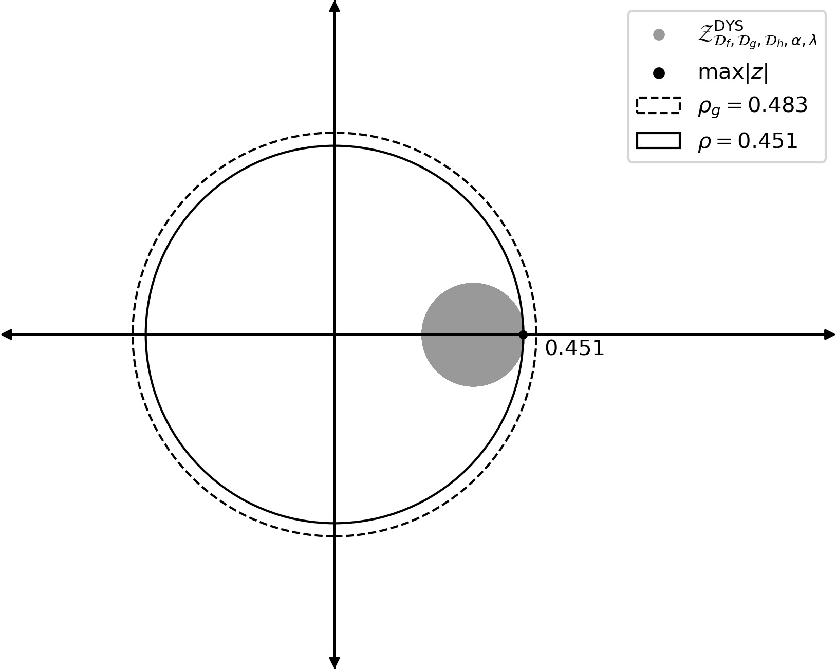
The explicit and simple description of 𝒵𝒜,ℬ,𝒞,α,λDYS{\mathcal{Z}}^{\text{DYS}}_{{\mathcal{A}},{\mathcal{B}},{\mathcal{C}},\alpha,\lambda} allows one to investigate it in a numerical and computer-assisted manner. Sampling points from 𝒵𝒟f,𝒟g,𝒟h,α,λDYS{\mathcal{Z}}^{\text{DYS}}_{{\mathcal{D}}_{f},{\mathcal{D}}_{g},{\mathcal{D}}_{h},\alpha,\lambda} is straightforward, and doing so provides a numerical estimate of the maximum modulus. For example, Figure 4 depicts 𝒵𝒟f,𝒟g,𝒟h,α,λDYS{\mathcal{Z}}^{\text{DYS}}_{{\mathcal{D}}_{f},{\mathcal{D}}_{g},{\mathcal{D}}_{h},\alpha,\lambda} with a specific choice of μf\mu_{f}, μg\mu_{g}, μh\mu_{h}, LfL_{f}, LgL_{g}, LhL_{h}, α\alpha, and λ\lambda. It shows that ρg\rho_{g}, the contraction factor of Theorem 1, is valid but not tight; the gap between 𝒵𝒟f,𝒟g,𝒟h,α,λDYS{\mathcal{Z}}^{\text{DYS}}_{{\mathcal{D}}_{f},{\mathcal{D}}_{g},{\mathcal{D}}_{h},\alpha,\lambda} and Circ⁡(0,ρg){\mathrm{Circ}}(0,\rho_{g}) indicates the contraction factor has room for improvement. Interestingly, if we modify the proof of Theorem 1 to choose rr in (3) more carefully, we seem to obtain a tight contraction factor in the instance of Figure 4. Specifically, when we numerically minimize ρ\rho as a function of rr, we observe that Circ⁡(0,ρ){\mathrm{Circ}}(0,\rho) touches 𝒵𝒟f,𝒟g,𝒟h,α,λDYS{\mathcal{Z}}^{\text{DYS}}_{{\mathcal{D}}_{f},{\mathcal{D}}_{g},{\mathcal{D}}_{h},\alpha,\lambda} in Figure 4 and the contact indicates tightness.
Refer to caption
Figure 4: 𝒵𝒟f,𝒟g,𝒟h,α,λDYS{\mathcal{Z}}^{\text{DYS}}_{{\mathcal{D}}_{f},{\mathcal{D}}_{g},{\mathcal{D}}_{h},\alpha,\lambda} with Circ⁡(0,ρf){\mathrm{Circ}}(0,\rho_{f}), Circ⁡(0,ρg){\mathrm{Circ}}(0,\rho_{g}), and Circ⁡(0,ρ){\mathrm{Circ}}(0,\rho), where μf=0.7\mu_{f}=0.7, μg=2\mu_{g}=2, μh=0.8\mu_{h}=0.8, Lf=1.5L_{f}=1.5, Lg=3L_{g}=3, Lh=1.3L_{h}=1.3, α=0.9\alpha=0.9, and λ=1\lambda=1.

Acknowledgments

This work was supported by the Samsung Science and Technology Foundation (Project Number SSTF-BA2101-02).

References

  • [1] D. Davis, W. Yin, A three-operator splitting scheme and its optimization applications, Set-valued and variational analysis 25 (4) (2017) 829–858.
  • [2] M. Yan, A new primal–dual algorithm for minimizing the sum of three functions with a linear operator, Journal of Scientific Computing 76 (3) (2018) 1698–1717.
  • [3] Y. Wang, H. Zhou, S. Zu, W. Mao, Y. Chen, Three-operator proximal splitting scheme for 3-d seismic data reconstruction, IEEE Geoscience and Remote Sensing Letters 14 (10) (2017) 1830–1834.
  • [4] J. A. Carrillo, K. Craig, L. Wang, C. Wei, Primal dual methods for wasserstein gradient flows, Foundations of Computational Mathematics 22 (2) (2022) 389–443.
  • [5] D. Van Hieu, L. Van Vy, P. K. Quy, Three-operator splitting algorithm for a class of variational inclusion problems, Bulletin of the Iranian Mathematical Society 46 (4) (2020) 1055–1071.
  • [6] M. Weylandt, Splitting methods for convex bi-clustering and co-clustering, IEEE Data Science Workshop (2019).
  • [7] H. Heaton, D. McKenzie, Q. Li, S. W. Fung, S. Osher, W. Yin, Learn to predict equilibria via fixed point networks, arXiv preprint arXiv:2106.00906 (2021).
  • [8] F. J. Aragón-Artacho, D. Torregrosa-Belén, A direct proof of convergence of Davis–Yin splitting algorithm allowing larger stepsizes, Set-Valued and Variational Analysis 30 (2022) 1–19.
  • [9] M. N. Dao, H. M. Phan, An adaptive splitting algorithm for the sum of two generalized monotone operators and one cocoercive operator, Fixed Point Theory and Algorithms for Sciences and Engineering 2021 (1) (2021) 16.
  • [10] F. Pedregosa, On the convergence rate of the three operator splitting scheme, arXiv preprint arXiv:1610.07830 (2016).
  • [11] E. K. Ryu, A. B. Taylor, C. Bergeling, P. Giselsson, Operator splitting performance estimation: Tight contraction factors and optimal parameter selection, SIAM Journal on Optimization 30 (3) (2020) 2251–2271.
  • [12] H. Wang, M. Fazlyab, S. Chen, V. M. Preciado, Robust convergence analysis of three-operator splitting, Allerton Conference on Communication, Control, and Computing (2019).
  • [13] L. Condat, P. Richtárik, Randprox: Primal-dual optimization algorithms with randomized proximal updates, OPT 2022: Optimization for Machine Learning (Workshop in Neural Information Processing Systems) (2022).
  • [14] J. Lee, S. Yi, E. K. Ryu, Convergence analyses of davis–yin splitting via scaled relative graphs, SIAM Journal on Optimization 35 (1) (2025) 270–301.
  • [15] E. K. Ryu, R. Hannah, W. Yin, Scaled relative graphs: Nonexpansive operators via 2D Euclidean geometry, Mathematical Programming 194 (1–2) (2022) 569–619.
  • [16] H. H. Bauschke, P. L. Combettes, Convex Analysis and Monotone Operator Theory in Hilbert Spaces, 2nd Edition, Springer, 2017.
  • [17] E. K. Ryu, S. Boyd, Primer on monotone operator methods, Applied and Computational Mathematics 15 (1) (2016) 3–43.
  • [18] E. K. Ryu, W. Yin, Large-Scale Convex Optimization: Algorithms & Analyses via Monotone Operators, 1st Edition, Cambridge University Press, 2022.
  • [19] R. E. Bruck, On the weak convergence of an ergodic iteration for the solution of variational inequalities for monotone operators in Hilbert space, Journal of Mathematical Analysis and Applications 61 (1) (1977) 159–164.
  • [20] G. B. Passty, Ergodic convergence to a zero of the sum of monotone operators in Hilbert space, Journal of Mathematical Analysis and Applications 72 (2) (1979) 383–390.
  • [21] D. W. Peaceman, H. H. Rachford, Jr, The numerical solution of parabolic and elliptic differential equations, Journal of the Society for Industrial and Applied Mathematics 3 (1) (1955) 28–41.
  • [22] J. Douglas, H. H. Rachford, On the numerical solution of heat conduction problems in two and three space variables, Transactions of the American Mathematical Society 82 (2) (1956) 421–439.
  • [23] P.-L. Lions, B. Mercier, Splitting algorithms for the sum of two nonlinear operators, SIAM Journal on Numerical Analysis 16 (6) (1979) 964–979.
  • [24] D. Gabay, B. Mercier, A dual algorithm for the solution of nonlinear variational problems via finite element approximation, Computers & Mathematics with Applications 2 (1) (1976) 17–40.
  • [25] A. Yurtsever, A. Gu, S. Sra, Three operator splitting with subgradients, stochastic gradients, and adaptive learning rates, Neural Information Processing Systems (2021).
  • [26] A. Yurtsever, B. C. Vũ, V. Cevher, Stochastic three-composite convex minimization, Neural Information Processing Systems (2016).
  • [27] V. Cevher, B. C. Vũ, A. Yurtsever, Stochastic forward Douglas–Rachford splitting method for monotone inclusions, in: A. R. Pontus Giselsson (Ed.), Large-Scale and Distributed Optimization, 1st Edition, Springer, 2018, pp. 149–179.
  • [28] A. Yurtsever, V. Mangalick, S. Sra, Three operator splitting with a nonconvex loss function, International Conference on Machine Learning (2021).
  • [29] F. Pedregosa, K. Fatras, M. Casotto, Proximal splitting meets variance reduction, International Conference on Artificial Intelligence and Statistics (2019).
  • [30] C. Zong, Y. Tang, Y. J. Cho, Convergence analysis of an inexact three-operator splitting algorithm, Symmetry 10 (11) (2018) 563.
  • [31] F. Pedregosa, G. Gidel, Adaptive three operator splitting, International Conference on Machine Learning (2018).
  • [32] F. Cui, Y. Tang, Y. Yang, An inertial three-operator splitting algorithm with applications to image inpainting, Applied Set-Valued Analysis and Optimization 1 (2019) 113–134.
  • [33] A. Salim, L. Condat, K. Mishchenko, P. Richtárik, Dualize, split, randomize: Toward fast nonsmooth optimization algorithms, Journal of Optimization Theory and Applications (2022).
  • [34] X. Huang, E. K. Ryu, W. Yin, Scaled relative graph of normal matrices, Journal of Convex Analysis (2026).
  • [35] R. Pates, The Scaled Relative Graph of a Linear Operator, arXiv preprint arXiv:2106.05650 (2021).
  • [36] N. Ogura, I. Yamada, Non-strictly convex minimization over the fixed point set of an asymptotically shrinking nonexpansive mapping, Numerical Functional Analysis and Optimization 23 (1-2) (2002) 113–137.
  • [37] T. Chaffey, F. Forni, R. Sepulchre, Graphical nonlinear system analysis, IEEE Transactions on Automatic Control 68 (10) (2023) 6067–6081.
  • [38] T. Chaffey, F. Forni, R. Sepulchre, Scaled relative graphs for system analysis, IEEE Conference on Decision and Control (2021).
  • [39] T. Chaffey, R. Sepulchre, Monotone One-Port Circuits, IEEE Transactions on Automatic Control 69 (2) (2024) 783–796.
  • [40] T. Chaffey, A rolled-off passivity theorem, Systems & Control Letters 162 (2022) 105–198.
  • [41] T. Chaffey, A. Padoan, Circuit model reduction with scaled relative graphs, IEEE Conference on Decision and Control (2022).
  • [42] Y. Nesterov, Introductory Lectures on Convex Optimization: A Basic Course (2014).
  • [43] K. Guo, On the linear convergence rate of a relaxed forward-backward splitting method, Optimization 70 (5-6) (2021) 1161–1170.