Quantum algorithms for optimal effective theory of many-body systems

We evaluate the loss function $F(x)=\left|\bra{\tilde{\psi}}\tilde{U}(x)\ket{\tilde{\psi}}\right|$ according to the amplitude amplification and estimation algorithm bib:34. As shown in Fig. 1(c), this is realized using the quantum phase estimation algorithm bib:14 within Grover’s search routine. The elementary transformation in amplitude amplification is formed of two phase-flip operators conditioned on the state, which reads

Here, $\tilde{U}(x)$ is the composite evolution operator corresponding to the effective Hamiltonian $H_{eff}(x)$. Given the initial state $\ket{\tilde{\psi}}$, $R_{x}$ is equivalent to a rotation in the subspace spanned by $\left\{\ket{\tilde{\psi}},\tilde{U}(x)\ket{\tilde{\psi}}\right\}$. The rotation is expressed as $R_{x}=e^{i\sigma_{y}\theta_{x}}$, where $\sigma_{y}$ is a Pauli operator, and we can find $\cos\frac{\theta_{x}}{2}=F(x)=\left|\bra{\tilde{\psi}}\tilde{U}(x)\ket{\tilde{\psi}}\right|$ is the loss function. The Pauli operator acts on the two-dimensional subspace, whose eigenstates are $\ket{y\pm}$ corresponding to eigenvalues $\pm 1$, respectively. The relation between eigenstates and $\left\{\ket{\tilde{\psi}},\tilde{U}(x)\ket{\tilde{\psi}}\right\}$ is given by

and

The loss function is evaluated by reading phases $e^{\pm i\theta_{x}}$ using the quantum phase estimation algorithm. To implement the algorithm, we need to introduce a register in addition to the register of $\ket{\tilde{\psi}}$, which is initialized in the state $\ket{\varphi}=\frac{1}{\sqrt{K}}\sum_{k=0}^{K-1}\ket{k}$. Here, the integer $K$ determines the resolution of the loss function evaluation. The quantum phase estimation is accomplished with the transformation

where $U_{QFT}$ denotes the quantum Fourier transformation bib:14. The quantum circuit for $R_{x}^{k}$ is shown in Fig. 7 of Appendix A, and the detailed process is summarized below:

$\ket{A_{+}}$ and $\ket{A_{-}}$ are given by

where $\theta=\frac{2\pi m}{K}$, $m=-\frac{K}{2}+1,\ldots,-1,0,1,\ldots,\frac{K}{2}$ assuming $K$ is even, $\ket{-\pi}\equiv\ket{\pi}$ and $f_{\theta}=\frac{1}{K}\sum_{k}e^{i(\theta_{x}-\theta)k}$. The distribution $|f_{\theta}|$ is concentrated at $\theta_{x}$ with the width $\sim\frac{2\pi}{K}$. If $\theta_{x}$ is in $\{\theta\}$, $\ket{A_{\pm}}=\ket{\pm\theta_{x}}$. Therefore, the information of the loss function has been stored in the register $\ket{\theta}$, and we can extract the information by measuring the value of $\theta$. Note that to carry out the accelerated search, here $\ket{A_{\pm}}$ will not be directly measured.

We now introduce the method to amplify amplitudes for $F(x)>\cos\frac{\theta_{th}}{2}$. To do so, we need to realize a phase flip depending on the loss function, i.e., $\theta$. However, because the loss function estimation has a finite resolution, the phase flip is inexact. We approximate the loss function-dependent phase flip with the operator

where $\Pi_{ini}=|\varphi\rangle\langle\varphi|\otimes|\tilde{\psi}\rangle\langle\tilde{\psi}|$, $U_{th}=\openone-2\sum_{-\theta_{th}<\theta<\theta_{th}}|\theta\rangle\langle\theta|$ is the phase flip depending on $\theta$.

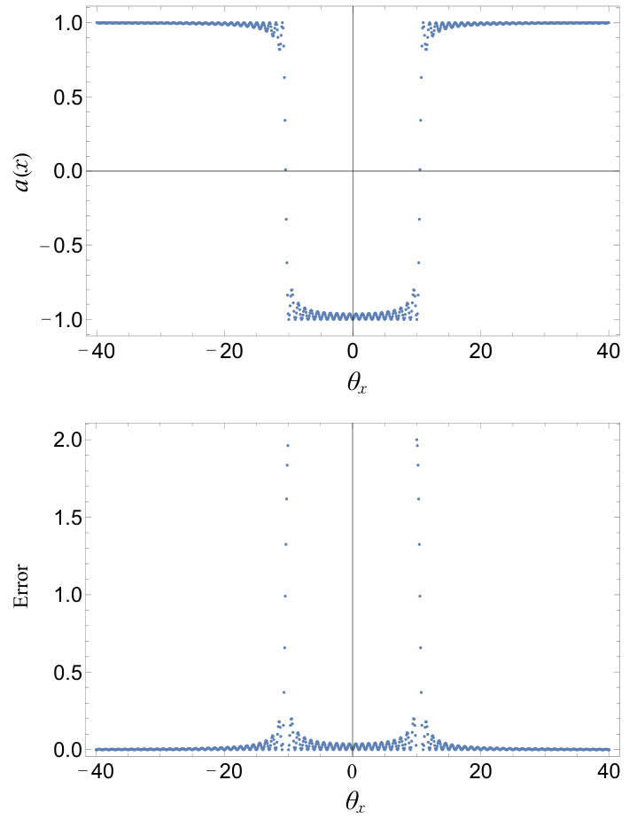
Because the distribution of $\theta$ is concentrated at $\theta_{x}$, the $\theta$-dependent phase flip results in a $\theta_{x}$-dependent phase. Firstly, let’s suppose $\theta_{x}\in\{\theta\}$: If $|\theta_{x}|<\theta_{th}$, we have $U_{th}\ket{A_{\pm}}=-\ket{A_{\pm}}$; If $|\theta_{x}|\geq\theta_{th}$, we have $U_{th}\ket{A_{\pm}}=\ket{A_{\pm}}$. In general $\theta_{th}$ is not one of $\theta$ values because of the finite resolution, and in this case, the effect of $U_{th}$ is not a simple phase change. We note that this problem caused by the finite resolution is only severe when $\theta_{x}$ is close to $\pm\theta_{th}$. When $\theta_{x}$ is significantly far away from the threshold $\pm\theta_{th}$, the distribution is concentrated on one side of the threshold, and we can neglect the probability on the other side.

We can detect the problem caused by the finite resolution by measuring the finial state after an inverse quantum phase estimation operator. If $\theta_{x}\in\{\theta\}$, a phase is applied on the state by $U_{th}$, and the inverse quantum phase estimation transforms the state back to the initial state $\ket{\varphi}\otimes\ket{\tilde{\psi}}$ up to a $\theta_{x}$-dependent phase. If $\theta_{x}\notin\{\theta\}$, the state does not go back to the exact initial state. If the measurement outcome is not $\ket{\varphi}\otimes\ket{\tilde{\psi}}$, we know that the $\theta_{x}$-dependent phase flip has failed. If the outcome is $\ket{\varphi}\otimes\ket{\tilde{\psi}}$, we obtain the finial state

where

is always real and in the interval $[-1,1]$. If $\theta_{x}\in\{\theta\}$, $a_{x}=\pm 1$ depending on $\theta_{x}$. If $\theta_{x}\notin\{\theta\}$ and $\theta_{x}$ is significantly far away from $\pm\theta_{th}$, we still have $a_{x}\approx\pm 1$. To illustrate this, we set $K=4096$ and $|\theta_{th}|=10*\frac{2\pi}{K}$, and plot $a(x)$ with a change of $\theta_{x}$ in Fig. 2. We see that the error is significant only when $\theta_{x}$ is close to $|\theta_{th}|$. With this approximate $\theta_{x}$-dependent phase flip, we can realize the accelerated search.

We use Grover’s algorithm to find effective Hamiltonian operators with a loss function that exceeds the threshold. Accordingly, we need a register to store the parameter $x$, which is initialized in the state $\ket{X}=\frac{1}{\sqrt{N}}\sum_{x}\ket{x}$. Amplitudes of states with $|\theta_{x}|<\theta_{th}$ are amplified by iterating two operators $V_{X}=(\openone-2|X\rangle\langle X|)\otimes\openone\otimes\openone$ and $V_{th}^{ideal}$ on the initial state of the total system $\ket{X}\otimes\ket{\varphi}\otimes\ket{\tilde{\psi}}$. Here,

where $\eta_{x}=-1$ if $|\theta_{x}|<\theta_{th}$ and $\eta_{x}=1$ if $|\theta_{x}|\geq\theta_{th}$. If the number of effective Hamiltonian operators satisfying $|\theta_{x}|<\theta_{th}$ is $M$, we can find one of them in $O(\sqrt{N/M})$ iterations bib:14.

In our algorithm, we approximate $V_{th}^{ideal}$ with a controlled $V_{th}(x)$, and the operator on the total system is

Because $|a_{x}|$ is smaller than one in the vicinity of the threshold $\pm\theta_{th}$, it leads to probability leakage: For each iteration, there is a finite probability that the $\theta_{x}$-dependent phase flip fails, i.e., the measurement outcome is not $\ket{\varphi}\otimes\ket{\tilde{\psi}}$. Next, we analyze the impact of this probability leakage.

The error due to the difference between $V_{th}$ and $V_{th}^{ideal}$ after $j$ iterations is

Here, we have neglected $\ket{\varphi}\otimes\ket{\tilde{\psi}}$ for simplicity, we have used that $\|V_{X}\|=1$ and $\|V_{th}\|\leq 1$ for the matrix 2-norm. Then, the error has the upper bound

where

Suppose

we have

Note that one can work out the expression of $\alpha_{x}$ straight-forwardly following Grover’s algorithm bib:14. The error $|\eta_{x}-a_{x}|$ is non-zero only in the vicinity of the threshold $\pm\theta_{th}$ with a radius $\sim\frac{2\pi}{K}$, see Fig. 2. Therefore, to implement the accelerated effective-Hamiltonian search, we need to choose a sufficiently large $K$ such that the radius is small, and there is no effective Hamiltonian within the radius.

In this section, we introduce the implementation details of the operator $\tilde{U}(x)$ which formed the operator $R_{x}$ in Eq. 9. Here, we can define the time-evolution operators as

$x$ is the label of an effective Hamiltonian, and $t$ is evolution time. According to Eq. 7, the operator $\tilde{U}(x)$ is a composite evolution operator

For the total system, the operator $U(x,t_{i})$ is

with different evolution times $t_{i}$. The following outlines the method for implementing $U_{X}(t_{i})$. Without loss of generality, the candidate effective Hamiltonian can be represented as

Here, the variable $x$ can be expressed as a vector $x=(\lambda_{1},\lambda_{2},...,\lambda_{m})$. $H_{i}$ represents all possible terms that may appear in the effective Hamiltonian, while $\lambda_{i}$ denotes their coefficients, which need to be determined by our algorithm, and $m$ is the number of terms. To implement the operator $U_{X}(t_{i})$ , we substitute Eq. 29 into Eq. 28 and have

Here, $n_{t}$ denotes the Trotter steps, and $n$ represents the number of qubits used to encode one coefficient $\lambda_{i}$. $\epsilon$ is a small constant that signifies the resolution of the coefficients: The second equality in Eq. 30 is based on the Trotter-Suzuki decomposition, and

where $i_{m,n}=0,1$. For simplicity, we assume that the signs of all terms $\lambda_{i}H_{i}$ are contained within $H_{i}$, and the values of all $\lambda_{i}$ are positive. It is important to note that we can find some coefficients to be equal to zero in the end, and this indicates that the corresponding terms should not be present in the correct effective Hamiltonian.

In our approach, the number of qubits and quantum gates required for implementing $U_{X}(t_{i})$ increases polynomially with $O(logN)$, where $N$ denotes the number of candidate effective Hamiltonian. As a result, when $N$ increases, our algorithm maintains its ability to achieve quadratic acceleration in the search process, while necessitating additional quantum resources that increase linearly. Note that, the method to implement $U_{X}(t_{i})$ is not unique, and our method described above is relatively universal. The quantum circuit to implement $U_{X}(t_{i})$ can be found in Fig. 6 of Appendix A.

To demonstrate the quadratic speedup of our algorithm in searching for the effective Hamiltonian, we present a numerical example in this section. We take the transverse-field Ising model bib:44 as an example to find its effective Hamiltonian. The Hamiltonian of the whole system is

Here, $\sigma^{z}_{i}$ and $\sigma^{x}_{i}$ are Pauli operators acting on the $i$-th site. $N$ denotes the number of spins. $\Delta$ and $J$ are coefficients. For this system, we can obtain the exact second-order efficient Hamiltonian on a low-energy subspace with the Schrieffer-Wolff (SW) method bib:45; bib:46; bib:47; bib:48; bib:49; bib:50; bib:51:

where $\lambda$ and $\kappa$ satisfy $\lambda=J$ and $\kappa=\frac{J^{2}}{2\varDelta}$. Here, the form of the projector is $P=\sum\limits_{i=1}^{N}\ket{\phi_{i}}\bra{\phi_{i}}$, where the vector $\ket{\phi_{i}}$ denote the n-th single-particle excited state and we can encode the state as $\ket{\phi_{1}}=\ket{00..001}$ and $\ket{\phi_{2}}=\ket{00..010}$ and so forth. The form of transformation $T$ is complex and determined by the Schrieffer-Wolff (SW) method. We performed numerical simulations using Grover’s algorithm to search for the effective Hamiltonian of a transverse-field Ising model. The process is simulated using Questlink bib:52; bib:53 on a classical computer.

The results are shown in Fig. 3. In our simulations, we set $N=2$, $\Delta=10$, and $J=1$. $\epsilon$ is set to be $1/7$. Therefore, the coefficient should satisfy $\lambda=J=7\epsilon$. The evolution time is $t=\pi$, and the Trotter steps is taken to be 1000. We use 10 qubits to implement our algorithm, of which 4 qubits are for encoding the coefficients $x$, 4 qubits are for implementing the quantum Fourier transform in Eq. 12, and 2 qubits are used for simulating the transverse-field Ising model. We numerically display the probability distribution of the computational basis $\ket{x}$ when applying the Grover iteration for 0, 1, 3, and 4 times, respectively. For a classical algorithm, it requires $2^{4}$ unstructured searching operations to search for the correct coefficients. However, our algorithm needs only $\sqrt{2^{4}}$ Grover oracle operations to find the target state with high probability, as shown in Fig. 3.

The variational quantum simulation bib:36; bib:37; bib:38; bib:39; bib:40; bib:41; bib:42 is a hybrid classical-quantum algorithm that has various applications in solving many-body problems. With a quantum computer, we first have a trial state $\ket{\Psi(\vec{\theta})}$ that can be prepared by a quantum circuit with a parameterized gate set. The state at time $t$ is represented as $\ket{\Psi(t)}=\ket{\Psi(\vec{\theta}(t))}$ with time-dependent parameters $\vec{\theta}(t)$. The variational quantum simulation is used to find the best solution $\vec{\theta}(t+\delta t)$ such that the state evolves from $\ket{\Psi(\vec{\theta}(t))}$ to $\ket{\Psi(\vec{\theta}(t+\delta t))}$ according to Schrödinger’s equation:

Here, the test Hamiltonian $H_{test}$ is defined by $H-H_{eff}$. $H$, and $H_{eff}$ denotes the original Hamiltonian and the effective Hamiltonian respectively. To optimize the parameters, we take the method introduced in bib:43. The evolution of parameters can be found by solving

where the matrix elements of $A$ and $C$ are defined by

Then, we can iteratively update the parameters under

The overall flow of the variational quantum simulation is summarized as follows: First, we select initial parameters $\vec{\theta}(0)$ and a small time step $\delta t$. Second, we solve Eq. 35 using the classical computer, in which the matrix $A_{i,j}$ and the vector $C_{i}$ in the equation are evaluated using the quantum computer. Repeating the second step, we can get the solution that approximates Eq. 34.

We take the transverse-field Ising model showing in Eq. 32 as an example. To find the optimal effective Hamiltonian in a set of candidates, we choose $N_{t}$ trials $(\ket{\psi_{i}(\vec{\theta}(0))},t)$ with initial states $\ket{\psi_{i}(\vec{\theta}(0))}$ and evolution time $t$ to maximize the average fidelity

corresponding to Eq. 3, where the parameter $\vec{\theta}(t)$ is determined by Eq. 37 with a fixed time step $\delta_{t}=2\pi/1000$. The trial state at time $t$ is given by

We evaluate the average fidelity corresponding to Eq. 38 with different coefficients of the test Hamiltonian $H_{test}$. When given an initial coefficient $x_{0}=(\lambda_{0},\kappa_{0})$, we can use the gradient ascent method bib:54.1 to maximize the loss function defined in Eq. 38. In our example, there are only two parameters that need to be determined. Therefore, we employed the grid search method to identify the optimal parameters.

We performed numerical simulations using Questlink on a classical computer and experiments on IBM’s cloud quantum computer ”ibmq-athens”. We take $N=5$, $\Delta=10$ and $J=1$. Then the exact values of the coefficients in the effective Hamiltonian $H_{eff}$ are $\lambda=J=1$ and $\kappa=\frac{J^{2}}{2\varDelta}=0.05$. We choose $\sigma^{x}_{i}\ket{00000}$ $(i=1,..,5)$ as the initial states, where $\sigma^{x}_{i}$ is the Pauli operator acting on the $i$-th site. The ansatz is chosen as the 3-step trotter circuit.

The results are shown in Fig. 4. In both simulations and experiments, we see that when $\lambda$ and $\kappa$ are close to the exact values, the average fidelity $F_{ave}$ becomes higher. Owing to circuit noise, measurement error and shot noise (shots = 8192), the resolution of the coefficients to be determined with experimental results is about 0.01$\sim$0.02 and the fidelity obtained from experiments is generally lower than that from simulations. Nevertheless, in both cases, the fidelity reaches the maximum at the correct value of the coefficients $\lambda=1$ and $\kappa=0.05$.

Note that the state in Eq. 39 can also be realized with the Trotter-Suzuki decomposition bib:22 at the cost of deeper quantum circuits. According to the method, the time evolution operator $U(t)$ becomes

where $H_{test}=H-H_{eff}$ is expressed as $H_{test}=\sum_{j}H_{j}$ and $t$ denotes the total time of evolution. Each term $e^{-iH_{j}\tau}$ represents the evolution driven by $H_{j}$ for a short time $\tau$, which can be realized with quantum gates. Usually, $\tau=t/n_{t}$, and when $n_{t}$ is larger, the approximation is better. In our simulations we fix $\tau=2\pi/1000$.

Fig. 5 shows the evolution of the average fidelity of the quantum states obtained from the Trotter and the variational method simulated classically. We see that the two methods show very similar performance since the two curves nearly overlap as $t$ changes. However, the trotter method uses much deeper circuits, e.g., with over $10^{3}$ more gates than those required in the variational method at $t=6\pi$. Therefore, our method is more suitable for NISQ devices.

References

- (1) E. Epelbaum, H.-W. Hammer and U.-G. Meissner, Modern theory of nuclear forces, Rev. Mod. Phys. 81, 1773 (2009).
- (2) R. Machleidt and D. R. Entem, Chiral effective field theory and nuclear forces, Phys. Rept. 503, 1 (2011).
- (3) Bing-Nan Lu, Ning Li, Serdar Elhatisari, Dean Lee, Evgeny Epelbau, Ulf-G. meissner, Essential elements for nuclear binding, Phys. Lett. B 797, 134863 (2019).
- (4) M. Piarulli, A. Baroni, L. Girlanda, A. Kievsky, A. Lovato, E. Lusk, L. E. Marcucci, S. C. Pieper, R. Schiavilla, M. Viviani and R. B. Wiringa, Light-Nuclei Spectra from Chiral Dynamics, Phys. Rev. Lett. 120, 052503 (2018).
- (5) B. S. Hu, W. G. Jiang, T. Miyagi, Z. H. Sun, A. Ekstrom, C. Forssen, G. Hagen, J. D. Holt, T. Papenbrock, S. R. Stroberg and I. Vernon, Ab initio predictions link the neutron skin of 208Pb to nuclear forces, Nat. Phys. 18, 1196 (2022).
- (6) M. Leonhardt, M. Pospiech, B. Schallmo, J. Braun, C. Drischler, K. Hebeler, A. Schwenk, Symmetric nuclar matter from the strong interaction, Phys. Rev. Lett. 125, 142502 (2020).
- (7) Bing-Nan Lu, Ning Li, Serdar Elhatisari, Dean Lee, Joaquín E. Drut, Timo A. Lähde, Evgeny Epelbaum, and Ulf-G. Meißner, Ab initio nuclar thermodynamics, Phys. Rev. Lett. 125, 192502 (2020).
- (8) Serdar Elhastisari, Dean Lee, Gautam Rupak, Evgeny Epelbaum, Hermann Krebs, Timo A. Lahde, Thomas Luu and Ulf-G. Meissner, Ab initio alpha-alpha scattering, Nature 528, 111 (2015).
- (9) V. Durant, P. Capel, L. Huth, A. B. Balantekin and A. Schwenk, Double-folding potentials from chiral effective field theory, Phys. Lett. B 782, 668 (2018).
- (10) Kenneth G. Wilson, The renormalization group: Critical phenomena and the Kondo problem, Rev. Mod. Phys. 47, 773 (1975).
- (11) M. C. Birse, J. A. McGovern, K. G. Richardson, A renormalization-group treatment of two-body scattering, Phys. Lett. B 464, 169 (1999).
- (12) R. Peierls, On Ising’s model of ferromagnetism. Mathematical Proceedings of the Cambridge Philosophical Society 32, 477 (1936)
- (13) Shor, Peter W. ”Algorithms for quantum computation: discrete logarithms and factoring.” Proceedings 35th annual symposium on foundations of computer science. Ieee, 1994.
- (14) M. A. Nielsen and I. L. Chuang, “Quantum Computation and Quantum Information,” Cambridge University Press, Cambridge (2000).
- (15) I. M. Georgescu, S. Ashhab, and Franco Nori, Quantum simulation. Rev. Mod. Phys. 86, 153 (2014)
- (16) David Poulin, Angie Qarry, Rolando Somma, and Frank Verstraete, Quantum simulation of time-dependent hamiltonians and the convenient illusion of hilbert space. Phys. Rev. Lett. 106, 170501 (2011)
- (17) E. F. Dumitrescu, A. J. McCaskey, G. Hagen, G. R. Jansen, T. D. Morris, T. Papenbrock, R. C. Pooser, D. J. Dean, and P. Lougovski, Cloud Quantum Computing of an Atomic Nucleus. Phys. Rev. Lett 120, 210501 (2018)
- (18) S Mcardle, S Endo, A Aspuru-Guzik, S Benjamin, X Yuan, Quantum computational chemistry. Rev. Mod. Phys. 92, 015003 (2020)
- (19) Yudong Cao, et al, Quantum chemistry in the age of quantum computing. Chemical Reviews 08, (2019)
- (20) S. Kais, K.B. Whaley, A.R. Dinner, and S.A. Rice, Quantum Information and Computation for Chemistry. Advances in Chemical Physics, Wiley, (2014)
- (21) Kitaev, A. Yu, Quantum measurements and the Abelian stabilizer problem. arXiv preprint quant-ph/9511026 (1995).
- (22) H. F. Trotter, On the Product of Semi-groups of Operators,Proc. Am. Math. Soc. 10, 545 (1959).
- (23) Frank Arute1, et al, Quantum supremacy using a programmable superconducting processor. Nature, 574: 505-510 (2019).
- (24) Alberto Peruzzo, A variational eigenvalue solver on a photonic quantum processor. Nat. Commun. 5, 4213 (2014)
- (25) Kandala A, Mezzacapo A, Temme K, et al. Hardware-efficient variational quantum eigensolver for small molecules and quantum magnets. Nature, 549(7671): 242-246(2017).
- (26) Google AI Quantum. ”Hartree-Fock on a superconducting qubit quantum computer.” Science 369.6507 (2020): 1084-1089.
- (27) Carlos E. Solivérez, General theory of effective Hamiltonians. Phys. Rev. A. 24, 4 (1981)
- (28) Bogner S K, Kuo T T S, Schwenk A, Model-independent low momentum nucleon interaction from phase shift equivalence. Physics Reports 386, 1-27 (2003)
- (29) Sergey Bravyi, David P. DiVincenzo, Daniel Loss, Schrieffer–Wolff transformation for quantum many-body systems. Annals of Physics. 326, 2793-2826 (2011)
- (30) F. C. Zhang and T. M. Rice, Effective Hamiltonian for the superconducting Cu oxides. Phys. Rev. B 37, 3759 (1988)
- (31) C. D. Batista and A. A. Aligia, Effective Hamiltonian for cuprate superconductors. Phys. Rev. B 47, 8929 (1993)
- (32) K. Tsukiyama, S. K. Bogner, A. Schwenk, In-medium Similarity Renormalization Group for Nuclei. Phys. Rev. Lett. 106, 222502 (2011)
- (33) S. R. White, Numerical canonical transformation approach to quantum many-body problems. J. Chem. Phys. 117, 7472 (2002)
- (34) G Brassard, P Hoyer, M Mosca, A Tapp, Quantum Amplitude Amplification and Estimation. Quantum computation and information 305, 53-74 (2002).
- (35) S. Sachdev, Quantum Phase Transitions. Cambridge University Press, Cambridge (2011).
- (36) JR Schrieffer, PA Wolff, Relation between the Anderson and Kondo Hamiltonians. Phys. Rev. 149, 2 (1966)
- (37) M. M. Salomaa, Schrieffer-Wolff transformation for the Anderson Hamiltonian in a superconductor. Phys. Rev. B 37, 9312 (1988)
- (38) E. M. Kessler, Generalized Schrieffer-Wolff formalism for dissipative systems. Phys. Rev. A 86, 012126 (2012)
- (39) Seung-Sup B. Lee, Jan von Delft, and Andreas Weichselbaum, Generalized Schrieffer-Wolff transformation of multiflavor Hubbard models. Phys. Rev. B 96, 245106 (2017)
- (40) Jonathan Wurtz, Pieter W. Claeys, and Anatoli Polkovnikov, Variational Schrieffer-Wolff transformations for quantum many-body dynamics. Phys. Rev. B 101, 014302 (2020)
- (41) Raymond Chan, The exact Schrieffer–Wolff transformation. Philosophical Magazine 84, 1265 (2004)
- (42) Marin Bukov, Michael Kolodrubetz, and Anatoli Polkovnikov, Schrieffer-Wolff Transformation for Periodically Driven Systems: Strongly Correlated Systems with Artificial Gauge Fields. Phys. Rev. Lett 116, 125301 (2016)
- (43) Tyson Jones, Simon Benjamin, QuESTlink Mathematica embiggened by a hardware-optimised quantum emulator. Quantum Science and Technology. 5, 513 (2020)
- (44) Tyson Jones, Anna Brown, Ian Bush and Simon C. Benjamin, QuEST and High Performance Simulation of Quantum Computers. Scientific Reports. 9, 10736 (2019)
- (45) John Preskill, Quantum Computing in the NISQ era and beyond. Quantum 2, 79 (2018)
- (46) Xiao Yuan, Suguru Endo, Qi Zhao, Ying Li, and Simon C. Benjamin, Theory of variational quantum simulation. Quantum. 3, 192 (2019).
- (47) Jutho Haegeman, J. Ignacio Cirac, Tobias J. Osborne, Iztok Pizorn, Henri Verschelde, and Frank Verstraete, Time-dependent variational principle for quantum lattices. Phys. Rev. Lett. 107, 070601 (2011).
- (48) J. Broeckhove, L. Lathouwers, E. Kesteloot, and P. Van Leuven, On the equivalence of time dependent variational principles. Chemical Physics Letters 149, 547-550 (1988).
- (49) Suguru Endo, Jinzhao Sun, Ying Li, Simon C. Benjamin, and Xiao Yuan, Variational Quantum Simulation of General Processes. Phys. Rev. Lett 125, 010501 (2020)
- (50) Sam McArdle, Tyson Jones, Suguru Endo, Ying Li, Simon C. Benjamin and Xiao Yuan, Variational ansatz-based quantum simulation of imaginary time evolution. npj Quantum Information volume 5, 75 (2019)
- (51) Tyson Jones, Suguru Endo, Sam McArdle, Xiao Yuan, and Simon C. Benjamin, Variational quantum algorithms for discovering Hamiltonian spectra. Phys. Rev. A 99, 062304 (2019)
- (52) Ming-Cheng Chen, Ming Gong, Xiaosi Xu, Xiao Yuan, Jian-Wen Wang, Can Wang, et al, Demonstration of Adiabatic Variational Quantum Computing with a Superconducting Quantum Coprocessor. Phys. Rev. Lett 125, 180501 (2020)
- (53) Ying Li and Simon C. Benjamin, Efficient Variational Quantum Simulator Incorporating Active Error Minimization,Phys. Rev. X. 7, 021050 (2017).
- (54) Ruder, Sebastian. ”An overview of gradient descent optimization algorithms.” arXiv preprint arXiv:1609.04747 (2016).
- (55) IBM Quantum, https://quantum-computing.ibm.com/ (2021).