Mathematical Programming Formulations for the Collapsed k-Core Problem00footnotetext: ©2023. This manuscript version is made available under the CC-BY-NC-ND 4.0 license https://creativecommons.org/licenses/by-nc-nd/4.0/. Accepted for publication in European Journal of Operational Research; doi: 10.1016/j.ejor.2023.04.038
Email addresses: cerulli@essec.edu (M. Cerulli), dserra@unisa.it (D. Serra), csorgente@unisa.it (C. Sorgente), archetti@essec.edu (C. Archetti), ivana.ljubic@essec.edu (I. Ljubić)
Abstract
In social network analysis, the size of the -core, i.e., the maximal induced subgraph of the network with minimum degree at least , is frequently adopted as a typical metric to evaluate the cohesiveness of a community. We address the Collapsed -Core Problem, which seeks to find a subset of users, namely the most critical users of the network, the removal of which results in the smallest possible -core. For the first time, both the problem of finding the -core of a network and the Collapsed -Core Problem are formulated using mathematical programming. On the one hand, we model the Collapsed -Core Problem as a natural deletion-round-indexed Integer Linear formulation. On the other hand, we provide two bilevel programs for the problem, which differ in the way in which the -core identification problem is formulated at the lower level. The first bilevel formulation is reformulated as a single-level sparse model, exploiting a Benders-like decomposition approach. To derive the second bilevel model, we provide a linear formulation for finding the -core and use it to state the lower-level problem. We then dualize the lower level and obtain a compact Mixed-Integer Nonlinear single-level problem reformulation. We additionally derive a combinatorial lower bound on the value of the optimal solution and describe some pre-processing procedures, and valid inequalities for the three formulations. The performance of the proposed formulations is compared on a set of benchmarking instances with the existing state-of-the-art solver for mixed-integer bilevel problems proposed in (Fischetti et al. 2017).
1 Introduction
In recent years, with the advent of social networks era, studying the behaviour of the users in a network has gained increasing interest. Particularly important are the so-called critical users, i.e., the ones who have a large number of connections with other users and whose departure from the network might potentially cause the exit of many other users. Indeed, a property of social networks is that the decision of each user (leaving or remaining in the network) is influenced by that of her connected friends. A popular assumption is that a user remains in the network if she has at least a certain number of connections, say , in the network (Bhawalkar et al. 2015). On the contrary, a user is driven to leave the social network if she has less than connections. Given this assumption, if a user leaves the network, the degree of her neighbors decreases by one, eventually becoming smaller than for some of them. Thus, a cascade phenomenon is observed each time a user drops out from the network, until a stable configuration is obtained, which corresponds to the -core of the social network graph.
In this context, we study the Collapsed -Core Problem, which has been introduced in (Zhang et al. 2017b) to identify the critical users to be eventually incentivized not to leave the network (or, from an adversarial point of view, to leave it). This problem indeed consists in finding the set of a given number of users, whose exit from the network minimizes the number of the remaining users in the network itself, i.e., leads to the minimal -core. First of all, we propose a formulation of the problem modeling the cascade effect which determines the withdrawal of a certain number of users from the network. In such approach, a time index is needed to represent the subsequent deletion rounds of this process. Beyond that, the tools of bilevel optimization have been recently used for developing exact methods for several critical node/edge detection problems (Furini et al. 2019; Furini et al. 2020; Furini et al. 2021; Furini et al. 2022). These works show that novel and computationally effective mathematical programming formulations can be derived thanks to the bilevel interpretation of the problems. Motivated by these studies, we use bilevel programming to model the Collapsed -Core Problem, discarding the time index. A bilevel program is an optimization problem where one problem is nested into another (Vicente and Calamai 1994; Colson et al. 2007; Dempe 2002; Cerulli 2021; Kleinert et al. 2021). The formulation of a classical bilevel problem reads
| s.t. | () | |||
The outer optimization problem in the variables and is the so-called upper-level problem. The inner optimization problem in the variable , parameterized with respect to the upper-level variables , is the so-called lower-level problem. In formulation (1), we implicitly assume that the lower-level problem has only one optimal solution for each value of . If this is not the case, this formulation is the one obtained with the so-called optimistic approach (Dempe 2002), which consists in selecting the lower-level optimal solution corresponding to the best outcome for the upper level that minimizes it. The whole bilevel problem can be seen as a hierarchical decision process: in the upper level, a leader makes a decision while anticipating the optimal reaction of the lower-level decision maker, the follower, whose decision depends on the decision of the leader. Another way to formulate problem is
| s.t. | |||
where is the so called value function of the lower level.
In the Collapsed -Core Problem, the hierarchical structure can be described as follows. We can see the follower as an entity who is computing the collapsed -core resulting after the decision of the leader on the nodes to interdict from the network. So, the follower aims at identifying the subgraph of maximum cardinality, resulting from the interdiction of the nodes selected by the leader, satisfying the property that each node of the subgraph has at least neighbors. The leader instead aims at detecting the set of nodes for which the cardinality of the associated subgraph is minimized, which corresponds to the set of the most critical users in the network.
Contributions
It is well-known that the problem of finding the -core of a graph, denoted as -Core Detection Problem in the following, can be solved in polynomial time (see Batagelj and Zaversnik 2002), and one can easily model the problem using binary variables. However, to the best of our knowledge, prior to the current work, no Integer Linear Programming (ILP) or Linear Programming (LP) formulation (and, thus, a polynomial approach based on LP) for the -Core Detection Problem was known. In this work we provide a first compact LP formulation for calculating the -core. In addition, as far as we know, no mathematical programming formulations for the Collapsed -Core Problem (Zhang et al. 2017b) have ever been investigated in the existing literature. We provide three integer programming formulations, and propose to enhance them with a combinatorial lower bound and valid inequalities. The first formulation is a compact time-expanded model that mimics the iterative node “collapsing” process. The two other models are based on the bilevel interpretation of the problem. The first is a sparse formulation that projects out the lower-level variables and exploits a Benders-like decomposition. The second exploits the LP-based formulation of the -Core Detection Problem, and the LP-duality. All the three formulations are implemented and computationally evaluated against the state-of-the-art bilevel solver from Fischetti et al. 2017. The obtained results demonstrate the efficiency of the proposed approaches, with the model using the LP-duality exhibiting the best performances, both in terms of computing times and gaps at the termination.
The rest of the paper is organized as follows. In Section 2, we review the main literature in the field. In Section 3 we introduce the needed definitions and notations. In Section 4, we present two mathematical programming formulations of the -Core Detection Problem. In Section 5, we introduce different mathematical programming formulations for the Collapsed -Core Problem: first a time-dependent model, then two bilevel programs, which mainly differ in the lower level, where the two formulations proposed in Section 4 are used. In Section 6, we describe pre-processing procedures, as well as valid inequalities that strengthen the proposed formulations. In Section 7, we describe how to separate the valid inequalities which are exponential in number. Section 8 is devoted to the numerical experiments, and Section 9 concludes the paper.
2 Literature Review
We consider the following definition of the -core:
Definition 1.
Given an undirected graph , and a positive integer , the -core of is the maximal induced subgraph of in which all the nodes have degree at least .
The -core may be calculated as the resulting graph obtained by iteratively deleting from all the nodes that have degree less than , in any order. This procedure is known as the -core decomposition (Sariyüce and Pinar 2016), the basic theory of which is surveyed in (Malliaros et al. 2020). We point out that the original definition of the -core given by Seidman 1983 requires the connectedness of the -core. In (Matula and Beck 1983), this original definition is used, and an algorithm, named Level Component Priority Search, is introduced for finding all the maximal connected components of a graph with degree at least . However, in most of the recent papers in the field, the connectedness requirement is relaxed, starting from Batagelj and Zaversnik 2002, where an algorithm with time complexity for core decomposition is proposed. This is why in Definition 1 we also assume that the -core may contain multiple connected components.
The Anchored -Core Problem is studied by Bhawalkar et al. 2015. It consists in anchoring nodes (nodes that remain engaged no matter what their friends do) to maximize the size of the corresponding anchored -core, i.e., the maximal subgraph in which every non-anchored node has degree at least . It may be useful to incentivize key individuals to stay engaged within the network, preventing the cascade effect. The Anchored -Core Problem is solvable in polynomial time for , but is -hard for (Bhawalkar et al. 2015). In (Zhang et al. 2017a) a greedy algorithm, called OLAK, is proposed to solve this problem, while in (Laishram et al. 2020) the so-called Residual Core Maximization heuristic is introduced. Another paper focusing on the maximization of the -core is (Chitnis et al. 2013), where improved hardness results on the Anchored -Core Problem are given.
From an antagonistic perspective, a natural question associated with the Anchored -Core Problem is how to maximally collapse the engagement of the network by incentivizing the most critical users to leave. This problem is called the Collapsed -Core Problem, and was introduced in (Zhang et al. 2017b). The aim is to find the set of nodes the deletion of which leads to the smallest -core (i.e., the -core with minimum cardinality), obtained from by iteratively removing nodes with degree strictly lower than . In (Zhang et al. 2017b), it is shown that the Collapsed -Core Problem is -hard for any and a greedy algorithm to compute feasible solutions for the problem is proposed. In (Luo et al. 2021), the parameterized complexity of the Collapsed -Core Problem is studied with respect to the parameters , , as well as another parameter, say , which represents the maximum allowed cardinality of the remaining -core (i.e., it should not have more than number of nodes). A further study on the -core minimization was conducted in (Zhu et al. 2018), where the focus was on edges instead of nodes. Indeed, the aim of the problem in this case is to identify a set of edges, so that the minimal -core is obtained by deleting these edges from the graph. This problem is proven to be -hard, and a baseline greedy algorithm is proposed.
In (Yu et al. 2019), the Collapsed -Core Problem is applied to determine the key scholars who should be engaged in various tasks in science and technology management, such as experts finding, collaborator recommendation, and so on. More recently, in (Zhang and Yang 2020), a related problem is studied: the Collapsed --community in signed graph. Given a signed graph, which is a graph where each edge has either a “” sign if representing a friendship or a “” sign if representing an enemy relationship, the --community is made of the users having not less than friends and no more than enemies in the community. This problem aims at finding the set of nodes the removal of which from the graph will lead to the minimum cardinality of the remaining --community.
3 Notations
Let us consider an undirected graph , with , and two positive integers and . Denote by the set of neighbors of node in graph i.e., the set . Furthermore, let be the minimum degree of the graph , which is the minimum of its nodes’ degrees. For a given set of nodes , let denote the subgraph of induced by , and thus its minimum degree. Moreover, let denote the subgraph of induced by , i.e., . Let be the -core of graph , i.e., the maximum cardinality subgraph in which every node has a degree at least . In the following, we will refer to the number of nodes in a given -core as its size or cardinality. Let us further define the -subcores of as the induced subgraphs of in which all the nodes have degree at least . From this definition, it is clear that the -core of coincides with its -subcore of largest cardinality and, while there may exist several -subcores, the -core of is always unique. Finally, we say that a node of has coreness (or core number) if it belongs to a -subcore, but not to any -subcore.

In Figure 1, a graph is shown and each node is colored according to its core number. In particular, the two orange nodes have coreness , meaning that they do not belong to any -subcore with ; the five green nodes, instead, have coreness two, since is the maximum value of such that there exist a -subcore including any of them; finally, the remaining seven cyan nodes have coreness , indeed they together form a -subcore.
A detailed list of the notations used in the paper can be found in A.
4 Mathematical formulations for the -Core Detection Problem
In this section we propose two formulations for the -Core Detection Problem. The first one is an ILP model defined in the space of binary variables associated with the set of nodes. The second one is a compact, extended formulation which models the subgraph induced by the set of nodes that are outside the -core. In this second model, which uses node and edge variables, the integrality constraints can be relaxed, and hence LP formulation can be obtained.
4.1 ILP Formulation
The binary variables involved in the first formulation are defined as:
| (1) |
Let
| (2) |
be the set of incident vectors of any subgraph in the nodes of which have degree at least (i.e., any -subcore of ). With each we can associate a subset of nodes , and with the whole set of vectors, we can associate the set . For a given , any node has a degree at least in the induced subgraph , i.e., . Note that, in this case, by definition, is the -core of itself. In Section 3, we defined such subgraphs , for each , as -subcores of
The -Core Detection Problem corresponds to finding the -core of graph , and can be modeled as the following integer program:
| (3) |
Note that constraints (in Eq. (2)) ensure, when maximizing , that no node with induced degree lower than is selected in the -core.

4.2 LP Formulation
In this section, we propose an alternative formulation of the -Core Detection Problem by focusing on the subgraph induced by the subset of nodes which are outside the -core. Let us define the variables which identify the nodes outside of the -core of the graph:
| (4) |
Note that that variable corresponds to in formulation (3). Expressed in the space of variables, an alternative formulation for the -Core Detection Problem with respect to formulation (3) reads:
| (5a) | |||||
| s.t. | (5b) | ||||
| (5c) | |||||
Indeed, we want to find the -subcore of maximum cardinality, which means that, in the objective function (5a), we maximize the difference between and the sum of , that is the number of vertices which are outside the -core. Constraints (5b) imply that is (i.e., node is in not in the -core) iff the difference between its degree and the number of neighbors not in the -core (where this difference corresponds to the number of its neighbors in the -core) is less than .
Following the idea proposed in (Gillen et al. 2021, Lemma 1), we can modify the right-hand side of constraints (5b) as:
| (6) |
If (i.e., the difference between degree of node and the number of its neighbors not in the -core is less than ), will be set to 1. Otherwise, if , can be set either to or , but, since we are minimizing the sum of all , it will be set to . The resulting formulation is bilinear, and, thus, possibly difficult to solve, due to the presence of the bilinear terms . We therefore linearize it through the McCormick technique, i.e., by introducing additional binary variables associated with the edges of . Problem (5) can be thus reformulated as:
| (7a) | |||||
| s.t. | (7b) | ||||
| (7c) | |||||
| (7d) | |||||
| (7e) | |||||
| (7f) | |||||
The variables represent the edges of the subgraph induced by the nodes outside of the -core. Indeed, due to constraints (7c)–(7e), in any feasible solution of the model, two nodes and are connected by an edge (i.e., ) if and only if . Moreover, if (i.e., the node is in the -core) the right-hand-side of constraints (7b) becomes zero because of constraints (7c), implying that , which is equivalent to , guaranteeing that the number of neighbors of any node in the -core is at least .

In Figure 3, using the graph in Figure 1 with , we report in black the nodes for which and the edges for which in the optimal solution of formulation (5), i.e., the nodes and the edges of the subgraph induced by the nodes outside of the -core.
We now claim that the optimal solution of the continuous relaxation of the model (7) (i.e., the formulation obtained by replacing constraints (7f) with ) is integer.
Theorem 1.
Any optimal solution of the continuous relaxation of formulation (7) is integer.
Proof.
Any optimal solution of the continuous relaxation of formulation (7) is feasible, i.e., it satisfies the following constraints
| (8) |
For a certain node , let be the set of nodes such that . For the nodes in the set , because of constraints (7c) and (7e). We can thus write
and
the last inequality coming from the McCormick constraint (7d). We can thus reformulate (8) as:
| (9) |
which can be reduced to
| (10) |
If , then . Otherwise, if can have any value in but since we are minimizing, and reducing the value of does not impact on the feasibility of McCormick constraints, it will be set to 0. Thus, in the optimal solution of the continuous relaxation of (7), each has value equal to either 0 or 1, thus the solution is integer. ∎
Thus, the linear relaxation of problem (7) provides the optimal solution of formulation (5). We can further notice that constraints (7e), and , can be dropped. Indeed, they are redundant and guaranteed by the remaining constraints. The resulting relaxed problem is
| (11a) | |||||
| s.t. | (11b) | ||||
| (11c) | |||||
| (11d) | |||||
| (11e) | |||||
which is linear in the variables and .
5 Mathematical formulations for the Collapsed -Core Problem
Leveraging on the formulations presented above for the -Core Detection Problem, in this section, we propose three models for the Collapsed -Core Problem, which is defined as follows.
Definition 2.
Given an undirected graph and two positive integers and , the Collapsed -Core Problem consists of finding a subset of nodes, the removal of which minimizes the size of the resulting -core (i.e., for which is minimum).
In the following, we will refer to these nodes as collapsers.

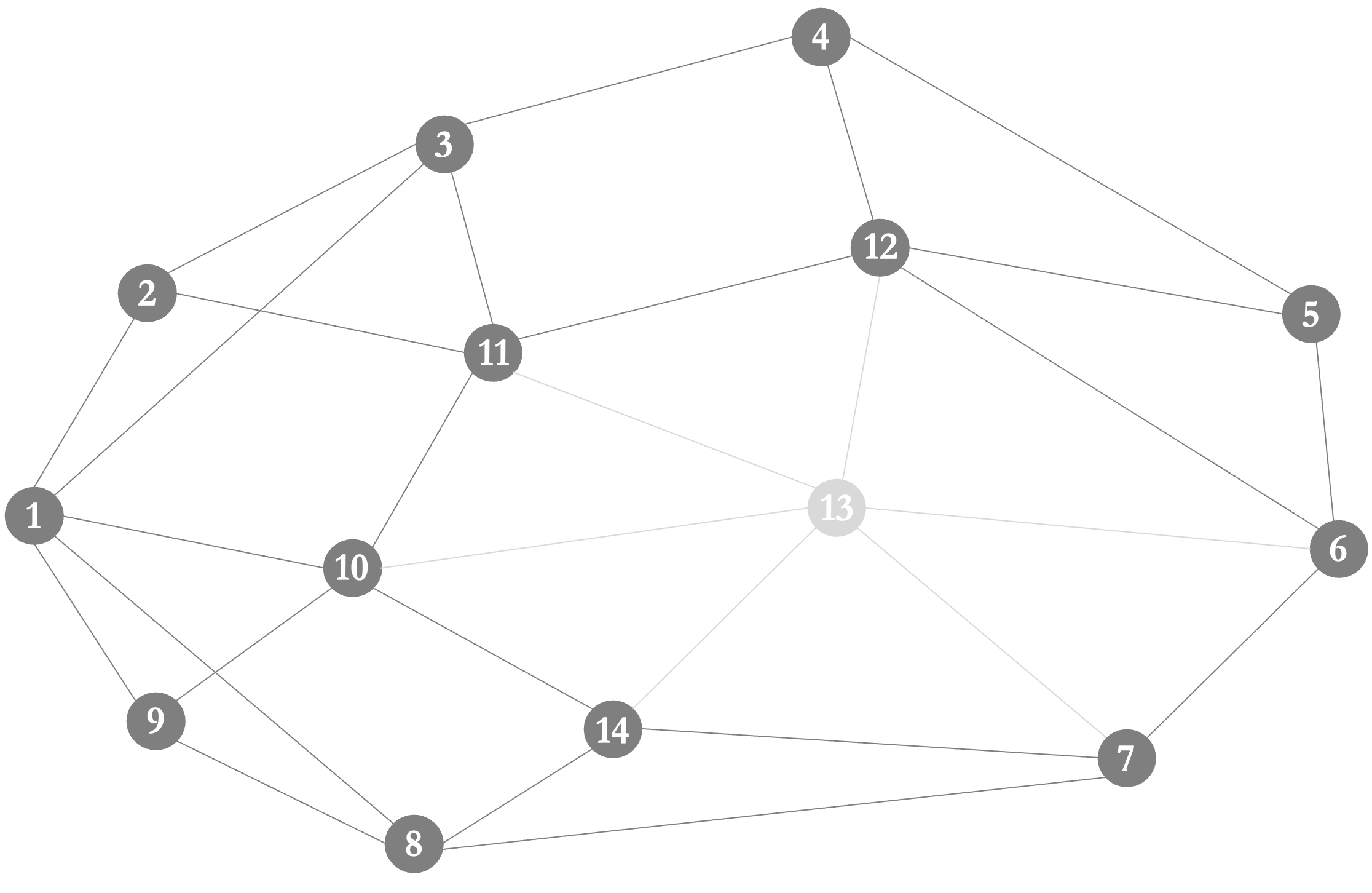
In Figures 4, 5 and 6 some of the introduced concepts are visualized through examples. The graph with nodes in Figure 4 is a -core. Indeed, every node has degree at least . The subgraph induced by the set is a -subcore, i.e., is a set of nodes such that the degree of is three, but its cardinality is not maximum. Assume that we want to determine the Collapsed 3-core Problem on this graph with budget , i.e., we can remove one node only. Two possible feasible solutions of this Collapsed -core Problem are represented in Figure 5 and Figure 6. The first one in Figure 5, which consists in removing node from the graph, leads to a -core of cardinality (no node follows node , because no node has less than neighbors in the remaining graph). The second one in Figure 6, which consists in removing node from the graph, leads to a better solution, since the obtained -core after the cascade effect following node removal consists in nodes. In fact, this is the optimal solution of the Collapsed -core Problem for the graph in Figure 4.



In the rest of this section, we propose three formulations for the problem: the first one relies on the iterative process used to determine the collapsed -core, after the removal of the nodes; the other two formulations are bilevel formulations, considering two agents, a leader who selects the nodes to remove and a follower who computes the resulting -core, solving either formulation (3) or (11). The bilevel structure of the problem comes from the fact that the -core is defined as the induced subgraph with all nodes having degree at least of maximum size. Given that, the aim of the problem is to find the set of nodes to remove, such that the maximal induced -subcore is of minimum cardinality.
5.1 Time-Dependent Formulation
In this section, we describe a “natural” ILP formulation for the Collapsed -Core Problem. This formulation models the so-called cascade effect deriving from the removal of nodes, which are removed at time . At each deletion round (corresponding to a time instant ), all the nodes the degree of which becomes less than are removed from the graph. Assuming that the problem instance is feasible, i.e., that the considered graph has at least nodes, the deletion rounds are at most .
We introduce the binary variables , defined for each node and time , such that:
In the example shown in Figure 6, e.g., and for while, as shown in Figure 6f, for and for , where .
The Collapsed -Core Problem can be formulated as:
| (12a) | |||||
| s.t. | (12b) | ||||
| (12c) | |||||
| (12d) | |||||
| (12e) | |||||
where . The objective function minimizes the number of nodes remaining in the last time instant . The first constraint (12b) imposes that at the beginning (first time instant) exactly nodes are removed. Constraints (12c) state that, if node is not in the graph at time , it cannot be in the graph at time . Finally, constraints (12d) ensure that, if the node is not removed at time 0, it must stay in the graph at time iff more than of its neighbors “survived” at time . Constraint (12d), for a given , and a given , imposes that
- •
if the node is not a collapser, i.e., it is not removed at time 0, and thus
- •
and , i.e., (with )
then is set to 1. The term is thus needed to guarantee that, for the collapsers, the constraints (12d) are still satisfied. For these nodes indeed and will be 0.
The obtained ILP formulation is polynomial in size and can be solved using existing state-of-the-art solvers. It is indeed a compact formulation, which is the main advantage of this first natural approach. However, because of time index , the number of variables is large, thus requiring a long computational time to be solved. For this reason, we present in the following sections two alternative formulations for the Collapsed -Core Problem.
5.2 A first bilevel formulation
In this section, we formulate the Collapsed -Core Problem using bilevel programming where the leader aims at minimizing the cardinality of the -core obtained by removing exactly nodes. The follower instead aims at detecting the -core obtained after the removal of the nodes chosen by the leader, which corresponds to finding the maximal induced subgraph where all the nodes have degree at least . The follower’s problem is modeled as in (3), with additional linking constraints imposing that the -core is computed in the graph resulting after the removal of nodes by the leader.
We consider the upper-level binary variables and the lower-level binary variables (already defined in Eq. (1)), both defined for each node :
Variable is 1 iff node is a collapser. We remark that it corresponds to in the time-dependent formulation (12), presented in Subsection 5.1. Variable , instead, is 1 iff node is in the resulting -core, thus corresponds to in the time-dependent formulation (12).
The set of all possible leader’s policies (removing exactly nodes) is
| (13a) |
Let denote the set of all subsets such that , i.e., . There is a one-to-one correspondence between each element and its incidence vector . The set of all possible nodes subsets inducing -subcores of is defined in Subsection 4.1. If no node is interdicted by the leader, the problem of the follower corresponds to finding the -core in the original graph, defined in Subsection 4.1. The resulting Collapsed -Core Problem can be formulated as the following bilevel problem:
| (14) |
Constraints exclude from the -core the collapsers. Problem (14) does not consider the optimal solutions of the follower’s problem, but only its optimal objective function value. Thus, we do not need to distinguish between optimistic and pessimistic concepts.
5.2.1 Sparse Formulation
Formulation (14) exhibits the structure of so-called interdiction problems, which is a well-known class of bilevel optimization problems (see Kleinert et al. 2021; Smith and Song 2020 for recent surveys on interdiction problems). This structure allows us to apply a Benders-like reformulation technique in which we project out the lower-level variables, and introduce an auxiliary integer variable to represent the objective value of the lower-level problem. We refer to this formulation as sparse, because it is given in the natural space of variables (required to describe the removed set of nodes) and a single auxiliary variable. We start by reformulating the problem (14) as follows:
| (15a) | ||||
| s.t. | (15b) | |||
| (15c) | ||||
Following the ideas from e.g., Wood 2011; Fischetti et al. 2019; Leitner et al. 2022, we can then reformulate (15b), given sufficiently large for all , as:
| (16) |
which is equivalent to the following Benders-like constraints:
| (17) |
In terms of sets inducing the -subcores of , we can rewrite Ineqs. (17) as
| (18) |
The value of needs to be set in such a way that, for a given , in case node (possibly together with some other nodes from ) is interdicted, the value gives the lower bound on the size of the -core of . Since, in the extreme case, the interdiction can lead to an empty -core, we set , resulting into
| (19) |
Alternatively, since the upper-level decisions are binary, we can reformulate constraint (15b) using the following many no-good-cuts:
| (20) |
Indeed, for any given , the cardinality of the -core , when the nodes from are removed by the leader, provides a valid lower bound on . If at least one of the nodes in is not a collapser, the related constraint of type (20) turns out to be redundant, since the right hand side becomes less than or equal to 0.
5.3 A second bilevel formulation
In this section, we propose an alternative bilevel formulation by considering lower-level variables defined in (4), complementary with respect to variables , and formulating the lower-level problem as in (11).
We recall that represent the lower-level variables identifying the nodes not belonging to the collapsed -core of the graph:
We remark that variable corresponds to in the former bilevel formulation. Indeed, in the example shown in Figure 6, for , and for .
The problem of detecting the -core of the graph, given a leader’s decision , can be modelled as the problem of determining the set of nodes outside of the -core:
| (22a) | |||||
| s.t. | (22b) | ||||
| (22c) | |||||
| (22d) | |||||
This formulation differs from formulation (5) only for constraints (22c), which state that a node cannot be in the -core if it is interdicted/removed. Note that problem (22) may be equivalently written as a maximization problem, with objective function , as in (5a).
The corresponding bilevel formulation of the Collapsed -Core Problem is:
| (23a) | ||||
| s.t. | (23b) | |||
| (23c) | ||||
The objective function expresses the fact that we want to find the minimal collapsed -core, computed by solving
In Subsection 4.2, we proved that problem can be reformulated as the following LP formulation:
| (24a) | |||||
| s.t. | (24b) | ||||
| (24c) | |||||
| (24d) | |||||
| (24e) | |||||
| (24f) | |||||
The addition of constraints (24e), indeed, has no impact on the proof of Theorem 1. Since formulation (24) is linear in the variables , and , we can replace it by its dual, as detailed in the following section.
5.3.1 Compact nonlinear formulation
An approach to deal with the bilevel formulation (23) consists in dualizing the lower level continuous formulation (24). Let us define the following dual variables for all : associated with the constraints (24b); associated with the constraints (24c); associated with the constraints (24d); associated with the constraints (24e); associated with the constraints
The dual of the lower-level problem (24) is:
| (25a) | ||||
| (25b) | ||||
| (25c) | ||||
| (25d) | ||||
| (25e) | ||||
For any value of , problem (24) (i) admits at least one feasible solution, (ii) is bounded because both variables and are bounded. Thus, strong duality holds between problem (24) (the LP relaxation of ) and its dual (25). Given what we discussed before, in (23), we can replace by its linear relaxation (24) since their optimal values are the same as proved in Theorem 1, and then replace problem (24) by (25), since their optimal values are the same by strong duality. We can further drop the maximum operator, obtaining the following single-level formulation:
| (26a) | ||||
| s.t. | (26b) | |||
| (26c) | ||||
| (26d) | ||||
| (26e) | ||||
This single-level formulation is a Mixed-Integer Nonlinear Programming (MINLP) problem, that has bilinear terms in (26b), given by . One could linearize these bilinear terms using again McCormick reformulation, and/or applying other specialized techniques. However, most of the these state-of-the-art techniques are integrated in modern MINLP solvers, thus we decided to hand over the compact model (26) as it is to the solver used in the experiments (see Section 8 for details).
6 Valid inequalities
In this section, we describe different classes of valid inequalities, which are used to strengthen the single-level formulations presented above. Some of them are valid for all the feasible solutions, while others cut off parts of the feasible domain due to symmetries or dominance conditions. We point out that an initial pre-processing procedure is applied to which consists of removing all nodes not belonging to its -core.
6.1 Dominance and symmetry breaking inequalities
For any node , we can compute the -core of and define as the set of nodes, including itself, which leave the graph when node is removed (say, the followers of , not to be confused with the follower agent solving the lower level):
In the example graph in Figure 4, as shown in Figures 5 and 6, with , while . Using these sets, defined for each node in the graph, we can add dominance inequalities to our formulations. In the same example as before, and we can observe that , meaning that every node that leave the network when node 3 is removed, would also leave the network when node 1 is removed. In general, if , i.e., the set of followers of node is strictly contained in the set of followers of node , node should be removed first. This can be imposed adding to the time-dependent formulation (12) the following inequalities:
| (27) |
which corresponds to adding the following inequalities to formulations (21), and (26):
| (28) |
An additional family of valid inequalities is related to breaking symmetries among nodes which have the same set of followers. Let be an inclusion-wise maximal subset of nodes such that for all , i.e., contains all the nodes of the graph having a given set of followers, and there exist no superset of the nodes of which have the same set of followers. For example, in the graph in Figure 4, when , nodes and have the same set of followers which is (if leaves the network, leaves it too and vice versa), thus a possible set is . Let the indices , with , be given in increasing order. Then we can break the symmetries by imposing that the node with the lowest index is removed first, i.e.,
| (29) |
for the time-dependent formulation (12), and
| (30) |
6.2 Valid inequalities to consider the cascade effect
We present in this section a family of valid inequalities, related to the nodes which leave the network as a consequence of a single node or a set of nodes leaving. Such inequalities can be added to both the time-dependent formulation (12) and the leader’s problem of the two bilevel formulations.
For any node , we can compute the -core of and the set of followers . Given that by removing , all nodes in will be removed as well, we can add a valid inequality stating that at most one node should be removed from , that is:
| (31) |
for the time-dependent formulation, and
| (32) |
Indeed, if there exists a feasible solution such that is not a collapser, but some of its followers are, i.e., and for some , then there exists an alternative solution with an objective value which is at least as good as the one of the former solution, where is the only collapser in . Such a solution can be obtained by replacing all collapsed nodes by , resulting in at least the same number of leaving nodes.
We assume that the removal of less than nodes (together with the related followers) is not enough to empty the network. Under this assumption, Ineqs. (12b), (15c), (23c), requiring that exactly nodes are removed, as well as Ineqs. (19) and (20), remain still valid when introducing constraints (31) and (32). If instead this condition is not satisfied, then inequalities (31) and (32) are no longer valid. We note that in social networks applications, this assumption is typically satisfied as .
Inequalities (31) and (32) can be generalized to the case in which more than a single node is removed. Let , with , be such set of nodes. Assume
holds, i.e., in the remaining -core there are enough nodes to remove according to the budget left. The set of followers of (including ) can be defined as follows
and the inequality (31) is generalized into:
| (33) |
while the inequality (32) into:
| (34) |
The number of constraints (31) and (32) is equal to the number of nodes in the graph. For each node , the set , i.e., the followers of , can be easily obtained by computing the -core of and the related constraint can be added to the model. Instead, the number of constraints (33) and (34) is . Thus a separation routine is required.
6.3 Lower bound on the solution value
Let be a series of layers, each one containing the nodes of with coreness equal to , with being at least and at most , where is the maximum coreness of any node in the graph. For instance, in the graph in Figure 1, with , we have , contains the cyan nodes, contains the green nodes, while contains the orange nodes.
Let us consider the -core , where . Even by removing any subset of nodes from such -core, the remaining nodes still constitute a -core. The size of the remaining -core is a valid lower bound to the solution value of the Collapsed -Core Problem. Let us denote as this lower bound. This means that we can restrict the set of the incident vectors of all the -subcores of the graph (over which we optimize the lower-level problem) as follows:
| (35) |
Indeed the number of nodes which are not in the feasible -cores belonging to the layers will not be greater than the budget .
This corresponds to adding the following constraint to the time-dependent model (12)
| (36) |
Furthermore, a tighter upper bound on the number of deletion rounds can be defined as .
According to the defined lower bound, in a similar fashion as it is done in stochastic integer programming (see, e.g. Laporte and Louveaux 1993), we can also tighten the constraints of the sparse formulation (21), presented in Section 5.2.1. Inequalities (19) can be restated as follows:
| (39) |
and inequalities (20) as follows:
| (40) |
6.4 Valid inequalities derived from -subcores
For a given , assume that (the degree of nodes in the subgraph of induced by is at least ). Assume we are given an interdiction policy such that at most one of the nodes in is interdicted, then we have that Thus we can impose:
| (41) |
in formulation (21).
This can be easily generalized to the case in which as follows:
| (42) |
This means that, if at most nodes are removed from , then the objective function value is lower bounded by . Indeed, the nodes of the -subcore which remain in the network will still have more than neighbours.
7 Separation procedures
The inequalities (27), (28), (29), and (30) introduced in Subsection 6.1, as well as the inequalities (31) and (32) modeling the cascade effect following the leaving of a single node, introduced in Subsection 6.2, and the ones related to the combinatorial lower bound , i.e., (36), (37) and (38), introduced in Subsection 6.3, are added to the corresponding models during the initialization phase as they are in polynomial number. Specifically, we add the following inequalities: the inequalities (31), or (32), and the inequality (36), or (37), or (38) (just one inequality for each model). As regards inequalities (27), (28), (29), and (30), we add them from the beginning following an heuristic procedure here described. After computing the set of followers for each node , a dominance inequality of type (27) or (28) is added to the corresponding formulation for each node such that . Similarly, a partitioning of the set of nodes into at most disjoint subsets is constructed, by iteratively assigning each node to the subset which contains nodes having exactly the same followers of node . Formally, for any in and . Hence, a symmetry breaking inequality of type (29) or (30) is added to the appropriate formulation for each set of the partition .
Instead, the other valid inequalities introduced in Section 6 need a procedure to be separated. In this section, we first present the separation procedure associated with compact formulations (12) and (26) and used to separate cuts (33) and (34). We then describe the separation procedures for the non-compact formulation (21) used to separate constraints (39), (40) and inequalities (34), and (42). We note that separation is made on integer solutions only by using the specific lazyconstraints separation procedure provided by the commercial solver used in the experiments (Gurobi, in our case). Note that we decided to separate these inequalities on integer solutions only in order to avoid too many calls of the separation procedure (on fractional solutions) and speed-up the solution process.
7.1 Separation procedures for the compact formulations
A heuristic procedure for detecting violated inequalities (34) added to formulation (26) is here described.
- 1.
Consider an interdiction policy of the leader and let denote the related set of collapsers;
- 2.
Given a set of collapsers, this routine is able to identify violated constraints of type (34) where is given by the set of collapsers excluding exactly one of them.
7.2 Separation procedures for the single-level formulation (21)
In the following, we explain how to heuristically separate constraints (34), (39), (40) and (42). The procedure to separate (34) is the same as the one described above. We repeat it here for the ease of reading.
We start initializing the relaxation of problem (21), obtained by dropping constraints (19) and (20). Then, every time a feasible integer solution of such relaxation is found, we compute the corresponding and:
- 1.
For each node do the following:
- (a)
Compute the -core of , i.e., ;
- (b)
If , i.e., , add a violated inequality of type (34) with .
- (a)
- 2.
- 3.
- 4.
Set , and iteratively perform the following steps:
- (a)
Select a node to remove and set ;
- (b)
Compute the -core of ;
- (c)
If , and add a cut of the family (39) with . Otherwise, go to step 5.
- (d)
If is over a given threshold, go to step 5.
- (a)
- 5.
For :
- (a)
consider the set of nodes of having coreness at least .
- (b)
If , then add cut (42).
- (a)
At step 1 of the above presented procedure, we check if the collapsers are all really useful. Indeed, we verify whether each is a follower of the other nodes in ; if this is the case, removing is not useful for the leader: it will anyway disappear as follower of the other collapsers.
At step 2, we verify if it is needed to perform step 3. Indeed, if at least one of the inequalities (34) has been added to the relaxation, there is no need to cut off the current solution by means of (39) and (40), being this solution already excluded by adding constraints of type (34).
At step 4, we add a certain number (at most ) of Bender’s like cuts of type (39) with of increasingly smaller dimension. In order to obtain diversified sets of valid inequalities, nodes in are selected in each iteration of step 4 according to decreasing order of the number of previously added constraints in which they are involved. This heuristic selection procedure means that the more a node is involved in the previous steps, the less it will be considered in step 4.
8 Numerical experiments
In this section, we analyse the computational performance of the following four exact approaches:
- •
- •
- •
- •
Bilevel Solver, corresponding to the bilevel formulation (15) which is solved using a general purpose intersection-cut based solver for Mixed-Integer Bilevel Linear Problems proposed in (Fischetti et al. 2017).
On the one hand, the two compact formulations (12) and (26) are solved using a state-of-the-art MINLP solver together with the separation procedures proposed in Subsection 7.1. On the other hand, formulation (21) is solved using a Branch&Cut method which iteratively builds the feasible set of the original bilevel formulation (15), by adding cuts of type (19), (20) as well as separating the inequalities proposed in Section 6 through the separation procedure illustrated in Subsection 7.2. The bilevel formulation (15) is instead solved as it is through the general purpose algorithm proposed in (Fischetti et al. 2017).
The proposed formulations were implemented in Python 3.8 and solved by using the Gurobi solver (version 9.5.2). The bilevel solver of Fischetti et al. 2017 uses Cplex 12.7. The separation procedures presented in the paper are implemented within lazy callbacks, with the threshold on used in step 4d of separation procedure presented in Subsection 7.2 set to 10, and set to .
All the experiments were conducted in single-thread mode, on a 2.3 GHz Intel Xeon E5 CPU, 128 GB RAM. A time limit of two hours of computation and a memory limit of 10 GB were imposed for every run.
8.1 Benchmark Instances
In order to test and compare the performances of the discussed methods, a set of 136 instances was arranged starting from 14 different networks collected from the literature. All the instances files are collected in the online public repository https://bit.ly/collapsed-k-core.
For each network, several combinations of values for and were selected by analysing the core number distribution of the nodes. Table 1 reports, for each network, the bibliographic source from which it was collected, the number of its nodes, the number of its edges, the different selected values for , as well as the associated sizes of the network (nodes and edges) after pre-processing and, finally, the selected values for the budget .
| network | #nodes | #edges | k | #nodes after pre-processing | #edges after pre-processing | budget |
| adjnoun (Newman 2006) | 112 | 425 | 5 | 63 | 298 | {3} |
| 4 | 79 | 359 | {3, 4, 5} | |||
| 3 | 89 | 389 | {3, 4, 5} | |||
| 2 | 102 | 415 | {3, 4, 5} | |||
| as-22july06 (University of Oregon 2004) | 22963 | 48436 | 15 | 168 | 3115 | {3, 4, 5} |
| 10 | 322 | 4845 | {3, 4, 5} | |||
| 5 | 1087 | 9493 | {3, 4, 5} | |||
| astro-ph (Newman 2001) | 16706 | 121251 | 42 | 400 | 10552 | {3, 4, 5} |
| 32 | 936 | 23433 | {3, 4, 5} | |||
| 28 | 1393 | 32375 | {3, 4, 5} | |||
| cond-mat (Newman 2001) | 16726 | 47594 | 9 | 943 | 6573 | {3, 4, 5} |
| 8 | 1487 | 9544 | {3, 4, 5} | |||
| 7 | 2227 | 13280 | {3, 4, 5} | |||
| 6 | 3442 | 18713 | {3, 4, 5} | |||
| cond-mat-2003 (Newman 2001) | 31163 | 120029 | 13 | 1132 | 12732 | {3, 4, 5} |
| 12 | 1609 | 17327 | {3, 4, 5} | |||
| 10 | 2901 | 28339 | {3, 4, 5} | |||
| 9 | 4071 | 36920 | {3, 4, 5} | |||
| cond-mat-2005 (Newman 2001) | 40421 | 175692 | 14 | 1793 | 24595 | {3, 4, 5} |
| 13 | 2151 | 28640 | {3, 4, 5} | |||
| 12 | 2808 | 35214 | {3, 4, 5} | |||
| 11 | 3555 | 42346 | {3, 4, 5} | |||
| dolphins (Lusseau et al. 2003) | 62 | 159 | 4 | 36 | 109 | {3} |
| 3 | 45 | 135 | {3, 4, 5} | |||
| 2 | 53 | 150 | {3, 4, 5} | |||
| football (Girvan and Newman 2002) | 115 | 613 | 8 | 114 | 606 | {3, 4, 5} |
| 7 | 115 | 613 | {3, 4, 5} | |||
| hep-th (Newman 2001) | 8361 | 15751 | 7 | 137 | 885 | {3, 4, 5} |
| 6 | 358 | 1847 | {3, 4, 5} | |||
| 5 | 851 | 3775 | {3, 4, 5} | |||
| 4 | 1735 | 6552 | {3, 4, 5} | |||
| karate (Zachary 1977) | 34 | 78 | 2 | 33 | 77 | {3, 4, 5} |
| lesmis (Knuth 1993) | 77 | 254 | 6 | 38 | 186 | {3, 4, 5} |
| 4 | 41 | 197 | {3, 4, 5} | |||
| 3 | 48 | 215 | {3, 4, 5} | |||
| 2 | 59 | 236 | {3, 4, 5} | |||
| netscience (Newman 2006) | 1589 | 2742 | 5 | 247 | 976 | {3, 4, 5} |
| 4 | 470 | 1511 | {3, 4, 5} | |||
| 3 | 751 | 2045 | {3, 4, 5} | |||
| 2 | 1141 | 2535 | {3, 4, 5} | |||
| polbooks (Krebs 1999) | 105 | 441 | 5 | 65 | 300 | {3, 4} |
| 4 | 98 | 422 | {3, 4, 5} | |||
| 3 | 103 | 437 | {3, 4, 5} | |||
| 2 | 105 | 441 | {3, 4, 5} | |||
| power (Watts and Strogatz 1998) | 4941 | 6594 | 4 | 36 | 106 | {3, 4, 5} |
| 3 | 231 | 479 | {3, 4, 5} | |||
| 2 | 3353 | 5006 | {3, 4, 5} |
8.2 Effectiveness of the Collapsed -Core formulations
The detailed results obtained by testing the four methods on the instances described in Subsection 8.1 are available online at https://bit.ly/collapsed-k-core. In the following, we report summary tables and charts which we use to compare the tested methods and formulations. Because of the imposed memory limits, the Time-Dependent Model solves only for 87 instances while, for the remaining 48, even the relaxation at the root node is not solved. For this reason, we summarize in Table 2 the results obtained by testing the four methods on this subset of 87 instances, reporting for each of them: #opt, the number of optimal solutions found by the method within the limits; LB, the average lower bound; UB, the average upper bound; [%], the average percentage gap, where the gap is calculated as per each instance; time[s], the average computing time in seconds; B&C nodes, the average number of nodes of the branch-and-cut tree at termination; , the average lower bound computed by solving the relaxation at the root node; [%], the average gap with respect to the best known solution (dimension of the -core), calculated as per each instance; [%], the average percentage gap with respect to the root bound, calculated as per each instance.
#opt LB UB [%] time[s] B&C nodes [%] [%] Time-Dependent Model 29 84.6 207.0 41.2 5234 79084 68.7 4.66 71.5 Sparse Model 44 102.5 207.4 30.5 4045 30508 81.6 1.91 70.8 Nonlinear Model 52 112.3 201.7 20.4 3347 1110881 81.6 0.38 70.4 Bilevel Solver 26 23.1 212.1 55.8 5297 18263 2.67 4.68 96.5
The results show a clear superiority of the Nonlinear Model, both in terms of time and solution quality. Indeed, the Nonlinear Model provides the highest number of optimal solutions among the tested methods, yielding 52 out of 87 instances solved to optimality. Furthermore, the average computing time required by the Nonlinear Model is considerably lower than the one required by the other formulations; also, the provided average final lower and upper bounds values and gaps are tighter. Specifically, the lower bound computed in the preprocessing procedure is on average. The improvement with respect to this value is much higher for the Nonlinear Model than for the other approaches which take this lower bound into account (i.e., all the approaches, but the bilevel solver). On average, the number of nodes explored by the branch-and-cut approach solving the Nonlinear Model is greater than the number of nodes explored by the one solving the Sparse Model and the number of nodes explored by the Bilevel Solver. This reflects the fact that the problems considered at each node of the branch-and-cut tree solving the Nonlinear Model are easier to solve with respect to the ones of the other models, so that, in the same amount of time, more nodes are explored.
All the three proposed problem-specific methods exhibit better performing behaviors than the general purpose Bilevel Solver. To better visualize this computational dominance, three summary charts related to the four methods solving the considered 87 instances are reported in B.
Since the imposed memory limits prevented the Time-Dependent Model from solving the remaining instances, from now on we restrict the comparison to the other three methods and consider the whole instance set described in Subsection 8.1. In particular, in Table 3, we report the same information as in Table 2, but this time for the whole set of 136 instances, with respect to the three following methods: Sparse Model, Nonlinear Model and Bilevel Solver.
#opt LB UB [%] time[s] B&C nodes [%] [%] Sparse Model 44 266.8 911.4 46.3 5182 21919 253.3 1.89 72.1 Nonlinear Model 52 274.0 892.8 39.6 4735 744905 253.3 0.04 71.6 Bilevel Solver 26 22.4 915.9 71.3 5984 11892 3.80 3.76 97.7
The results on the whole set of instances confirm the computational dominance of the Nonlinear Model, which solves 52 out of the 136 instances to optimality and almost always provides solution values which are better than or equal to the ones found by the other methods, with an average gap of 0.04%, computed with respect to the best known feasible solutions. Again, the number of branch-and-cut nodes reflects the faster resolution of the continuous relaxation of the Nonlinear Model at branching nodes.
We further provide three summary charts related to the three methods solving all the 136 instances. The first chart, shown in Figure 7, reports the number of instances solved to optimality within a given computational time. The second one, in Figure 8a, shows the optimality gap at termination, i.e., what we called [%]. In particular, the plot shows the number of instances (on the vertical axis) for which the gap at termination is smaller than or equal to the value reported on the horizontal axis. Figure 8b reports the gap between the feasible solution at termination, and the best found feasible collapsed -core among the three compared approaches, i.e., what we called [%]. Again, the chart shows the number of instances (on the vertical axis) for which the value of is smaller than or equal to the value reported on the horizontal axis.


Overall, all the three charts show that the two approaches proposed in this paper are much more effective than the bilevel solver, which is largely outperformed by each of them. In the first chart (Figure 7), it can be observed that, only when the computational time is strictly below 20 seconds, the number of instances solved to optimality by the Sparse Model is slightly greater than the number of instances solved to optimality by the Nonlinear Model. However, when the considered time is larger than 20 seconds, the Nonlinear Model dominates the other two approaches. The chart in Figure 8a demonstrates that the Nonlinear Model produces a gap at termination which is always lower than the one returned by the other approaches. Finally, Figure 8b shows that, for more than 130 instances out of 136, the Nonlinear Model produces the best feasible solution, and, for the remaining 4 instances, the gap with respect to the best feasible solution found by one of the other models is below 3%. Concerning the Sparse Model, it returns the best feasible solution for about 50 instances, and the gap for the remaining instances is less than 17%. Finally, the bilevel solver finds the best feasible solution only for about 30 instances out of 136, and a gap with respect to the best one can be as high as 25%.
We also made an additional set of tests to verify the effectiveness of the valid inequalities presented in Section 6. Specifically, we used model (21) as a benchmark and tested the following configurations:
(i) without any valid inequalities; (ii) with symmetry breaking inequalities (28), (30), and lower bound constraint (37); (iii) with symmetry breaking inequalities (28), (30), lower bound constraint (37), followers’ inequalities (32) added to the formulation from the beginning, and constraints (34) separated during the B&C; (iv) with symmetry breaking inequalities (28), (30), lower bound constraint (37), and constraints (39) separated during the B&C; (v) with symmetry breaking inequalities (28), (30), lower bound constraint (37), and constraints (42) separated during the B&C; (vi) the Sparse Model with all the introduced valid inequalities (i.e., the model considered in the comparisons with the other models above).Results are summarized in Table 4 where we report, for each tested configuration: the number of optimal solutions found (#opt), the average percentage gap at termination (gap[%]), the average computing time (time[s]), the number of branch-and-cut nodes (B&C nodes), and the number of added inequalities: (28), (30), (32), (34), (39), and (42), respectively.
| Model | #opt | gap[%] | time[s] | B&C nodes | #(28) | #(30) | #(32) | #(34) | #(39) | #(42) | |
|---|---|---|---|---|---|---|---|---|---|---|---|
| (i) | Model (21) | 24 | 82.4 | 6093 | 6388 | 0 | 0 | 0 | 0 | 0 | 0 |
| (ii) | Model (21) + (28) + (30) + (37) | 27 | 56.2 | 5955 | 5356 | 1221 | 144 | 0 | 0 | 0 | 0 |
| (iii) | Model (21) + (28) + (30) + (37) + (32) + (34) | 29 | 55.3 | 5847 | 6260 | 1221 | 144 | 303 | 242 | 0 | 0 |
| (iv) | Model (21) + (28) + (30) + (37) + (39) | 44 | 47.5 | 5132 | 16545 | 1221 | 144 | 0 | 0 | 131068 | 0 |
| (v) | Model (21) + (28) + (30) + (37) + (42) | 29 | 53.0 | 5907 | 23465 | 1221 | 144 | 0 | 0 | 0 | 51895 |
| (vi) | Sparse Model | 44 | 46.3 | 5182 | 21919 | 1221 | 144 | 303 | 183 | 91226 | 12631 |
As expected, the number of optimal solutions found, as well as the average percentage gap at termination improve when adding further valid inequalities to the basic model (21). We can also notice that the average time does not increase when increasing the number of considered valid inequalities. Inequalities (39) turn out to be the most effective, leading to 44 optimal solutions (and an average gap of 47.1%), as many as the ones found by the complete Sparse Model (with an average gap of 46.3%). The average number of added inequalities (28), (30), and (32) is constant for all configurations since they are not separated, but added to the model from the beginning, together with the lower bound constraint (37).
Finally, we provide two sensitivity analysis tables in which we group instances into three groups: Small (with ), Medium (with ) and Large (with ), where is the number of nodes of the network after the pre-processing procedures. For each group, we consider three values of the budget , thus obtaining nine classes of instances. For each class, we report in Tables 5 and 6 the total number of instances in the class (#total). In Table 5, for each method we report the number of instances solved to optimality (#opt), the average computing time in seconds (time[s]) and the average number of nodes of the branch-and-cut tree (B&C nodes); additionally, for the Sparse Model, we also report the average number of added cuts. In Table 6, instead, we report for each class [%], [%], and [%].
The reported values show how increasing the value of the budget affects the different methods. As expected, when the value of increases, the number of instances solved to optimality decreases for each method, while the average solution time and the average gap value increase. Specifically, all the instances of the first class, i.e., small instances with , are solved to optimality by both the Sparse and Nonlinear models, while the Bilevel Solver provides the optimal certified solution for all except two of them. The Nonlinear Model solves to optimality also all the instances of the second class, i.e., small instances with . For the remaining classes, instead, no method is able to certify the optimality of all the instances from a given subclass. In particular, no optimal solution is found for any of the instances from the group “large”, within the imposed time limit. Overall, this analysis shows that the difficulty of an instance is highly affected by the budget value, in addition to the network size, but, for non-large instances, the Nonlinear Model confirms its superiority with respect to the remaining approaches.
Class details Sparse Model Nonlinear Model Bilevel Solver size b #total #opt time[s] B&C nodes cuts #opt time[s] B&C nodes #opt time[s] B&C nodes 3 14 14 102 5481 1719 14 27.6 26633 12 1623 10455 4 12 11 1296 31205 5409 12 242 332382 7 3574 32115 Small 5 11 6 3820 53377 9226 10 1413 1960571 4 4805 45443 3 17 9 4445 23730 16602 9 3961 353716 1 6884 11410 4 17 3 6431 34573 19101 6 5544 1381271 1 6863 10923 Medium 5 17 1 6777 39951 16420 1 6938 2460756 1 6817 10669 3 16 0 7200 5750 11795 0 7200 90644 0 7200 573 4 16 0 7200 4393 9417 0 7200 80239 0 7200 492 Large 5 16 0 7200 6881 6206 0 7200 82350 0 7200 474
Class details Sparse Model Nonlinear Model Bilevel Solver size b #Total [%] [%] [%] [%] [%] [%] [%] [%] [%] 3 14 0.00 75.1 0.00 0.00 75.1 0.00 7.40 92.5 0.28 4 12 6.40 82.4 0.11 0.00 82.4 0.00 20.2 95.6 1.28 Small 5 11 34.5 87.7 1.40 3.10 87.7 0.00 34.4 97.2 2.19 3 17 22.4 57.3 0.46 22.6 57.1 0.17 78.0 97.0 5.35 4 17 50.5 65.5 2.52 34.2 64.9 0.12 84.2 97.9 6.89 Medium 5 17 66.5 73.3 3.43 56.5 72.5 0.00 85.8 99.0 7.87 3 16 64.0 64.0 2.14 63.0 63.1 0.00 98.8 99.7 2.06 4 16 73.4 73.4 2.69 72.3 72.4 0.00 99.1 99.8 2.62 Large 5 16 79.8 79.8 3.38 78.9 78.9 0.00 99.5 99.9 3.22
9 Conclusion
Identifying the most critical users, in terms of network engagement, is a compelling topic in social networks analysis. Users who leave a community potentially affect the cardinality of its -core, i.e., the maximal induced subgraph of the network with minimum degree at least . In this paper, we presented different mathematical programming formulations of the Collapsed -Core Problem, consisting in finding the nodes of a graph the removal of which leads to the -core of minimal cardinality. We started with a time-indexed compact formulation which models the cascade effect following the removal of the nodes. Then, we proposed two different bilevel programming models of the problem. In both of them, the leader aims to minimize the cardinality of the -core obtained by removing exactly nodes. The follower wants to detect the -core obtained after the decision of the leader on the nodes to remove, i.e., finding the maximal subgraph of the new graph where all the nodes have degree at least . The two formulations differ in the way the follower’s problem is modeled. In the first one, the lower level is an ILP model. It is solved through a Benders-like decomposition approach. In the second bilevel formulation, the lower level is modeled through LP, which we dualized in order to end up with a single-level formulation. Preprocessing procedures, and valid inequalities have been further introduced to enhance the proposed formulations.
In order to evaluate the proposed formulations we tested different existing instances, showing the superiority of the single-level reformulation of the second bilevel model. We further compared the approaches with the general purpose bilevel solver proposed in (Fischetti et al. 2017) which is outperformed by our problem-specific solution methods. The efficiency of the proposed valid inequalities is also demonstrated by performing additional computational experiments.
Interesting directions for future research are related, for example, to applying our approaches to the -core minimization problem through edge deletion (Zhu et al. 2018). Furthermore, other related problems, like the so-called Anchored -core Problem (Bhawalkar et al. 2015) may benefit from the proposed solution techniques.
References
- Batagelj and Zaversnik (2002) Batagelj, V., Zaversnik, M., 2002. An algorithm for cores decomposition of networks. Preprint series of University of Ljubljana 40, 798–806.
- Bhawalkar et al. (2015) Bhawalkar, K., Kleinberg, J., Lewi, K., Roughgarden, T., Sharma, A., 2015. Preventing unraveling in social networks: the anchored -core problem. SIAM Journal on Discrete Mathematics 29 (3), 1452–1475.
- Cerulli (2021)
Cerulli, M., 2021. Bilevel optimization and applications. Ph.D. thesis,
Institut Polytechnique de Paris.
URL http://www.theses.fr/2021IPPAX108 - Chitnis et al. (2013) Chitnis, R., Fomin, F. V., Golovach, P. A., 2013. Preventing unraveling in social networks gets harder. In: Proceedings of the Twenty-Seventh AAAI Conference on Artificial Intelligence. AAAI’13. AAAI Press, pp. 1085–1091.
- Colson et al. (2007) Colson, B., Marcotte, P., Savard, G., 2007. An overview of bilevel optimization. Annals of Operations Research 153, 235–256.
- Dempe (2002) Dempe, S., 2002. Foundations of Bi-Level Programming, 1st Edition. Nonconvex Optimization and Its Applications. Springer US.
- Fischetti et al. (2017) Fischetti, M., Ljubić, I., Monaci, M., Sinnl, M., 2017. A new general-purpose algorithm for mixed-integer bilevel linear programs. Operations Research 65 (6), 1615–1637.
- Fischetti et al. (2019) Fischetti, M., Ljubić, I., Monaci, M., Sinnl, M., 2019. Interdiction games and monotonicity, with application to knapsack problems. INFORMS Journal of Computing 31 (2), 390–410.
- Furini et al. (2022) Furini, F., Ljubić, I., Malaguti, E., Paronuzzi, P., 2022. Casting light on the hidden bilevel combinatorial structure of the capacitated vertex separator problem. Operations Research 70 (4), 2399–2420.
- Furini et al. (2021) Furini, F., Ljubić, I., Segundo, P. S., Zhao, Y., 2021. A branch-and-cut algorithm for the edge interdiction clique problem. European Journal of Operational Research 294 (1), 54–69.
- Furini et al. (2020) Furini, F., Ljubić, I., Malaguti, E., Paronuzzi, P., 2020. On integer and bilevel formulations for the -vertex cut problem. Mathematical Programming Computation 12, 133–164.
- Furini et al. (2019) Furini, F., Ljubić, I., San Segundo, P., Martin, S., 2019. The maximum clique interdiction problem. European Journal of Operational Research 277 (1), 112–127.
- Gillen et al. (2021) Gillen, C. P., Veremyev, A., Prokopyev, O. A., Pasiliao, E. L., 2021. Fortification against cascade propagation under uncertainty. INFORMS Journal on Computing 33 (4), 1481–1499.
- Girvan and Newman (2002) Girvan, M., Newman, M. E. J., 2002. Community structure in social and biological networks. Proceedings of the National Academy of Sciences 99 (12), 7821–7826.
- Kleinert et al. (2021) Kleinert, T., Labbé, M., Ljubić, I., Schmidt, M., 2021. A survey on mixed-integer programming techniques in bilevel optimization. EURO Journal on Computational Optimization 9, 100007.
- Knuth (1993)
Knuth, D. E., 1993. The Stanford GraphBase: A Platform for Combinatorial
Computing. Addison-Wesley Educational, Boston, MA.
URL https://www-cs-faculty.stanford.edu/~knuth/sgb.html - Krebs (1999) Krebs, V., 1999. The Social Life of Books Visualizing Communities of Interest via Purchase Patterns on the WWW. http://orgnet.com/booknet.html [Accessed: 27.10.2022].
- Laishram et al. (2020) Laishram, R., Erdem Sar, A., Eliassi-Rad, T., Pinar, A., Soundarajan, S., 2020. Residual core maximization: An efficient algorithm for maximizing the size of the -core. In: Proceedings of the 2020 SIAM International Conference on Data Mining. SIAM, pp. 325–333.
- Laporte and Louveaux (1993) Laporte, G., Louveaux, F. V., 1993. The integer L-shaped method for stochastic integer programs with complete recourse. Operations Research Letters 13 (3), 133–142.
- Leitner et al. (2022) Leitner, M., Ljubić, I., Monaci, M., Sinnl, M., Tanınmış, K., 2022. An exact method for binary fortification games. European Journal of Operational Research.
- Luo et al. (2021) Luo, J., Molter, H., Suchỳ, O., 2021. A parameterized complexity view on collapsing -cores. Theory of Computing Systems 65 (8), 1243–1282.
- Lusseau et al. (2003) Lusseau, D., Schneider, K., Boisseau, O., Haase, P., Slooten, E., Dawson, S., 2003. The bottlenose dolphin community of doubtful sound features a large proportion of long-lasting associations - can geographic isolation explain this unique trait? Behavioral Ecology and Sociobiology 54, 396–405.
- Malliaros et al. (2020) Malliaros, F. D., Giatsidis, C., Papadopoulos, A. N., Vazirgiannis, M., 2020. The core decomposition of networks: Theory, algorithms and applications. The International Journal on Very Large Data Bases 29 (1), 61–92.
- Matula and Beck (1983) Matula, D. W., Beck, L. L., 1983. Smallest-last ordering and clustering and graph coloring algorithms. Journal of the Association for Computing Machinery 30 (3), 417–427.
- Newman (2001) Newman, M. E. J., 2001. The structure of scientific collaboration networks. Proceedings of the National Academy of Sciences 98 (2), 404–409.
- Newman (2006) Newman, M. E. J., Sep 2006. Finding community structure in networks using the eigenvectors of matrices. Physical Review E 74, 036104.
- Sariyüce and Pinar (2016) Sariyüce, A. E., Pinar, A., 2016. Fast hierarchy construction for dense subgraphs. Proceedings of the Very Large Data Bases Endowment 10 (3), 97–108.
- Seidman (1983) Seidman, S. B., 1983. Network structure and minimum degree. Social Networks 5 (3), 269–287.
- Smith and Song (2020) Smith, J. C., Song, Y., 2020. A survey of network interdiction models and algorithms. European Journal of Operational Research 283 (3), 797–811.
- University of Oregon (2004) University of Oregon, 2004. Route views archive project. http://routeviews.org/ [Accessed: 27.10.2022].
- Vicente and Calamai (1994) Vicente, L. N., Calamai, P. H., 1994. Bilevel and multilevel programming: A bibliography review. Journal of Global Optimization 5 (3), 291–306.
- Watts and Strogatz (1998) Watts, D. J., Strogatz, S. H., Jun 1998. Collective dynamics of ‘small-world’ networks. Nature 393 (6684), 440–442.
- Wood (2011) Wood, R. K., 2011. Bilevel Network Interdiction Models: Formulations and Solutions. John Wiley & Sons, Ltd.
- Yu et al. (2019) Yu, S., Liu, Y., Ren, J., Bedru, H. D., Bekele, T. M., Wan, L., Xia, F., 2019. Mining key scholars via collapsed core and truss. In: 2019 IEEE DASC/PiCom/CBDCom/CyberSciTech Conference. pp. 305–308.
- Zachary (1977)
Zachary, W. W., 1977. An information flow model for conflict and fission in
small groups. Journal of Anthropological Research 33 (4), 452–473.
URL http://www.jstor.org/stable/3629752 - Zhang et al. (2017a) Zhang, F., Zhang, W., Zhang, Y., Qin, L., Lin, X., 2017a. OLAK: An Efficient Algorithm to Prevent Unraveling in Social Networks. Proceedings of the Very Large Data Bases Endowment 10 (6), 649–660.
- Zhang et al. (2017b) Zhang, F., Zhang, Y., Qin, L., Zhang, W., Lin, X., 2017b. Finding critical users for social network engagement: The collapsed -core problem. Proceedings of the AAAI Conference on Artificial Intelligence 31 (1).
- Zhang and Yang (2020) Zhang, J., Yang, Y., 2020. Research on collapsed (, )-NP-community on signed graph. Journal of Physics: Conference Series 1486 (4), 042015.
- Zhu et al. (2018) Zhu, W., Chen, C., Wang, X., Lin, X., 2018. -core minimization: An edge manipulation approach. In: Proceedings of the 27th ACM International Conference on Information and Knowledge Management. CIKM ’18. Association for Computing Machinery, New York, NY, USA, pp. 1667–1670.
Appendix A Notation
Table 7 reports a list of mathematical notations used throughout the paper.
Notation Definition set of nodes of graph set of edges of graph set of neighbors of node minimum degree of graph subgraph of graph induced by the set of nodes subgraph of graph induced by the set of nodes set of incident vectors of any -subcore of graph (Eq. (2)) set of the -subcores of graph -core of graph set of incident vectors of any interdiction policy (Eq. (13a)) set of the interdiction policies set of the followers of node , including itself set of the followers of the nodes in the set including itself
Appendix B Cumulative charts on a set of 87 instances
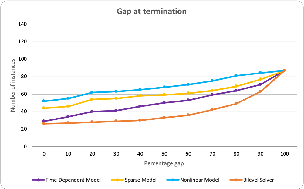
We report here three cumulative charts related to the four methods (Time Dependent Model, Sparse Model, Nonlinear Model, and Bilevel Solver) solving 87 instances. The first chart in Figure 9 reports the number of instances solved to optimality within a given computational time. The second one, in Figure 10a, shows the number of instances solved with a gap at termination which is smaller than or equal to the value reported on the horizontal axis. The last one, in Figure 10b, shows the number of instances for which the value of [%] (the gap between the feasible solution at termination, and the best found feasible solution among the four compared approaches) is smaller than or equal to the value reported on the horizontal axis.