Estimating Reflectance Layer from a Single Image: Integrating Reflectance Guidance and Shadow/Specular Aware Learning
Abstract
Estimating the reflectance layer from a single image is a challenging task. It becomes more challenging when the input image contains shadows or specular highlights, which often render an inaccurate estimate of the reflectance layer. Therefore, we propose a two-stage learning method, including reflectance guidance and a Shadow/Specular-Aware (S-Aware) network to tackle the problem. In the first stage, an initial reflectance layer free from shadows and specularities is obtained with the constraint of novel losses that are guided by prior-based shadow-free and specular-free images. To further enforce the reflectance layer to be independent of shadows and specularities in the second-stage refinement, we introduce an S-Aware network that distinguishes the reflectance image from the input image. Our network employs a classifier to categorize shadow/shadow-free, specular/specular-free classes, enabling the activation features to function as attention maps that focus on shadow/specular regions. Our quantitative and qualitative evaluations show that our method outperforms the state-of-the-art methods in the reflectance layer estimation that is free from shadows and specularities. Code is at: https://github.com/jinyeying/S-Aware-network.
Introduction
Reflectance layer estimation is a fundamental task in computer vision. It is a part of intrinsic image decomposition, which decomposes an input image into the reflectance layer and the shading layer (Barrow et al. 1978). The reflectance layer provides useful information for real-world applications, e.g., surface retexturing (Garces et al. 2012), relighting (Liu et al. 2020a), object compositing (Bi, Han, and Yu 2015). Unfortunately, reflectance layer estimation from a single image is an inherently ill-posed problem.


Several methods have been proposed to deal with the problem. Non-deep learning methods e.g., (Bell, Bala, and Snavely 2014) impose priors on the estimated reflectance layer. Supervised learning methods e.g., (Das, Karaoglu, and Gevers 2022), while effective, still suffer from problems, particularly those related to shadows and specularities. Some existing unsupervised learning methods learn from time-lapse data (Li and Snavely 2018b; Liu et al. 2020a), multi-view data (Yi, Tan, and Lin 2020) or sets of unpaired images (Liu et al. 2020b).
Among these methods, only few consider shadows (Baslamisli et al. 2021a; Baslamisli et al. 2021b) and specular highlights (Yi, Tan, and Lin 2020). However, they suffer from a few drawbacks. First, most of them are trained only on synthesized datasets, and thus their accuracy depends heavily on the quality of the synthesized data. Second, while these methods work well in some cases, they tend to fail in handling large shadow or specular regions, as shown in Fig. 1. Third, most of these methods assume that reflectance changes cause abrupt image intensity changes, while shading changes cause smooth image intensity changes (Land and McCann 1971). However, shadows, which should belong to the shading layer, can also cause abrupt intensity changes in the real world, which goes against this assumption.
In this paper, our goal is to decompose a diffuse reflectance layer that is free from shadows and specularities. To achieve this, we introduce a two-stage network based on reflectance guidance and a Shadow/Specular-Aware (S-Aware) network. The first stage is to obtain an initial diffuse reflectance layer free from shadows and specularities. To achieve this, we introduce novel losses constrained by prior-based shadow-free (Finlayson, Drew, and Lu 2004) and specular-free images (Tan and Ikeuchi 2005).
Once the initial reflectance layer is obtained, we feed it into the S-Aware network, which identifies shadow/specular regions by modulating the activation features as attention maps. To enable the S-Aware network to self-learn the shadow/specular regions, a Shadow/Specularity Classifier (S-Classifier) is employed to distinguish the first-stage estimated reflectance layer from the input image. Specifically, by distinguishing shadows from shadow-free or specularities from specular-free, the activation features form shadow/specular attention. Our attention mechanism modulates the activation weights with encoded features that capture spatially varying regions. Once our network can focus on shadow/specular regions, it can refine the reflectance layer to be free from shadows and specularities. In summary, here are our contributions:
- •
To the best of our knowledge, our method is the first single-image diffuse reflectance layer estimation network that performs robustly even in the presence of shadows and specularities. This differs from existing intrinsic image decomposition methods, which tend to fail to remove shadows and specularities from the reflectance layer.
- •
We introduce a reflectance guidance framework that provides reliable guidance for our network to learn the reflectance layer. Our novel losses constrain the reflectance layer free from shadows and specularities, based on prior-based shadow-free and specular-free images.
- •
We propose an S-Aware network to modulate activation features as shadow/specular attention. Our network automatically learns to focus on these regions, since our S-Classifier distinguishes shadows from shadow-free or specularities from specular-free.
Our quantitative and qualitative evaluations show that our method outperforms the state-of-the-art methods in various datasets for suppressing shadows and specularities in the reflectance layer, including: 4 intrinsic datasets, 2 shadow datasets and 1 specular dataset.

Related Work
Reflectance Layer Estimation The Retinex algorithm (Land and McCann 1971) assumes reflectance changes cause large gradients, while shading variation corresponds to small gradients. Subsequently, various priors, e.g., sparse reflectance, reflectance colors, textures, depth are utilized to regularize the reflectance layer. However, with only hand-crafted constraints, these methods are not adaptive enough, and scene-specific parameters are hard to cover real-world shadows and specularities. Moreover, the assumption that shading changes cause smooth image intensity changes is not likely to cover the large shading change, such as shadow regions.
In recent years, many deep-learning-based methods have been introduced (Garces et al. 2022), and most of them adopt supervised learning (Narihira, Maire, and Yu 2015; Baslamisli, Le, and Gevers 2018; Fan et al. 2018; Das, Karaoglu, and Gevers 2022). The challenge of applying learning-based methods is the lack of a variety of real images with ground truth. Synthetic datasets e.g., (Butler et al. 2012; Shi et al. 2017; Li and Snavely 2018a; Baslamisli et al. 2021a; Han et al. 2022) highly depend on the quality of the rendering techniques and 3D models. Poor rendering quality will make the network fail to handle real images in the testing stage, due to the gaps between the synthetic and real image domains.
Real image datasets e.g., (Grosse et al. 2009; Bell, Bala, and Snavely 2014; Kovacs et al. 2017)) are either too limited, lack diversity, or have highly sparse annotations. To address the limitations of supervised learning methods, a few unsupervised learning methods are proposed. They mainly focus on images with static reflectance and varied illumination (Lettry, Vanhoey, and Van Gool 2018; Ma et al. 2018; Li and Snavely 2018b; Liu et al. 2020a). Unlike multi-image approaches, unpaired translation (Liu et al. 2020b) and internal self-similarity (Zhang et al. 2021) provide more solutions. However, most existing methods have artefacts in the reflectance layer, particularly on the shadow and specular regions. Unlike existing methods, our network estimates the reflectance layer that is free from shadows and specularities.
Shadow and Specularity Removal A few intrinsic image decomposition methods (Baslamisli et al. 2021b; Baslamisli et al. 2021a; Zhang et al. 2021) attempt to address shadows, and other methods (Shi et al. 2017; Yi, Tan, and Lin 2020; Li et al. 2020) attempt to solve specular highlights separation using a large-scale synthetic data in training. However, the accuracy of the rendering limits the performance of the methods on the real-world shadows and specularities.
Note that, there are a few shadow/specularity removal methods that do not decompose the input image to the intrinsic layers, such as (Kawakami, Ikeuchi, and Tan 2005; Jin, Sharma, and Tan 2021; Guo et al. 2023; Jin et al. 2022b)) for shadow removal, and (Tan, Nishino, and Ikeuchi 2003; Tan and Ikeuchi 2005; Yang, Wang, and Ahuja 2010; Shen and Zheng 2013; Guo, Zhou, and Wang 2018) for specularity removal. While these methods work to some extent, the problems of shadow/specular removal are still open problems.
Proposed Method
Fig. 2 shows our pipeline to estimate the reflectance layer that is free from shadows/specularities. First, we obtain the initial reflectance layer by employing reflectance guidance, and then refine the reflectance layer using the Shadow/Specular-Aware (S-Aware) network.


Intrinsic Image Reflectance Guidance
We estimate the reflectance layer , given an input image and governed by , where is the element-wise multiplication. is the shading layer. Note that, shadows naturally belong to the shading layer, as they are phenomena caused by light (instead of by objects). While specularities are caused by surface reflectance (Tan 2021), and thus should belong to the reflectance layer. However, many applications assume diffuse only reflectance, and hence the reflectance layer that is independent from specularities is more desirable. Therefore, given an input image, our goal is to obtain the diffuse reflectance layer that is free from both shadows and specular highlights. Throughout this paper, reflectance layer refers to the diffuse reflectance layer. We employ encoder-decoder (- and -, with subscript , stands for reflectance, shading) to simultaneously decompose the input image into an initial reflectance layer and an initial shading layer , as shown in Fig. 2.
Due to the ill-posed nature of our problem, we propose to utilize the shadow-free image (Finlayson, Drew, and Lu 2004) and the specular-free image (Tan and Ikeuchi 2005) as priors to guide the first stage decomposition network. For this guidance, we propose two novel losses: shadow-free loss and specular-free loss .
Shadow-Free Loss To obtain a shadow-free reflectance layer, we compute a shadow-free image in the log-chromaticity space (Finlayson, Drew, and Lu 2009). In this space, pixels belonging to the same reflectance surface form a single line, where the line is dependent on light colors (implying that shadow and non-shadow pixels of the same reflectance will lie on the same line). Entropy minimization can capture this line and generate a grayscale image free from shadows (Fig. 5b). Then, we compute a colored shadow-free image, , by instilling the illumination colors back (Drew, Finlayson, and Hordley 2003) (Fig. 5c).
Guided by the colored shadow-free image, , our reflectance network learns to obtain the shadow-free reflectance layer through the shadow-free loss, defined as:
| (1) |
where is the chromaticity (Jin et al. 2022a), , represents each RGB color channel.


Specular-Free Loss Tan and Ikeuchi (Tan and Ikeuchi 2005) define a specular-free image as an image that has an identical geometric profile to the diffuse component of the input image yet has different hue values. The key idea in obtaining the specular-free image is to force the saturation values to be constant for all pixels regardless of whether they are affected by specularities or not (Tan and Ikeuchi 2005; Li, Tan, and Cheong 2018). These constant saturation values make specular highlights disappear from the image.
Fig. 6 shows some examples of specular-free images. The specularities are removed in the grayscale specular-free images (second row) and the colored specular-free images (bottom row). Guided by the colored specular-free image, the reflectance network learns to obtain the specular-free reflectance layer through the specular-free loss, defined as:
| (2) |
where is the transformation from RGB to the colored specular-free images.
Gradient Separation Loss Since reflectance gradients are sparse in the gradient domain, while shading gradients are smooth (Bonneel et al. 2014) in the intensity domain, to separate the two uncorrelated layers, we use the gradient separation loss (Zhang, Ng, and Chen 2018):
where is the Frobenius norm, is the Hadamard multiplication. and represent and downsampled by a factor of , , using bilinear interpolation, the parameters , are normalization factors to balance gradient magnitudes of the reflectance layer and the shading layer.
(a) Input


(b)


(c)


Shading Smooth Loss To impose smooth constraints on the shading layer, we employ a smooth loss that computes the horizontal and vertical gradients:
| (3) |
Reflectance Sparse Gradient Loss Unlike the shading layer, the gradients of the reflectance layer are sparse (Land and McCann 1971). To pursue this, we develop a regularization term made by the reweighted norm (Emmanuel J. Candès 2008) to punish the gradients:
| (4) |
where is a small positive number that stabilizes the numerical calculation, is a parameter that determines the extent of the sparsity, , and is regarded as a constant that is not involved in the back-propagation optimization.
We multiply each of the above-mentioned loss functions with its respective weight, where in our experiments, we empirically set , , to 1, since they are in the same scale. We also empirically set , .

Shadow/Specular-Aware Network
To further refine the reflectance layer, in the second stage, our S-Aware network focuses on shadow/specular regions. As shown in Fig. 2, the architecture of the S-Aware network is represented by (the subscript stands for shadow/specular). It has an encoder , a decoder , and a shadow/specularity classifier (S-Classifier) . The input to the S-Aware network is the initial reflectance layer and the original input image . The output is the refined reflectance image , which is our final output.
We train our S-Classifier to predict the two-category classification probability and to judge whether the encoded features come from a certain class. The classification’s confidence score is the likelihood of the input image belonging to the shadow/shadow-free or specular/specular-free classes. To be more specific, the encoder generates the encoded features . Inspired by the class activation mapping (Zhou et al. 2016; Kim et al. 2019; Jin, Yang, and Tan 2022), we multiply the features with classification weights , learned by our S-Classifier. Then, we obtain the shadow/specular-activated features, denoted as , defined as:
| (5) |
where is the total number of feature maps. The activated features indicate the importance of the regions to distinguish the shadows from shadow-free, or specularities from specular-free. The S-Classifier performs a two-category classification, in which the loss is based on the following equation:
For this classification task, the activated features generate a form of attention that focuses on the shadow/specular regions, as shown in Fig. 7 and Fig. 8.


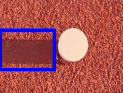


Spatially Varying Regions In a spatially varying dataset shown in Fig. 8, the shadow/specular regions of the scenes constantly change, while the diffuse reflectance of the objects in the static scene always remains the same. To help our network focus on the large shadow/specular regions in the spatially varying dataset to remove them, we use feature statistics and the normalization layer to capture the spatial-variant property of shadows/specularities. Since the mean and variance of the features encode the statistics of an image, aligning them implies transferring the style of the image.
Instance Normalization (IN) (Huang and Belongie 2017) is used in unsupervised style transfer (Liu et al. 2020b): , where and are the channel-wise mean and standard deviation, and is the activation of the previous convolutional layer. Unlike IN, layer normalization (LN) (Ba, Kiros, and Hinton 2016) captures the average and variance of each pixel among a batch of input data: , where and are the layer-wise mean and the standard deviation. Our S-Aware network dynamically adjusts the ratio between IN and LN operations: , where and are parameters generated by the fully connected layer. , are the channel-wise, layer-wise normalization functions, respectively.
Adversarial and Translation Losses Our S-Aware network, , is coupled with a discriminator . We use the least-square GAN (LSGAN) adversarial losses to stabilize our network training:
When the S-Aware network, , takes the original input, it outputs the reflectance layer. We enforce the following loss:
| (6) |
Diffuse Loss We learn the reflectance layer also from the diffuse reflection component , where with is the true diffuse reflectance layer. For images suffered only from shadows, the diffuse reflection component is the image itself, where . For images suffered from specular highlights, the diffuse reflection component can be computed: (Shafer 1985; Tan and Ikeuchi 2005), where is the specular reflection component. Some real (Yi, Tan, and Lin 2020) and synthetic datasets (Shi et al. 2017) provide the information of the diffuse reflection component and the corresponding image together, which can be used in our training. Hence, we define our diffuse loss as:
| (7) |
Overall Loss We multiply each loss function with its respective weight, and sum them together to obtain our overall loss function. The weights of the losses, , , are empirically set to 5, 1, 5 in our experiments. The weights of are 1, since they are in the same scale.


| Methods | Training set | WHDR% |
| STAR (Xu et al. 2020) | ||
| IIW (Bell, Bala, and Snavely 2014) | ||
| ShapeNet (Shi et al. 2017) | ShapeNet (2.5M) | |
| IntrinsicNet (Baslamisli, Le, and Gevers 2018) | ShapeNet (20K) | |
| CGI (Li and Snavely 2018a) | SUNCG | |
| InvRen (Yu and Smith 2019) | MegaDepth | |
| PIE-Net (Das, Karaoglu, and Gevers 2022) | NED+IIW | |
| Fan et al. (Fan et al. 2018)*11 1 | IIW | 14.45 |
| Yi (Yi, Tan, and Lin 2020) | CustomerPhotos | |
| Physics (Baslamisli et al. 2021b) | ShapeNet (20K) | |
| Ma et al. (Ma et al. 2018) | IIW | |
| IIDWW (Li and Snavely 2018b) | BigTime | |
| USI3D (Liu et al. 2020b) | CGI+IIW | |
| UIDNet (Zhang et al. 2021) | ||
| Ours | IIW | 17.97 |
Experimental Results
Reflectance Layer Estimation on Shadows To evaluate our method, we use 2 real (MIT Intrinsic, IIW) and 2 synthetic intrinsic image decomposition datasets (MPI-Sintel, ShapeNet), and 2 shadow datasets (SRD, USR). Fig. 9 and Fig. 10 show our results on the real image USR shadow (Hu et al. 2019) and MIT Intrinsic dataset (Grosse et al. 2009). Fig. 12 shows our results on the synthetic datasets MPI-Sintel (Butler et al. 2012) and ShapeNet (Chang et al. 2015). Most SOTA methods perform poorly in separating shadows from the reflectance layer. When the images have shadow regions, these methods cannot estimate the information under the shadow regions. Our results are free from shadows.
We make a fair comparison with SOTA intrinsic image decomposition methods: PIENet (Das, Karaoglu, and Gevers 2022), UIDNet (Zhang et al. 2021), ShadingNet (Baslamisli et al. 2021a), Physics (Baslamisli et al. 2021b), USI3D (Liu et al. 2020b); optimization-based method: STAR (Xu et al. 2020), inverse rendering method: InverseRenNet (Yu and Smith 2019), etc.
Reflectance Layer Estimation on Specularities To evaluate our method, we use 1 synthetic intrinsic image decomposition dataset and 1 real specular dataset. Fig. 11 shows our results on real (Yi, Tan, and Lin 2020) and synthetic specular ShapeNet (Shi et al. 2017) datasets. Our method estimates the reflectance layer more effectively, in particular for the specular regions, while others may fail to recover some parts of the specular regions, leaving black artefacts in the specular/saturated regions.
To fairly compare to specular methods, we include learning-based intrinsic image decomposition methods: Yi (Yi, Tan, and Lin 2020), ShapeNet (Shi et al. 2017), inverse rendering method: Li (Li et al. 2020), etc. We also include learning-based highlight separation method (Fu et al. 2021), optimization-based methods (Guo, Zhou, and Wang 2018; Shen and Zheng 2013; Yang, Wang, and Ahuja 2010; Tan and Ikeuchi 2005).




Quantitative Evaluation Tables 1, 2 show quantitative results on IIW and ShapeNet datasets. In Table 1, for the quantitative evaluation of reflectance images, we employ the weighted human disagreement rate (WHDR) from (Bell, Bala, and Snavely 2014). In Table 2, we employ si-MSE, si-LMSE from (Barron and Malik 2014).
Ablation Studies We conduct ablation studies to analyze the effectiveness of our first-stage reflectance layer guidance, which is shown in Fig. 13. To show the effectiveness of the first stage, we train our network without the first stage. We directly input the image to the second stage, bypassing the first stage. Table 2 shows that our first stage has a performance gain of 35% (from 0.85 to 0.63) on the ShapeNet dataset; implying our first stage provides a good initial shadow/specular-free guidance. For the first stage, we further study the effectiveness of shadow-free loss () and specular-free loss (). We use shadow/specular-free images in our losses to constrain our initial estimate. We also use other losses to constrain our initial estimate. Hence, the output of our first stage can outperform specular/shadow-free images. For the second stage, we compare our results with and without S-Aware design. That means we remove the S-Classifier and the classification loss. The corresponding quantitative results are shown in Table 2.
| si-MSE | si-LMSE | |||
| Methods | R | S | Avg. | Total |
| LM (Li and Brown 2014) | 3.38 | 2.96 | 3.17 | 6.23 |
| Fan et al. (Fan et al. 2018) | 3.02 | 3.15 | 3.09 | 7.17 |
| Ma et al. (Ma et al. 2018) | 2.84 | 2.62 | 2.73 | 5.44 |
| USI3D (Liu et al. 2020b) | 1.85 | 1.08 | 1.47 | 4.65 |
| Ours w/o stage2 | 1.13 | 2.00 | 1.57 | 4.93 |
| Ours w/o stage1 | 0.85 | 2.17 | 1.51 | 4.85 |
| Ours w/o S-Aware | 0.79 | 2.05 | 1.42 | 4.15 |
| Ours w/o | 0.73 | 2.07 | 1.40 | 4.73 |
| Ours w/o | 0.66 | 2.04 | 1.35 | 4.19 |
| Ours | 0.63 | 2.00 | 1.31 | 4.14 |


Conclusion
In this paper, we have proposed a two-stage network to estimate the reflectance layer free from shadows and specularities. With the reflectance guidance and the S-Aware network, our method can robustly separate shadows and specularities out of the reflectance layer. We propose novel shadow-free and specular-free losses to estimate the initial reflectance layer. To further refine the reflectance layer, we integrate a classifier into our network, enabling our method to focus on shadow/specular regions. Experimental results have confirmed that our method is effective and outperforms the state-of-the-art reflectance layer estimation methods.
Acknowledgements
This research/project is supported by the National Research Foundation, Singapore under its AI Singapore Programme (AISG Award No: AISG2-PhD/2022-01-037[T]), and partially supported by MOE2019-T2-1-130. Robby T. Tan’s work is supported by MOE2019-T2-1-130. This research work is also partially supported by the Basic and Frontier Research Project of PCL and the Major Key Project of PCL.
References
- Ba, Kiros, and Hinton (2016) Ba, J. L.; Kiros, J. R.; and Hinton, G. E. 2016. Layer normalization. arXiv preprint arXiv:1607.06450.
- Barron and Malik (2014) Barron, J. T.; and Malik, J. 2014. Shape, illumination, and reflectance from shading. IEEE transactions on pattern analysis and machine intelligence, 37(8): 1670–1687.
- Barrow et al. (1978) Barrow, H.; Tenenbaum, J.; Hanson, A.; and Riseman, E. 1978. Recovering intrinsic scene characteristics. Comput. Vis. Syst, 2(3-26): 2.
- Baslamisli et al. (2021a) Baslamisli, A. S.; Das, P.; Le, H.-A.; Karaoglu, S.; and Gevers, T. 2021a. ShadingNet: image intrinsics by fine-grained shading decomposition. International Journal of Computer Vision, 1–29.
- Baslamisli, Le, and Gevers (2018) Baslamisli, A. S.; Le, H.-A.; and Gevers, T. 2018. CNN based learning using reflection and retinex models for intrinsic image decomposition. In Proceedings of the IEEE Conference on Computer Vision and Pattern Recognition, 6674–6683.
- Baslamisli et al. (2021b) Baslamisli, A. S.; Liu, Y.; Karaoglu, S.; and Gevers, T. 2021b. Physics-based shading reconstruction for intrinsic image decomposition. Computer Vision and Image Understanding, 205: 103183.
- Bell, Bala, and Snavely (2014) Bell, S.; Bala, K.; and Snavely, N. 2014. Intrinsic images in the wild. ACM Transactions on Graphics (TOG), 33(4): 1–12.
- Bi, Han, and Yu (2015) Bi, S.; Han, X.; and Yu, Y. 2015. An l 1 image transform for edge-preserving smoothing and scene-level intrinsic decomposition. ACM Transactions on Graphics (TOG), 34(4): 1–12.
- Bonneel et al. (2014) Bonneel, N.; Sunkavalli, K.; Tompkin, J.; Sun, D.; Paris, S.; and Pfister, H. 2014. Interactive intrinsic video editing. ACM Transactions on Graphics (TOG), 33(6): 1–10.
- Butler et al. (2012) Butler, D. J.; Wulff, J.; Stanley, G. B.; and Black, M. J. 2012. A naturalistic open source movie for optical flow evaluation. In European conference on computer vision, 611–625. Springer.
- Chang et al. (2015) Chang, A. X.; Funkhouser, T.; Guibas, L.; Hanrahan, P.; Huang, Q.; Li, Z.; Savarese, S.; Savva, M.; Song, S.; Su, H.; et al. 2015. Shapenet: An information-rich 3d model repository. arXiv preprint arXiv:1512.03012.
- Das, Karaoglu, and Gevers (2022) Das, P.; Karaoglu, S.; and Gevers, T. 2022. PIE-Net: Photometric Invariant Edge Guided Network for Intrinsic Image Decomposition. In Proceedings of the IEEE/CVF Conference on Computer Vision and Pattern Recognition, 19790–19799.
- Drew, Finlayson, and Hordley (2003) Drew, M. S.; Finlayson, G. D.; and Hordley, S. D. 2003. Recovery of chromaticity image free from shadows via illumination invariance. In IEEE Workshop on Color and Photometric Methods in Computer Vision, ICCV’03, 32–39. Citeseer.
- Emmanuel J. Candès (2008) Emmanuel J. Candès, S. P. B., Michael B. Wakin. 2008. Enhancing Sparsity by Reweighted Minimization. Journal of Fourier Analysis and Applications, 14: 877–905.
- Fan et al. (2018) Fan, Q.; Yang, J.; Hua, G.; Chen, B.; and Wipf, D. 2018. Revisiting deep intrinsic image decompositions. In Proceedings of the IEEE conference on computer vision and pattern recognition, 8944–8952.
- Finlayson, Drew, and Lu (2004) Finlayson, G. D.; Drew, M. S.; and Lu, C. 2004. Intrinsic images by entropy minimization. In European conference on computer vision, 582–595.
- Finlayson, Drew, and Lu (2009) Finlayson, G. D.; Drew, M. S.; and Lu, C. 2009. Entropy minimization for shadow removal. International Journal of Computer Vision, 85(1): 35–57.
- Fu et al. (2021) Fu, G.; Zhang, Q.; Zhu, L.; Li, P.; and Xiao, C. 2021. A multi-task network for joint specular highlight detection and removal. In Proceedings of the IEEE/CVF Conference on Computer Vision and Pattern Recognition, 7752–7761.
- Garces et al. (2012) Garces, E.; Munoz, A.; Lopez-Moreno, J.; and Gutierrez, D. 2012. Intrinsic images by clustering. In Computer graphics forum, volume 31, 1415–1424. Wiley Online Library.
- Garces et al. (2022) Garces, E.; Rodriguez-Pardo, C.; Casas, D.; and Lopez-Moreno, J. 2022. A Survey on Intrinsic Images: Delving Deep into Lambert and Beyond. International Journal of Computer Vision, 130(3): 836–868.
- Grosse et al. (2009) Grosse, R.; Johnson, M. K.; Adelson, E. H.; and Freeman, W. T. 2009. Ground truth dataset and baseline evaluations for intrinsic image algorithms. In 2009 IEEE 12th International Conference on Computer Vision, 2335–2342. IEEE.
- Guo, Zhou, and Wang (2018) Guo, J.; Zhou, Z.; and Wang, L. 2018. Single image highlight removal with a sparse and low-rank reflection model. In Proceedings of the European Conference on Computer Vision (ECCV), 268–283.
- Guo et al. (2023) Guo, L.; Huang, S.; Liu, D.; Cheng, H.; and Wen, B. 2023. ShadowFormer: Global Context Helps Image Shadow Removal. arXiv preprint arXiv:2302.01650.
- Han et al. (2022) Han, J.; Li, W.; Fang, P.; Sun, C.; Hong, J.; Armin, M. A.; Petersson, L.; and Li, H. 2022. Blind image decomposition. In Computer Vision–ECCV 2022: 17th European Conference, Tel Aviv, Israel, October 23–27, 2022, Proceedings, Part XVIII, 218–237. Springer.
- Hu et al. (2019) Hu, X.; Jiang, Y.; Fu, C.-W.; and Heng, P.-A. 2019. Mask-ShadowGAN: Learning to remove shadows from unpaired data. In Proceedings of the IEEE/CVF International Conference on Computer Vision, 2472–2481.
- Huang and Belongie (2017) Huang, X.; and Belongie, S. 2017. Arbitrary Style Transfer in Real-Time With Adaptive Instance Normalization. In Proceedings of the IEEE International Conference on Computer Vision (ICCV).
- Jin, Sharma, and Tan (2021) Jin, Y.; Sharma, A.; and Tan, R. T. 2021. DC-ShadowNet: Single-Image Hard and Soft Shadow Removal Using Unsupervised Domain-Classifier Guided Network. In Proceedings of the IEEE/CVF International Conference on Computer Vision, 5027–5036.
- Jin et al. (2022a) Jin, Y.; Yan, W.; Yang, W.; and Tan, R. T. 2022a. Structure Representation Network and Uncertainty Feedback Learning for Dense Non-Uniform Fog Removal. In Proceedings of the Asian Conference on Computer Vision, 2041–2058.
- Jin, Yang, and Tan (2022) Jin, Y.; Yang, W.; and Tan, R. T. 2022. Unsupervised night image enhancement: When layer decomposition meets light-effects suppression. In European Conference on Computer Vision, 404–421. Springer.
- Jin et al. (2022b) Jin, Y.; Yang, W.; Ye, W.; Yuan, Y.; and Tan, R. T. 2022b. ShadowDiffusion: Diffusion-based Shadow Removal using Classifier-driven Attention and Structure Preservation. arXiv preprint arXiv:2211.08089.
- Kawakami, Ikeuchi, and Tan (2005) Kawakami, R.; Ikeuchi, K.; and Tan, R. T. 2005. Consistent surface color for texturing large objects in outdoor scenes. In Tenth IEEE International Conference on Computer Vision (ICCV’05) Volume 1, volume 2, 1200–1207. IEEE.
- Kim et al. (2019) Kim, J.; Kim, M.; Kang, H.; and Lee, K. 2019. U-GAT-IT: unsupervised generative attentional networks with adaptive layer-instance normalization for image-to-image translation. arXiv preprint arXiv:1907.10830.
- Kovacs et al. (2017) Kovacs, B.; Bell, S.; Snavely, N.; and Bala, K. 2017. Shading annotations in the wild. In Proceedings of the IEEE Conference on Computer Vision and Pattern Recognition, 6998–7007.
- Land and McCann (1971) Land, E. H.; and McCann, J. J. 1971. Lightness and retinex theory. Josa, 61(1): 1–11.
- Lettry, Vanhoey, and Van Gool (2018) Lettry, L.; Vanhoey, K.; and Van Gool, L. 2018. Unsupervised deep single-image intrinsic decomposition using illumination-varying image sequences. In Computer Graphics Forum, volume 37, 409–419. Wiley Online Library.
- Li, Tan, and Cheong (2018) Li, R.; Tan, R. T.; and Cheong, L.-F. 2018. Robust optical flow in rainy scenes. In Proceedings of the European Conference on Computer Vision (ECCV), 288–304.
- Li and Brown (2014) Li, Y.; and Brown, M. S. 2014. Single image layer separation using relative smoothness. In Proceedings of the IEEE Conference on Computer Vision and Pattern Recognition, 2752–2759.
- Li et al. (2020) Li, Z.; Shafiei, M.; Ramamoorthi, R.; Sunkavalli, K.; and Chandraker, M. 2020. Inverse rendering for complex indoor scenes: Shape, spatially-varying lighting and svbrdf from a single image. In Proceedings of the IEEE/CVF Conference on Computer Vision and Pattern Recognition, 2475–2484.
- Li and Snavely (2018a) Li, Z.; and Snavely, N. 2018a. Cgintrinsics: Better intrinsic image decomposition through physically-based rendering. In Proceedings of the European Conference on Computer Vision (ECCV), 371–387.
- Li and Snavely (2018b) Li, Z.; and Snavely, N. 2018b. Learning intrinsic image decomposition from watching the world. In Proceedings of the IEEE Conference on Computer Vision and Pattern Recognition, 9039–9048.
- Liu et al. (2020a) Liu, A.; Ginosar, S.; Zhou, T.; Efros, A. A.; and Snavely, N. 2020a. Learning to factorize and relight a city. In Computer Vision–ECCV 2020: 16th European Conference, Glasgow, UK, August 23–28, 2020, Proceedings, Part IV 16, 544–561. Springer.
- Liu et al. (2020b) Liu, Y.; Li, Y.; You, S.; and Lu, F. 2020b. Unsupervised learning for intrinsic image decomposition from a single image. In Proceedings of the IEEE/CVF Conference on Computer Vision and Pattern Recognition, 3248–3257.
- Ma et al. (2018) Ma, W.-C.; Chu, H.; Zhou, B.; Urtasun, R.; and Torralba, A. 2018. Single image intrinsic decomposition without a single intrinsic image. In Proceedings of the European Conference on Computer Vision (ECCV), 201–217.
- Narihira, Maire, and Yu (2015) Narihira, T.; Maire, M.; and Yu, S. X. 2015. Direct intrinsics: Learning albedo-shading decomposition by convolutional regression. In Proceedings of the IEEE international conference on computer vision, 2992–2992.
- Qu et al. (2017) Qu, L.; Tian, J.; He, S.; Tang, Y.; and Lau, R. W. 2017. Deshadownet: A multi-context embedding deep network for shadow removal. In Proceedings of the IEEE Conference on Computer Vision and Pattern Recognition, 4067–4075.
- Shafer (1985) Shafer, S. A. 1985. Using color to separate reflection components. Color Research & Application, 10(4): 210–218.
- Shen and Zheng (2013) Shen, H.-L.; and Zheng, Z.-H. 2013. Real-time highlight removal using intensity ratio. Applied optics, 52(19): 4483–4493.
- Shi et al. (2017) Shi, J.; Dong, Y.; Su, H.; and Yu, S. X. 2017. Learning non-lambertian object intrinsics across shapenet categories. In Proceedings of the IEEE Conference on Computer Vision and Pattern Recognition, 1685–1694.
- Tan (2021) Tan, R. T. 2021. Specularity, specular reflectance. In Computer Vision: A Reference Guide, 1185–1188. Springer.
- Tan and Ikeuchi (2005) Tan, R. T.; and Ikeuchi, K. 2005. Separating Reflection Components of Textured Surfaces Using a Single Image. IEEE Trans. Pattern Anal. Mach. Intell., 27(2): 178–193.
- Tan, Nishino, and Ikeuchi (2003) Tan, T.; Nishino, K.; and Ikeuchi, K. 2003. Illumination chromaticity estimation using inverse-intensity chromaticity space. In 2003 IEEE Computer Society Conference on Computer Vision and Pattern Recognition, 2003. Proceedings., volume 1, I–I. IEEE.
- Wang, Li, and Yang (2018) Wang, J.; Li, X.; and Yang, J. 2018. Stacked conditional generative adversarial networks for jointly learning shadow detection and shadow removal. In Proceedings of the IEEE Conference on Computer Vision and Pattern Recognition, 1788–1797.
- Xu et al. (2020) Xu, J.; Hou, Y.; Ren, D.; Liu, L.; Zhu, F.; Yu, M.; Wang, H.; and Shao, L. 2020. Star: A structure and texture aware retinex model. IEEE Transactions on Image Processing, 29: 5022–5037.
- Yang, Wang, and Ahuja (2010) Yang, Q.; Wang, S.; and Ahuja, N. 2010. Real-time specular highlight removal using bilateral filtering. In European conference on computer vision, 87–100. Springer.
- Yi, Tan, and Lin (2020) Yi, R.; Tan, P.; and Lin, S. 2020. Leveraging Multi-View Image Sets for Unsupervised Intrinsic Image Decomposition and Highlight Separation. In Proceedings of the AAAI Conference on Artificial Intelligence, volume 34, 12685–12692.
- Yu and Smith (2019) Yu, Y.; and Smith, W. A. 2019. InverseRenderNet: Learning single image inverse rendering. In Proceedings of the IEEE/CVF Conference on Computer Vision and Pattern Recognition, 3155–3164.
- Zhang et al. (2021) Zhang, Q.; Zhou, J.; Zhu, L.; Sun, W.; Xiao, C.; and Zheng, W.-S. 2021. Unsupervised Intrinsic Image Decomposition using Internal Self-similarity Cues. IEEE Transactions on Pattern Analysis and Machine Intelligence.
- Zhang, Ng, and Chen (2018) Zhang, X.; Ng, R.; and Chen, Q. 2018. Single image reflection separation with perceptual losses. In Proceedings of the IEEE conference on computer vision and pattern recognition, 4786–4794.
- Zhou et al. (2016) Zhou, B.; Khosla, A.; Lapedriza, A.; Oliva, A.; and Torralba, A. 2016. Learning deep features for discriminative localization. In Proceedings of the IEEE conference on computer vision and pattern recognition, 2921–2929.