The gerrymander sequence, or A348456.

The gerrymander sequence, $g_{L}$, counts the number of ways to dissect a $2L\times 2L$ chessboard into two polyominoes, each of area $2L^{2}.$ Until very recently only the first three terms of this sequence were known. Following a challenge from Neil Sloane the sequence was extended by Kauers, Koutschan and Spahn from 3 terms to 7 terms [1]. In this paper (among other calculations) we further extend the gerrymander sequence to 11 terms.

Our approach is slightly more general. Divide an $L\times L$ square into two connected regions but not necessarily of equal area. We refer to these as generalised gerrymander configurations. Let $g_{L,k}$ be the number of such configurations with one region having area $k$ (the other having area $L^{2}-k$). Note that any configuration is counted twice, once for the region of area $k$ and once for the region of area $L^{2}-k$. Then, clearly $g_{L,k}$ is symmetric, so that $g_{L,k}=g_{L,L^{2}-k}.$

Set $i=\lfloor L^{2}/2\rfloor.$ We then define the generalised gerrymander sequence as $\widehat{g}_{L}=g_{L,i}$. For $L$ even $\widehat{g}_{L}$ is twice the gerrymander sequence coefficient, while for $L$ odd, it is one of the two (equal) terms on either side of the half area mark. The sequence $g_{L,k}$ is by definition symmetric and by observation unimodal so $\widehat{g}_{L}$ is the largest term in the sequence¹¹ 1 We cannot prove unimodality, which is not surprising, as it took 150 years to prove unimodality [2] for the much simpler subset of generalised gerrymander configurations in which only steps to the north and east are taken. The area under such a path is given by the $q$-binomial coefficients..

It should be noted that in any generalised gerrymander configuration one (or both) regions has to be a self-avoiding polygon (SAP). This is the key to our efficient enumeration of gerrymanders.

In Figure 1 we display examples of the four distinct cases one has to consider, noting that the grey region is a SAP. Given the constraint of only two connected regions, it follows that the grey region can be chosen so that it contains either zero, one, or two corners of the square.

If the grey region contains none of the corners then it is either a SAP not touching any of the sides or it is a SAP touching one and only one side of the square. In the first case, shown in panel 4 of Figure 1, all cells on the border belongs to the white region. In the second case the part of the SAP along the side must consist of contiguous cells as illustrated in panel 3 of Figure 1. All cells on the remaining sides of the square belongs to the white region.

If the grey region contains one corner then the cells along the two sides next to this corner must be contiguous as shown in panel 2 of Figure 1. All cells along the two remaining sides (top row and right-most column in our example) belongs to the white region. Finally when the grey region contains two corners these must lie on the same side of the square (see panel 1 of Figure 1). All cells on the remaining side (top row in our example) belong to the white region.

By symmetry, configurations shown in panel 1 must be counted twice since the SAP could include the bottom or left side of the square, those in panels 2 and 3 must be counted four times and those in panel 4 must be counted only once. To count generalised gerrymander configurations we therefore need to count SAPs by area (with some constraints which we will detail further in Section 3).

We define an area generating function (or gerrymander polynomial)

$G_{L}(q)$ counts all generalised gerrymander configurations and is a symmetric polynomial. $G_{L}(1)/2$ is the number of ways to partition the square into two connected regions. We calculated $G_{L}(q)$ up to $L=22$, and we extended this up to $L=26$ for the special case of $G_{L}(1)/2$. The first 6 terms of $G_{L}(1)/2$ were obtained by RH Hardin and extended to 14 terms by A Howroyd, see OEIS sequence A068416.

A $n$-step self-avoiding walk (SAW) ${\bf\omega}$ on a regular lattice is a sequence of distinct vertices, $\omega_{0},\omega_{1},\ldots,\omega_{n}$, such that each vertex is a nearest neighbour of its predecessor. SAWs are considered distinct up to translations of the starting point $\omega_{0}$. If $\omega_{0}$ and $\omega_{n}$ are nearest-neighbours we can form a closed $(n+1)$-step self-avoiding polygon (SAP) by adding an edge between the two end-points.

We recently studied SAWs on an $L\times L$ square lattice, with the walks starting at the south-west corner $(0,0)$ and finishing at the north-east corner $(L,L),$ and constrained within the square (see the first diagram in Figure 2), and refer to these as WCAS [3]. Consider the generating function $C_{L}(x)=\sum_{n}c_{L,n}x^{n},$ where $c_{L,n}$ denotes the number of WCAS of length $n$ on a $L\times L$ square.

The existence of the limit

was proved in both [4] and [5] by different methods, and has recently been given a third proof [6]. In our recent work [3] we estimated $\lambda=1.7445498\pm 0.0000012.$ We also estimated the sub-dominant terms by finding compelling numerical evidence for the asymptotic behaviour

where $b=-0.04354\pm 0.0001,$ $c=0.5624\pm 0.0005,$ and $g=0.000\pm 0.005,$ from which we conjectured that $g=0$, exactly. This conjectured asymptotic form has received support by a very recent result of Whittington [6] who has proved that $C_{L}(1)=\lambda^{L^{2}+O(L)},$ a significant improvement on the previous result $C_{L}(1)=\lambda^{L^{2}+o(L^{2})}.$

For SAPs crossing a square (PCAS) our analysis clearly demonstrated that the growth constant is the same as for WCAS. We prove this result in Section 2. We also conjectured that the subdominant term $\lambda^{b}$ is the same as for WCAS, estimated $c\approx-1.197,$ and that the corresponding exponent $g=-\frac{1}{2}.$

In Section 2 we prove that the growth constant for the generalised gerrymander sequence equals the growth constant for WCAS. We use the data generated in this study to estimate the sub-dominant behaviour, and find that $\widehat{g}_{L}\sim\lambda^{L^{2}+dL+e}\cdot L^{h},$ where $d=-4.04354\pm 0.0001,$ $e\approx 8$ and $h=0.75\pm 0.01$ for generalised gerrymanders, and is likely $3/4$ exactly. Consequently we find that the coefficients of the gerrymander sequence $g_{L}$ (OEIS A348456) grow as $g_{L}\sim\lambda^{4L^{2}+2dL+e}\cdot(2L)^{h}$.

Finally, we find $G_{L}(1)/2\sim\lambda^{L^{2}+dL+e}\cdot L^{g},$ where now $d=-4.04354\pm 0.0001,$ $e\approx 8$ and $g=1.75\pm 0.01,$ and is likely $7/4$ exactly. So this is just $L$ times the corresponding coefficient $\widehat{g}_{L}.$

In Section 2 we present proofs that the growth constants for both PCAS and gerrymanders are equal to the growth constant for WCAS. In Section 3 we give a description of the new and very efficient algorithm we used to calculate the series for generalised gerrymanders. Section 5 contains an analysis of the generalised gerrymander sequence. Section 6 contains our conclusions and gives a summary of the estimates we have obtained.

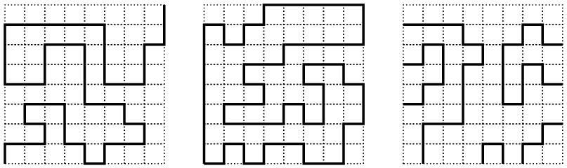
In Figure 2 we show, from left to right, a WCAS, a PCAS, and a cow-patch, so called as if we colour each domain within the figure alternately black and white, the resulting figure resembles the pattern on the skin of a suitably endowed cow. In [7] it was proved that WCAS and cow-patches have the same growth constant. We next give a proof that PCAS and WCAS have the same growth constant.

In Section 1 we argued that gerrymander configurations (partitioning the square into two connected regions) can be enumerated by considering the grey SAPs shown in Figure 1.

The SAPs in panels 1 and 2 can be counted in a single calculation for each $L$ and require counting SAPs in rectangles of size $(L-1)\times L$ with the constraint that the SAP has a single column of cells starting from the bottom of the rectangle and with the further constraint that once the SAP leaves the bottom it can never return.

The SAPs in panel 3 are SAPs in a rectangle of size $(L-2)\times(L-1)$ with the constraint that there is a single column of cells on the left boundary. Finally, the configurations in panel 4 are unconstrained SAPs in an $(L-2)\times(L-2)$ square. These two cases can also be counted in a single calculation as shown later.

To calculate the (generalised) gerrymander sequence we need to count the configurations where each region has equal (or close to) area. To achieve this we actually calculate the complete gerrymander polynomials $G_{L}(q)$ by enumerating the grey SAPs of Figure 1 by area. When combining the counts for the four SAP cases, with appropriate symmetry factors, we get the coefficients $p_{L,k}$, which count the contributions to $G(q)$ from grey SAPs of area $k$ in a $L\times L$ square. We then use the coefficients $p_{L,k}$ to calculate $G_{L}(q)$ since $g_{L,k}=p_{L,k}+p_{L,L^{2}-k}$, where $p_{L,L^{2}-k}$ accounts for the contributions from white regions of area $k$.

In Figure 6 we explicitly list all the configurations we must consider to calculate $G_{3}(q)$. The top row shows the contributions from configurations of panel 1 in Figure 1, the middle row arises from configurations of panel 2 while the last row arises from configurations in panels 3 and 4. The contributions to $G_{3}(q)$ are listed below each panel and the first term comes from the grey region while the second term is from the white region. Counting only the contributions from the grey regions (as done by our algorithms) gives rise to the polynomial, $9q+12q^{2}+14q^{3}+10q^{4}+6q^{5}+2q^{6}$, which has coefficients $p_{3,k}$. From these we can then calculate the corresponding gerrymander polynomial,

We implemented the very efficient transfer matrix (TM) algorithm of Iwashita et al. [9] for enumerating SAPs on the square lattice making use of a minimal perfect hash function and in-place memory updating of the arrays for the counts of the number of SAPs. We gave a quite detailed description of the algorithm applied to paths on the hexagonal lattice in our recent paper [3] and most of the considerations from that paper apply to the case of SAPs on the square lattice. So here we will just give a brief description of the main points of the algorithm and point our readers to [3] for further details.

If we draw a line across the square as shown in Figure 7 we observe that the partial SAP to the left of the intersection consists of arcs connecting two edges on the intersection and a ‘special’ vertex where there is a kink in the intersection. On two-dimensional lattices arcs cannot intertwine so each arc end can be assigned a label depending on whether it is the lower or upper end of an arc, and these labels will form a balanced parenthesis. The vertex at the kink in the intersection can have an additional blocked state if two edges of the partial SAP are incident on the vertex (as shown in the figure). We shall refer to the configuration along the intersection as a signature, denoted by $\Sigma$, which can be represented by a string of states, $\sigma_{i}$, where

For each signature $\Sigma$ we simply count the number of partial SAPs, ${\mathcal{C}}(\raisebox{-1.50696pt}{{\large$\Sigma$}},q)$, where ${\mathcal{C}}(\raisebox{-1.50696pt}{{\large$\Sigma$}},q)$ is a polynomial in $q$ such that the coefficient $p_{k}$ of $q^{k}$ equals the number of partial SAPs of area $k$. SAPs are counted by moving the intersection so as to add a single cell and two edges at a time, as illustrated in Figure 7. For each column of height $W$ the TM move from the left panel of Figure 7 is used $W-1$ times followed by the final move shown in the right panel which completes a column. This sequence of moves is then repeated to construct a rectangle of the required length.

The updating of the counting polynomial ${\mathcal{C}}(\raisebox{-1.50696pt}{{\large$\Sigma$}},q)$ depends on the states of the bottom edge to the left of the new cell and the topmost vertex of the new cell. The new cell can either belong to a completed SAP or not and it will belong to a SAP if there is an odd number of occupied edge states below the new cell.

In Figure 8 we display the possible local ‘input’ states and the ‘output’ states which arise as the kink in the boundary is propagated by one step (we left out a panel identical to the second panel from the top but involving an upper arc end rather than a lower arc end). We shall refer to the signature before the move as the source, $\raisebox{-1.50696pt}{{\large$\Sigma$}}_{\rm S}$, and a signature produced as a result of the move as a target, $\raisebox{-1.50696pt}{{\large$\Sigma$}}_{\rm T}$.

It is possible to represent the signatures as Motzkin paths, which are directed walks from $(0,0)$ to $(n,0)$ in the first quadrant of the square lattice with step-set $\Omega=\{(1,0),(1,1),(1,-1)\}$. The basic mapping from a signature to a Motzkin path is to map to horizontal steps, to up steps, and to down steps. Let ${\mathcal{M}}_{n}$ be the set of $n$-step Motzkin paths. Consider enumerations on a rectangle of size $W\times L$ ($W\leq L)$. The set of unblocked signatures is given by the set ${\mathcal{M}}_{W+1}$ since there are $W$ edges and one vertex along the TM intersection. A signature can have only a single blocked vertex whose position (in either the source or the target signature) is given by the position of the kink in the TM intersection and the remaining states form a Motzkin path of length $W$. The set of blocked signatures can therefore be represented by the set ${\mathcal{M}}_{W}$.

Using the mapping of signatures to Motzkin paths one can construct minimal perfect hash functions $\Phi:{\mathcal{M}}_{W+1}\to\{1,\ldots,|{\mathcal{M}}_{W+1}|\}$ for unblocked signatures and $\Psi:{\mathcal{M}}_{W}\to\{1,\ldots,|{\mathcal{M}}_{W}|\}$ for blocked signatures as described in [9, 3].

In Algorithms 1 and 2 we give pseudo code for the updates to the counting polynomials ${\mathcal{C}}(\raisebox{-1.50696pt}{{\large$\Sigma$}},q)$. InputState simply extracts the states of the edge and vertex involved in the update. AddArea determines if the cell added in the TM move adds to the area of the SAP. ChangeSignature changes the states of the input states to those indicated by the two blue tiles. RelabelSignature changes the input states to empty states and finds and relabels the matching arc end in those updates where two arc ends are connected in a TM update.

A technical point should be noted. In the update at line 7 of Algorithm 1 there should seemingly be a factor $q^{1-\Delta}$ multiplying the term on the right. After all inserting a new arc changes whether or not the added cell lies within the SAP. The factor is missing at this point because the target signature is processed later as a source and any missing unit of area is added at line 32. One could rearrange the code and include the processing happening for the case when processing the case and then do nothing for the case .

The four cases of SAPs we enumerate can in fact be done in just two separate calculations. This requires some minor changes to the code of Algorithms 1 and 2 and different ways of initializing ${\mathcal{C}}(\raisebox{-1.50696pt}{{\large$\Sigma$}},q)$ to account for the permitted columns on the left-most boundary.

The SAPs in panels 1 and 2 of Figure 1 can be counted in one calculation on a rectangle of size $(L-1)\times L$. Initially, ${\mathcal{C}}(\raisebox{-1.50696pt}{{\large$\Sigma$}},q)=2q^{k}$ for signatures with a at position 0, a at position $k$, and all other states . This gives a column of cells on the left boundary starting from the bottom. Next we add $L-1$ columns to the lattice by the TM updates with the addition to the SAP count done as: ${\mathcal{P}}(q)\leftarrow{\mathcal{P}}(q)+2{\mathcal{C}}[\Phi(\raisebox{-1.50696pt}{{\large$\Sigma$}}_{\rm S}),q]$. Then one adds one extra column, but without adding to the SAP count at case . This ensures that all configurations of panel 2 are counted four times. After the addition of the final column the SAP counts ${\mathcal{P}}(q)$ are updated by adding the counts for the signatures used to initialize ${\mathcal{C}}(\raisebox{-1.50696pt}{{\large$\Sigma$}},q)$, thus counting the configurations in panel 1 twice.

One further change to the algorithm is required. Once a SAP has stepped away from the bottom of the rectangle (there are some empty cells at the bottom of a column) it is not allowed to return to the bottom of the rectangle since this would produce configurations with more than two connected components. This constraint can be easily implemented by some minor changes to Algorithm 2. The insertion of a new arc at line 4 is not permitted so this line is simply removed from the code and the updating at line 12 is changed to, ${\mathcal{C}}[\Phi(\raisebox{-1.50696pt}{{\large$\Sigma$}}_{\rm S}),q]\leftarrow q\big({\mathcal{C}}[\Phi(\raisebox{-1.50696pt}{{\large$\Sigma$}}_{\rm S}),q]+{\mathcal{C}}[\Psi(\raisebox{-1.50696pt}{{\large$\Sigma$}}_{\rm B}),q]\big)$, which prevents the situation where a lower arc end is extended from above to an empty edge on the bottom of the rectangle.

The SAPs in panels 3 and 4 of Figure 1 can be counted in one calculation on a rectangle of size $(L-2)\times(L-1)$. Initially, ${\mathcal{C}}(\raisebox{-1.50696pt}{{\large$\Sigma$}},q)=4q^{k-j}$ for signatures with a at position $j$, a at position $k>j$, and all other states . This gives a column of cells on the left boundary starting at position $j$ and ending at position $k$. Next we add $L-2$ columns by TM updates. This counts configurations in panel 3 four times. The SAPs of panel 4 are just cycles on a $(L-2)\times(L-2)$ square. The counts for these SAPs are added by putting a few extra lines of code after line 32 of Algorithm 1 and line 24 of Algorithm 2:

We used our algorithms to calculate $G_{L}(q)$ up to $L=22$.

Calculating the sequence $G_{L}(1)/2$ is a simplification of the algorithms since we no longer need to keep track of the area of the SAP. That is, the variable $q$ is removed and the count ${\mathcal{C}}(\raisebox{-1.50696pt}{{\large$\Sigma$}})$ is just a number and not a polynomial. This makes the memory use and running time much smaller and we could therefore quite readily extend the counts for $G_{L}(1)/2$ up to $L=26$.

The coefficients become very large and we deal with this by actually performing all calculation modulo various prime numbers and then we reconstruct the actual coefficients using the Chinese remainder theorem. For $G_{L}(q)$ we used primes of the form $p_{i}=2^{30}-r_{i}$ while for $G_{L}(1)/2$ we used primes of the form $p_{i}=2^{62}-r_{i}$, with $r_{i}$ chosen so that we used the largest primes possible.

The algorithms can readily be made parallel using OpenMP for shared memory systems as shown in [3]. The most demanding calculation is $L=22$ for SAPs in panel 1 of Figure 1. The total memory use was just short of 1TB and required 12 primes. The calculations were performed on a system with 2TB of memory and a 48 core 2.6GHz Intel Xeon processor (Icelake). Using all 48 cores each calculation required 3.26 CPU hours per core and had a wall time of 4.04 hours for a fairly respectable 80% CPU utilisation rate.

Similarly for $G_{L}(1)/2$ the most demanding calculation used about 260GB of memory, required 8 primes with each using around 1.66 CPU hours per core with a wall time of 1.92 hours for an 87% CPU utilisation rate.

The enumeration data for all problems studied in this paper and some of the source code used to calculate the exact coefficients can be found at our GitHub repository https://github.com/IwanJensen/Enumerations/tree/Gerrymander.

The sequence $G_{L}(1)/2,$ previously given in the OEIS [10] to 14 terms as sequence A068416 is

In [3] we gave compelling numerical evidence that PCAS behaved as $P_{L}(1)\sim\lambda^{L^{2}+bL+c}\cdot L^{g},$ where $\lambda=1.7445498\pm 0.0000012,$ $b=-0.04354\pm 0.0001,$ $c\approx-1.197$ and $g=-0.500\pm 0.005.$

Having shown that the dominant term for generalised gerrymanders is $\lambda^{L^{2}},$ we make the obvious conjecture that the sub-dominant terms for generalised gerrymanders are similar to those of PCAS, and write $\widehat{g}_{L}\sim\lambda^{L^{2}+dL+e}\cdot L^{h}.$

Then