Meta Architecture for Point Cloud Analysis
Abstract
Recent advances in 3D point cloud analysis bring a diverse set of network architectures to the field. However, the lack of a unified framework to interpret those networks makes any systematic comparison, contrast, or analysis challenging, and practically limits healthy development of the field. In this paper, we take the initiative to explore and propose a unified framework called PointMeta, to which the popular 3D point cloud analysis approaches could fit. This brings three benefits. First, it allows us to compare different approaches in a fair manner, and use quick experiments to verify any empirical observations or assumptions summarized from the comparison. Second, the big picture brought by PointMeta enables us to think across different components, and revisit common beliefs and key design decisions made by the popular approaches. Third, based on the learnings from the previous two analyses, by doing simple tweaks on the existing approaches, we are able to derive a basic building block, termed PointMetaBase. It shows very strong performance in efficiency and effectiveness through extensive experiments on challenging benchmarks, and thus verifies the necessity and benefits of high-level interpretation, contrast, and comparison like PointMeta. In particular, PointMetaBase surpasses the previous state-of-the-art method by 0.7%/1.4/%2.1% mIoU with only 2%/11%/13% of the computation cost on the S3DIS datasets. The code and models are available at https://github.com/linhaojia13/PointMetaBase.
1 Introduction
In the past two decades, the popularity of 3D data acquisition technology has led to great interest in point cloud analysis. Unlike images, point clouds are inherently sparse, unordered, and irregular. These characteristics make it challenging for the powerful convolutional neural networks (CNN) resnet; vgg to extract useful information from point clouds. Early studies attempt to convert the point cloud into grids by either voxelization or 2D projections, such that the standard CNN can be applied, but the applications are limited by the extra computation and information loss.
With the introduction of permutation equivariance and invariance by PointNet pointnet and PointNet++ pointnet2, it is possible to use CNNs to process point clouds in their unstructured format. Following PointNet++ pointnet2, many point-based networks have been introduced, most of which focus on the development of complex building blocks to extract local features, such as the convolution in PointCNN kpconv and the self-attention layer in Point Transformer pointtransformer. Although brought significant performance gains, these models are very complicated. On one hand, this makes the approaches computational demanding and thus limited in applications. On the other hand, it also gives extra challenges in systematic comparison and analysis among the models, and thus impacts efficient development of the field, which ideally would benefit from theoretic and empirical guidance.
The community is well aware of this issue, and research efforts have been put on looking for a unified perspective to compare these methods and identify the most crucial implementation details. PosPool pospool and PointNeXt pointnext take a step toward this goal. Adopting a deep residual architecture as the base network, PosPool pospool evaluates the representative building blocks pointnet2; pointcnn; kpconv; dpc and finds that they perform similarly well. PointNeXt pointnext revisits the improved training and scaling strategies adopted by previous SotA methods deepgcn; kpconv; pointtransformer; assanet and tweaks the early model PointNet++ pointnet2 with the learnings, which achieves state-of-the-art performance. Both of them give insights and inspirations to the community via dedicated experiment designs and extensive empirical analysis. However, neither of them provides a framework that is general enough to fit a broad range of point cloud analysis approaches, such that large scale comparison and contrast could be done.
In this paper, we argue that if viewed from the perspective of basic building blocks, the majority of existing approaches could be fit into a single meta architecture (Sec. 3). We call it PointMeta. PointMeta abstracts the computation pipeline of the building blocks for point cloud analysis into four meta functions: a neighbor update function, a neighbor aggregation function, a point update function and a position embedding function (implicit or explicit). As will be discussed in more details in the next sections, this framework brings three benefits, which are also our core technical contributions:
- •
In the dimension of models, it allows us to compare and contrast different models in a fair manner. So it becomes practical to observe and summarize learnings and assumptions, whose correctness could be further verified through experiments with variables controlled under the same framework. For example, among the systematic analysis on all the components across popular models, we found for the positional embedding function, explicit positional embedding is empirically the best choice (Sec. 4.2).
- •
In the dimension of components, it allows us to have a higher level view across components, and thus to revisit the common beliefs and design decisions of the existing approaches. For example, despite the common perception, we find that the neighbor aggregation blocks may collaborate or compete with the learned neighbor features (Sec. 4.3), and thus should be designed carefully.
- •
Based on the learnings from the previous two dimensions, we are then able to do simple tweaks on the building blocks to apply the best practices (Sec. 4.5). The result building block, PointMetaBase, achieves very strong performance, surpassing the previous state-of-the-art method pointnext by 0.7%/1.4/%2.1% mIoU with only 2%/11%/13% of the computation cost on S3DIS s3dis (Fig. 1), and can act as a baseline for further research.
2 Related Work
Neural Networks for Point Cloud Analysis. The unstructured data format of point cloud makes it difficult to apply CNN directly. To address this challenge, PointNet pointnet introduces permutation equivariance and invariance via point-wise MLP and max pooling, which makes it possible to process point cloud directly. To better capture locality, PointNet++ pointnet2 presents a Set Abstraction module to aggregate features from the neighbor points. Most works after PointNet++ focus on the design of build blocks. Graph-based methods dgcnn; gac; deepgcn utilize graph neural networks to extract local features. Pseudo-grid-based methods pointcnn; tangent; kpconv transform the local features onto pseudo grids which allow for regular convolutions. Adaptive weight-based methods randla; RSNet aggregate the neighbor features via weights adaptively learned from the locality. Recently, Transformer-based block pointtransformer; stratified are introduced to capture local information through self-attention. These proposed building blocks are so complicated that make challenges in systematic comparison and analysis, which suggests an urgent need of a common framework to unify existing models in this field.
3 PointMeta
3.1 Meta Architecture
Inspired by the graph network framework RIBGN, we reformulate existing building blocks for point cloud analysis into a single meta architecture, named PointMeta. As shown in Fig. 2 (a), a PointMeta block is composed of four meta functions: a neighbor update function , a neighbor aggregation function , a point update function and a position embedding function (implicit or explicit). The forward pass of a PointMeta block is as follows:
| (1) |
| (2) |
| (3) |
where and represent the feature and the coordinate of point respectively, and denotes the feature length. Let denote the neighbors of point , and be the feature and coordinate of each neighbor of point respectively, represent all neighbor features of point , represent all neighbor coordinates of point , and denote the neighbor number.
Neighbor update. The first step is to group and update neighbors for each point. Usually, the neighbor features is produced by K-Nearest query as dgcnn; pointtransformer or ball query as pointnet2; assanet; pointnext. The update on neighbor features is usually conducted by a multi-layer perceptions (MLP) to make sure the permutation equivariance of the neighbor update function . Specifically, a permutation transformation on results in the same permutation change on the output of the neighbor update.
Neighbor aggregation. Literally, the neighbor aggregation function is used to aggregate the neighbor features for a center point. Different from , the aggregation function must satisfy permutation invariance, i.e., a permutation transformation on the input will have no influence on the output .
Point update. The point update usually contains an MLP, which is used to further enhance the point features.
Position embedding. Incorporating representations of position information via position embedding is a common practice for Vision Transformer (ViT) rethinkrpe; deit; swin, since ViT models must capture spatial relationships of tokens. We thus introduce the concept of position embedding into PointMeta. Within a point cloud, points are organized in an unstructured format, however the points are highly correlated in the 3D Euclidean space. Therefore, the building block of point cloud analysis should posses the position awareness, which is provided by the position embedding function . The function is usually combined with the neighbor update function or the aggregation function implicitly or explicitly, thus we present them with an bundled notation, or .
One may associate PointMeta with Message Passing Neural Networks (MPNNs) MPNN, which abstracts the calculations on a graph as a message passing process. However, it should be noted that PointMeta has a deeper and more exact abstraction on the neighbor calculations from two aspects compared with applying MPNN directly. First, PointMeta decouples the calculations on neighbor features into a neighbor update and a neighbor aggregation. Second, PointMeta emphasizes the importance of position awareness in the neighbor computation. In contrast, a single message function in MPNN is too rough to describe the calculations on neighbor points. As we will see in the later section, it is easy to use PointMeta to describe and compare the calculation process of the building block of existing models completely and thoroughly, but it is difficult for MPNN.
3.2 Instantiation Examples
In this section, we select three representative models from the literature as the instantiation examples and explain how these models implement the meta functions within PointMeta. We illustrate more instantiation examples dgcnn; pointcnn; randla; pointconv; kpconv; pointnext in the supplementary due to the limited space. Sometimes these meta functions are implemented sophisticatedly, we will decompose them into several subfunctions for the sake of brevity and readability.
PointNet++pointnet2. The neighbor update is described as follows:
where denotes the multi-layer perceptions applied on the concatenated neighbor features. The neighbor aggregation is implemented using a simple max pooling operation,
The point update function is another MLP layer, thus we have
Note that the position embedding function is implicitly implemented by , which incorporates the concatenation of the relative positions and grouping features as input and returns position-aware neighbor features .
Point Transformer pointtransformer. The neighbor update is described as follows:
The neighbor aggregation is implemented using vector self-attention, which is described as
where the denotes the Hadamard product and denotes the vector self-attention (VSA) mask. Finally, the point feature is updated with an MLP layer and a shortcut, then we have
ASSANetassanet. The neighbor update is described as:
where the operation means repeating the features three times to produce . The neighbor aggregation is implemented using an anistropic function, which is described as:
where the position embedding is produced by simply repeating the relative coordinates times. Note that, a similar position embedding and aggregation method are also adopted by PosPool pospool, which is named position pooling. Similar with Point Transformer pointtransformer, the point feature is updated with an MLP layer and a shortcut.
4 Explore Best Practices
Given how many instantiations of PointMeta have appeared in the literature, we should push this general framework as far as possible in the architecture exploration to determine the most crucial implementation details. With the help of PointMeta, it is convenient to use quick experiments with variables controlled to verify any empirical observations or assumptions summarized from the comparison. In this section, we first compare and analyze the building blocks of existing models from the implementation details of these meta functions (Sec. 4.1, 4.2, 4.3, 4.4). Then, we summarize the best practices from the systematic analysis (Sec. 4.5). Finally, applying these practices, we do simple tweaks on the building blocks and propose a simple yet well-performing block, PointMetaBase (Sec. 4.6).
4.1 Neighbor Update
According to the order of Group and MLP operation, the neighbor update function is categorized into two classes:
- •
- •
MLP before Group pointcnn; pospool; assanet; pointtransformer; stratified.
As pointed out by ASSANet assanet, compared with the first order, adopting the second order reduces the FLOPs by times, where denotes the point number, denotes the neighbor number, denotes the layer number of the MLP. Although applying MLP before Group brings a large efficiency gain for the neighbor update, a side effect is that the relative coordinates cannot be used as input for the MLP. However, this problem can be easily solved by other position embedding methods, which is specified in Sec. 4.2.
| Variant |
|
|
| ||||||
|---|---|---|---|---|---|---|---|---|---|
| Plain-Max | 47.3±0.7 | 2.0 | 1.4 | ||||||
| Plain-PP | 65.1±0.2 | 2.0 | 1.5 | ||||||
| Plain-PP-Max | 58.4±0.6 | 2.0 | 1.5 | ||||||
| Plain-IPE-Max | 68.0±0.3 | 2.0 | 13.8 | ||||||
| Plain-EPE-Max | 69.0±0.3 | 2.0 | 1.8 | ||||||
| Plain-EPE-PP | 65.4±0.1 | 2.0 | 1.8 |
4.2 Position Embedding
The manners of implementing the position embedding can be categorized into three classes:
- •
- •
Explicit position embedding (EPE) pointcnn; pointtransformer; stratified.
- •
Implicit position embedding (IPE). Following PointNet++ pointnet2, many methods pointnext; pointmlp; pointweb concatenate the relative coordinates with the neighbor features as inputs of the MLP layer in the neighbor update function. As going deeper through the networks, the dimension of the neighbor features become higher while the coordinates dimension still remains 3. This may cause the loss of position information in the high-level features. In addition, IPE requires applying MLP before Group in the neighbor update function, which will increase the computation times.
Explicit position embedding (EPE). Incorporating explicit representations of position information is a common practice for ViT rethinkrpe; deit; swin. As mentioned in Sec. 3.2, Point Transformer pointtransformer learn a position embedding using and add it to the neighbor features . Compare with IPE, EPE avoid the dimension imbalance between the position representations and the neighbor features. Because the input dimension of is only 3, the computation of EPE become very small by controling the dimension of the hidden layers. PointCNN pointcnn also uses an MLP to implement the EPE function, but it merges the EPE by concatenation instead of addition, which incurs a computation increase. StratifiedFormer stratified maintains a learnable quantized look-up table as EPE. In this section, we select the EPE of Point Transfomer as the representative EPE method for the later experiments due to its simplicity.
Position pooling (PP). As mentioned in Sec. 3.2, ASSANet assanet and PosPool pospool use relative coordinates as weights to pool neighbor features. This way can embed the position information into the neighbor features and make an aggregation function without learnable weights. The efficiency of position pooling is worth affirming, but embedding the position in a non-data-driven way may harm the learned neighbor features.
Empirical analysis. We conduct empirical experiments to evaluate the different PE functions described above. The first step is to construct a plain block as the baseline. Following the suggestion given in Sec. 4.1, the neighbor update function adopts the order of MLP-before-Group. The layer number of the MLP here is set to 1. The neighbor aggregation function is a simple max pooling. The point update function is a 1-layer MLP. We denote this block as Plain-Max. We equip Plain-Max with the three kinds of position embedding described above and compare their performance on Area 5 of S3DIS s3dis. The MLP used respectively in EPE and IPE are both 1-layer. The macro-architecture is in level ”L” (described in Sec. 4.6). As shown in Tab. 1, Plain-EPE-Max achieves the best performance with a tiny computation increase against Plain-PP, Plain-PP-Max and Plain-IPE-Max. Because coupling the neighbor features transformation with position embedding, Plain-IPE incurs heavy redundant computation. In a summary, EPE is the optimal choice among the three kinds of position embeddings.
| Variants |
|
|
| ||||||
|---|---|---|---|---|---|---|---|---|---|
| Point Trans pointtransformer | 70.5±0.3 | 7.8 | 5.6 | ||||||
| Point Trans (-VSA+Max) | 70.3±0.2 | 5.1 | 3.3 |
4.3 Neighbor Aggregation
According to whether learnable weights exist in the neighbor aggregation function, we divide the aggregations function into two types:
- •
- •
Learnable aggregation pointcnn; pointtransformer; stratified; kpconv; pointconv.
Learnable aggregation. As mentioned in Sec. 3.1, the aggregation function should satisfy permutation invariance because the point cloud is unordered. The permutation invariance is acquired by learning a space transformation pointcnn; pointconv, learning pointwise weights pointtransformer, or pairwise self-attention stratified. In this section, we select the vector self-attention of Point Transfomer pointtransformer as the representative implementation of the learnable aggregation function due to its excellent performance.
Non-learnable aggregation. There are two types of non-learnable aggregation in the literatures: position pooling pospool; assanet and max pooling pointnet2; dgcnn; deepgcn; pointnext. As mentioned in Sec. 4.2, position pooling embed the position in a non-data-driven way and may compete with the learned neighbor features. As shown in Tab. 1, Plain-EPE-Max surpasses Plain-EPE-PP significantly, which supports our assumption. Therefore, we select the max pooling as the representive non-learnable aggregation function.
Empirical analysis. We conduct an ablation experiment on Point Transformer pointtransformer to compare the aggregation power of both max pooling and vector self-attention. Specially, we replace the VSA with a max pooling operation (denoted as -VSA+Max). As a result, the aggregation of the ablated Point Transfomer is formulated as:
| (4) |
where . As shown in Tab. 2, compared with VSA, max pooling achieves comparable performance with much fewer parameters and FLOPs. Here comes a question, why max pooling has a comparable power with the learnable aggregation? We explore the answer within our PointMeta framework and find that the max pooling is a special case of VSA but with binary and sparse attention. Specifically, the aggregation function Eq. 4 can be reformulated as follows:
where denotes a softmax function whose temperature approximates 0, which makes the softmax output approximates the binary masks. This formulation reveals the collaboration between max pooling and the neighbor update function, i.e., max pooling is an aggregation function with binary and sparse attention which is generated by applying softmax on the output of the neighbor update
4.4 Point Update
The point update function is used to enhance the point features after the neighbor aggregation. Several existing studies do not implement this function in their building blocks dgcnn; deepgcn, and some other studies use a heavy point update function, such as a 2-layer MLP with an inverted bottleneck stratified; pointnext. A natural question arises: how much computation complexity should we allocate for the point update function? We answer this question via extensive ablated experiments.
Empirical analysis. According to the exploration above, we adopt the Plain-EPE-Max as the baseline due to its excellent performance in the ablated experiments (Tab. 1). Since the computation are concentrated on the MLP of the neighbor update function and point update function, we can allocate computation between the two update functions by changing the configurations of the two MLP. We ablate the MLP from two aspects, i.e., the layer number and whether to use an inverted bottleneck that adopted by PointNeXt pointnext and StratifiedFormer stratified. As shown in Tab. 3, the configuration ”N1P2” can achieve an optimal balance between complexity and performance. More layers or inverted bottlenecks can only promote the model marginally but lead to much more computation.
| Variants |
|
|
| ||||||
|---|---|---|---|---|---|---|---|---|---|
| N1P1 | 69.0±0.3 | 2.0 | 1.7 | ||||||
| N2P0 | 68.7±0.3 | 2.0 | 1.7 | ||||||
| N0P2 | 67.8±0.4 | 2.0 | 1.7 | ||||||
| N1P2 | 69.5±0.3 | 2.7 | 2.0 | ||||||
| N1P2-Inv | 69.7±0.3 | 7.1 | 3.8 | ||||||
| N2P1 | 69.4±0.3 | 2.7 | 2.0 | ||||||
| N2P1-Inv | 69.6±0.4 | 7.1 | 3.8 | ||||||
| N1P3 | 69.5±0.3 | 3.4 | 2.3 | ||||||
| N3P1 | 69.6±0.5 | 3.4 | 2.3 |
4.5 Best Practices
Here we summarize the best practices for the building block as follows:
- •
Postion Embedding. Explicit position embedding can endow the models with better position awareness with a low computation cost comparing with other PE manners.
- •
Point Update. Point update is important and the complexity allocation between the neighbor update and the point update should be properly set.
- •
Neighbor Aggregation. Max pooling is not a pure non-learnable aggregation function, its aggregation power is comparable with the learnable aggregation function but with much less computation complexity. Any exploration for a new aggregation function should set max pooling as the baseline.
- •
Neighbor Update. Applying the MLP before neighbors grouping will bring a times FLOPs reduction comparing with using the contrary order. However, the position embeding function must be carefully chosen for the postition awareness.
The first and the second practice are usually ignored by researchers but are vital for the effectiveness and efficiency of the building block, which is demonstrated in Sec. 4.2 and Sec. 4.4. The third shares a similar viewpoint with PosPool pospool which claims that different local aggregation operators perform similarly. However, from the perspective of PointMeta, we provide a deeper insight that max pooling can be reformulated as a special case of vector self-attention pointtransformer, which makes it have comparable aggregation power comparing with the learnable aggregation function. The fourth practice about neighbor update has been emphasized by ASSANet assanet, we restate it here because it is important to notice its collabration with position embedding function. We believe that these practices can provide a guideline for the future research.
4.6 PointMetaBase
We apply the best practices summarized in Sec. 4.5 to design the building block and implement the four meta functions as simply as possible. We name this block as PointMetaBase, which we hope to become a solid baseline for future research. Fig. 2 (g) shows the architecture of PointMetaBase. The layer number of the first MLP is set to 1 and that of the second MLP is set to 2. The neighbor aggregation function is a simple max pooling. We use the EPE adopted by Point Transformer pointtransformer as the position embedding function. Applying EPE and the MLP-before-Group order, we tweak the set abstraction module pointnet2; pointnext as the reduction block, termed PointMetaSA. We adopt the same scaling strategies and decoder with PointNeXt pointnext to construct our PointMetaBase family:
- •
- •
- •
- •
denotes the channel size of the stem MLP and denotes the number of the PointMetaBase block in each stage. Note that when , only one PointMetaSA block but no PointMetaBase blocks are used at each stage. Due to the excellent efficiency of PointMetaBase, we do not need to construct the network at the level ”B” as done in PointNeXt pointnext. In contrast, we choose to scale the model to a larger level ”XXL”. The full details of network architecture are avaliable in the supplementary materials.
| Method | S3DIS 6-Fold | S3DIS Area-5 | ScanNet mIoU | Params. | FLOPs | Throughput | ||||||||||||||
|
|
|
|
|
|
M | G | (ins./sec.) | ||||||||||||
| PointNet++ pointnet2 | 54.5 | 81.0 | 53.5 | 83.0 | 53.5 | 55.7 | 1.0 | 7.2 | 237 | |||||||||||
| PointCNN pointcnn | 65.4 | 88.1 | 57.3 | 85.9 | - | 45.8 | 0.6 | - | - | |||||||||||
| DeepGCN deepgcn | 60.0 | 85.9 | 52.5 | - | - | - | 3.6 | - | - | |||||||||||
| KPConv kpconv | 70.6 | - | 67.1 | - | 69.2 | 68.6 | 15.0 | - | - | |||||||||||
| RandLA-Net randla | 70.0 | 88.0 | - | - | - | 64.5 | 1.3 | 5.8 | - | |||||||||||
| BAAF-Net baaf | 72.2 | 88.9 | 65.4 | 88.9 | - | - | 5.0 | - | - | |||||||||||
| Point Transformer pointtransformer | 73.5 | 90.2 | 70.4 | 90.8 | 70.6 | - | 7.8 | 5.6 | - | |||||||||||
| CBL cbl | 73.1 | 89.6 | 69.4 | 90.6 | - | 70.5 | 18.6 | - | - | |||||||||||
| ASSANet assanet | - | - | 65.8 | 88.9 | - | - | 2.4 | 2.5 | 300 | |||||||||||
| ASSANet-L assanet | - | - | 68.0 | 89.7 | - | - | 115.6 | 36.2 | 136 | |||||||||||
| PointNeXt-S pointnext | 68.0 | 87.4 | 63.4±0.8 | 87.9±0.3 | 64.5 | - | 0.8 | 3.6 | 276 | |||||||||||
| PointNeXt-B pointnext | 71.5 | 88.8 | 67.3±0.2 | 89.4±0.1 | 68.4 | - | 3.8 | 8.9 | 161 | |||||||||||
| PointNeXt-L pointnext | 73.9 | 89.8 | 69.0±0.5 | 90.0±0.1 | 69.4 | - | 7.1 | 15.2 | 109 | |||||||||||
| PointNeXt-XL pointnext | 74.9 | 90.3 | 70.5±0.3 | 90.6±0.1 | 71.5 | 71.2 | 41.6 | 84.8 | 43 | |||||||||||
| PointMetaBase-L | 75.6 | 90.6 | 69.5±0.3 | 90.5±0.1 | 71.0 | - | 2.7 | 2.0 | 187 | |||||||||||
| PointMetaBase-XL | 76.3 | 91.0 | 71.1±0.4 | 90.9±0.1 | 71.8 | - | 15.3 | 9.2 | 104 | |||||||||||
| PointMetaBase-XXL | 77.0 | 91.3 | 71.3±0.7 | 90.8±0.6 | 72.8 | 71.4 | 19.7 | 11.0 | 90 | |||||||||||
5 Experiments
We studied the performance of PointMetaBase on S3DIS s3dis, ScanNet V2 scannet, ScanObjectNN scanobjectnn and ShapeNetPart shapenetpart. To enable a fair comparison, the same data processing and evaluation protocols adopted by the state-of-the-art method PointNeXt pointnext were used in our experiments.
Experimental Setups. We optimized all our models using CrossEntropy loss with label smoothing labelsmooth, AdamW optimizer, an initial learning rate 0.001, and weight decay , with Cosine Decay, with a 32G V100 GPU. Model parameters, FLOPs and inference throughput are provided for comparison. For a fair comparison, we use the open codes provided by PointNext pointnext to conduct the measurements. 11 1 https://github.com/guochengqian/PointNeXt We also use MindSpore to validate the generalization on different deep learning frameworks. All the measurements are conducted using an NVIDIA Tesla A100 40GB GPU and a 12-core Intel Xeon @ 2.40GHz CPU.
5.1 3D Scene Segmentation
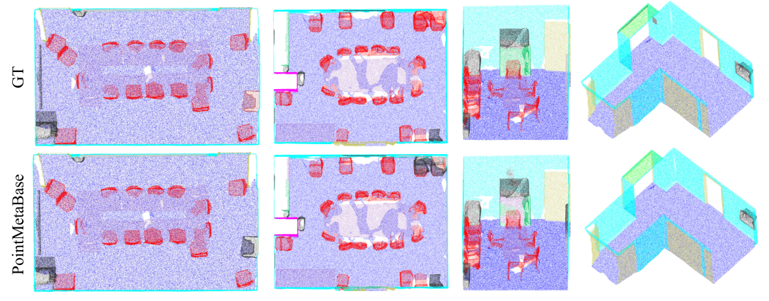
S3DIS s3dis is a challenging benchmark composed of 6 large-scale indoor areas, 271 rooms, and 13 semantic categories in total. The standard 6-fold cross-validation results and the Area-5 results on S3DIS are reported in Tab. 4. Since we adopt the same scaling strategies, PointMetaBase-L and PointMetaBase-XL have the same configuration on width and depth as PointNeXt-L and PointNeXt-XL. With only 13% FLOPs, our PointMetaBase-L outperforms PointNext-L by 1.7% and 0.8% in terms of mean IoU (mIoU) and overall accuracy (OA), respectively, and is much faster in terms of throughput. Compared with PointNext-XL, our PointMetaBase-XL uses only 11% of the FLOPs, but surpasses with 1.4% mIoU and 0.7% OA. The inference speed is faster. The excellent efficiency and performance of PointMetaBase can be attributed to the the removal of the computation redundancy in the two update functions and the improved position awareness introduced by explicit position embedding. ScanNet scannet contains 3D indoor scenes of various rooms with 20 semantic categories. The dataset is divided into 3 part: training, validation, and test splits, with 1201, 312 and 100 scans, respectively. Following PointNeXt pointnext, we do not use any voting strategies. As shown in Tab. 4, our PointMetaBase-L surpasses PointNeXt-L 1.6% mIoU with only 14% FLOPs and 1.7 faster inference speed. PointMetaBase-XL surpasses PointNeXt-XL 0.3% mIoU with only 11.3% FLOPs and 2.4 faster inference speed. Our largest variant, PointMetaBase-XXL, achieves better performance.
| Method |
|
|
|
|
| ||||||||||
|---|---|---|---|---|---|---|---|---|---|---|---|---|---|---|---|
| PointNet++ pointnet2 | 85.1 | 81.9 | 1.0 | 4.9 | - | ||||||||||
| KPConv kpconv | 86.4 | 85.1 | - | - | - | ||||||||||
| ASSANet assanet | 86.1 | - | - | - | - | ||||||||||
| Point Transformer pointtransformer | 86.6 | 83.7 | 7.8 | - | - | ||||||||||
| PointMLP pointmlp | 86.1 | 84.6 | - | - | - | ||||||||||
| StratifiedFormer stratified | 86.6 | 85.1 | - | - | - | ||||||||||
| PointNeXt-S pointnext | 86.7±0.0 | 84.4±0.2 | 1.0 | 4.5 | 873 | ||||||||||
| PointNeXt-S (C=64) pointnext | 86.9±0.1 | 84.8±0.5 | 3.7 | 17.8 | 391 | ||||||||||
| PointNeXt-S (C=160) pointnext | 87.0±0.1 | 85.2±0.1 | 22.5 | 110.2 | 118 | ||||||||||
| PointMetaBase-S (ours) | 86.7±0.0 | 84.3±0.1 | 1.0 | 1.39 | 1194 | ||||||||||
| PointMetaBase-S (C=64) (ours) | 86.9±0.1 | 84.9±0.2 | 3.8 | 3.85 | 706 | ||||||||||
| PointMetaBase-S (C=160) (ours) | 87.1±0.0 | 85.1±0.3 | 22.7 | 18.45 | 271 |
| Variants |
|
|
| ||||||
|---|---|---|---|---|---|---|---|---|---|
| PointNet++ pointnet2 | 77.9 | 1.7 | 2655 | ||||||
| PointCNN pointcnn | 78.5 | - | - | ||||||
| DGCNN dgcnn | 78.1 | 4.8 | 735 | ||||||
| DRNet pointnet | 80.3 | - | - | ||||||
| PointMLP pointmlp | 85.4±1.3 | 31.3 | 405 | ||||||
| PointNeXt-S pointnext | 87.7±0.4 | 1.7 | 2230 | ||||||
| PointMetaBase-S | 87.9±0.2 | 0.6 | 2674 |
5.2 3D Object Classification
ScanObjectNN scanobjectnn contains about 15000 real scanning objects, which are grouped into 15 classes and have 2902 unique instances. Following pointmlp; pointnext, we experiment on the hardest perturbed variant (PB_T50_RS). To make a fair comparison with PointNeXt pointnext, we did not use upscaled variants of PointMetaBase on this benchmark. As reported in Tab. 6, our model surpasses PointNeXt-S, while using much fewer model FLOPs and running much faster.
5.3 3D Part Segmentation
ShapeNetPart shapenetpart is a dataset for part segmentation of objects. It consists of 16880 models with 16 different shape categories. Each category has 2-6 parts and the number of total part labels is up to 50. Following the state-of-the-art method PointNeXt pointnext, we used voting by averaging the results of 10 randomly scaled input point clouds, with scaling factors equal to [0.8,1.2]. As shown in Tab. 5, compaerd with PointNeXt, our PointMetaBase family achieve comparable performance with large FLOPs reduction and faster inference speed. Specially, for C=32/C=64/C=160, the FLOPs of our PointMetaBase are only 30%21/%/17% that of PointNeXt, and the inference speed of PointMetaBase is 1.4/1.8/2.3 times faster than that of PointNeXt.
6 Conclusion
In this paper, we reformulate existing models for point cloud analysis into a general framework, PointMeta. Within this framework, we provide an in-depth analysis on the building blocks of existing models and summarize a few best practices for the building block design. Furthermore, we follow these best practices and propose a simple building block, PointMetaBase, which enjoys excellent performance and efficiency. The proposed framework and the simple block can encourage further rethinking and understanding on the building block design and shed new light on future architecture exploration.
References
- (1) Iro Armeni, Sasha Sax, Amir R. Zamir, and Silvio Savarese. Joint 2d-3d-semantic data for indoor scene understanding. CoRR, abs/1702.01105, 2017.
- (2) Peter W. Battaglia, Jessica B. Hamrick, Victor Bapst, Alvaro Sanchez-Gonzalez, Vinícius Flores Zambaldi, Mateusz Malinowski, Andrea Tacchetti, David Raposo, Adam Santoro, Ryan Faulkner, Çaglar Gülçehre, H. Francis Song, Andrew J. Ballard, Justin Gilmer, George E. Dahl, Ashish Vaswani, Kelsey R. Allen, Charles Nash, Victoria Langston, Chris Dyer, Nicolas Heess, Daan Wierstra, Pushmeet Kohli, Matthew M. Botvinick, Oriol Vinyals, Yujia Li, and Razvan Pascanu. Relational inductive biases, deep learning, and graph networks. CoRR, abs/1806.01261, 2018.
- (3) Xiangxiang Chu, Zhi Tian, Bo Zhang, Xinlong Wang, Xiaolin Wei, Huaxia Xia, and Chunhua Shen. Conditional positional encodings for vision transformers. arXiv preprint arXiv:2102.10882, 2021.
- (4) Angela Dai, Angel X. Chang, Manolis Savva, Maciej Halber, Thomas A. Funkhouser, and Matthias Nießner. Scannet: Richly-annotated 3d reconstructions of indoor scenes. In CVPR, pages 2432–2443. IEEE Computer Society, 2017.
- (5) Justin Gilmer, Samuel S. Schoenholz, Patrick F. Riley, Oriol Vinyals, and George E. Dahl. Neural message passing for quantum chemistry. In Doina Precup and Yee Whye Teh, editors, ICML, volume 70, pages 1263–1272, 2017.
- (6) Kaiming He, Xiangyu Zhang, Shaoqing Ren, and Jian Sun. Deep residual learning for image recognition. In CVPR, pages 770–778, 2016.
- (7) Qingyong Hu, Bo Yang, Linhai Xie, Stefano Rosa, Yulan Guo, Zhihua Wang, Niki Trigoni, and Andrew Markham. Randla-net: Efficient semantic segmentation of large-scale point clouds. In CVPR, pages 11105–11114, 2020.
- (8) Xin Lai, Jianhui Liu, Li Jiang, Liwei Wang, Hengshuang Zhao, Shu Liu, Xiaojuan Qi, and Jiaya Jia. Stratified transformer for 3d point cloud segmentation. In CVPR, pages 8490–8499. IEEE, 2022.
- (9) Guohao Li, Matthias Müller, Ali K. Thabet, and Bernard Ghanem. Deepgcns: Can gcns go as deep as cnns? In ICCV, pages 9266–9275, 2019.
- (10) Yangyan Li, Rui Bu, Mingchao Sun, Wei Wu, Xinhan Di, and Baoquan Chen. Pointcnn: Convolution on x-transformed points. In NeurIPS, pages 828–838, 2018.
- (11) Yongcheng Liu, Bin Fan, Shiming Xiang, and Chunhong Pan. Relation-shape convolutional neural network for point cloud analysis. In CVPR, pages 8895–8904, 2019.
- (12) Ze Liu, Han Hu, Yue Cao, Zheng Zhang, and Xin Tong. A closer look at local aggregation operators in point cloud analysis. In ECCV, pages 326–342, 2020.
- (13) Ze Liu, Yutong Lin, Yue Cao, Han Hu, Yixuan Wei, Zheng Zhang, Stephen Lin, and Baining Guo. Swin transformer: Hierarchical vision transformer using shifted windows. In ICCV, pages 9992–10002, 2021.
- (14) Xu Ma, Can Qin, Haoxuan You, Haoxi Ran, and Yun Fu. Rethinking network design and local geometry in point cloud: A simple residual MLP framework. In ICLR, 2022.
- (15) Charles Ruizhongtai Qi, Hao Su, Kaichun Mo, and Leonidas J. Guibas. Pointnet: Deep learning on point sets for 3d classification and segmentation. In CVPR, pages 77–85, 2017.
- (16) Charles Ruizhongtai Qi, Li Yi, Hao Su, and Leonidas J. Guibas. Pointnet++: Deep hierarchical feature learning on point sets in a metric space. In NeurIPS, pages 5099–5108, 2017.
- (17) Guocheng Qian, Hasan Hammoud, Guohao Li, Ali K. Thabet, and Bernard Ghanem. Assanet: An anisotropic separable set abstraction for efficient point cloud representation learning. In NeurIPS, pages 28119–28130, 2021.
- (18) Guocheng Qian, Yuchen Li, Houwen Peng, Jinjie Mai, Hasan Abed Al Kader Hammoud, Mohamed Elhoseiny, and Bernard Ghanem. Pointnext: Revisiting pointnet++ with improved training and scaling strategies. In NeurIPS, 2022.
- (19) Shi Qiu, Saeed Anwar, and Nick Barnes. Semantic segmentation for real point cloud scenes via bilateral augmentation and adaptive fusion. In CVPR, pages 1757–1767, 2021.
- (20) Karen Simonyan and Andrew Zisserman. Very deep convolutional networks for large-scale image recognition. In Yoshua Bengio and Yann LeCun, editors, ICLR, 2015.
- (21) Christian Szegedy, Vincent Vanhoucke, Sergey Ioffe, Jonathon Shlens, and Zbigniew Wojna. Rethinking the inception architecture for computer vision. In CVPR, pages 2818–2826, 2016.
- (22) Liyao Tang, Yibing Zhan, Zhe Chen, Baosheng Yu, and Dacheng Tao. Contrastive boundary learning for point cloud segmentation. In CVPR, pages 8479–8489, 2022.
- (23) Maxim Tatarchenko, Jaesik Park, Vladlen Koltun, and Qian-Yi Zhou. Tangent convolutions for dense prediction in 3d. In CVPR, pages 3887–3896, 2018.
- (24) Hugues Thomas, Charles R. Qi, Jean-Emmanuel Deschaud, Beatriz Marcotegui, François Goulette, and Leonidas J. Guibas. Kpconv: Flexible and deformable convolution for point clouds. In ICCV, pages 6410–6419, 2019.
- (25) Hugo Touvron, Matthieu Cord, Matthijs Douze, Francisco Massa, Alexandre Sablayrolles, and Hervé Jégou. Training data-efficient image transformers & distillation through attention. In ICML, pages 10347–10357, 2021.
- (26) Mikaela Angelina Uy, Quang-Hieu Pham, Binh-Son Hua, Duc Thanh Nguyen, and Sai-Kit Yeung. Revisiting point cloud classification: A new benchmark dataset and classification model on real-world data. In ICCV, pages 1588–1597, 2019.
- (27) Lei Wang, Yuchun Huang, Yaolin Hou, Shenman Zhang, and Jie Shan. Graph attention convolution for point cloud semantic segmentation. In CVPR, pages 10296–10305, 2019.
- (28) Shenlong Wang, Simon Suo, Wei-Chiu Ma, Andrei Pokrovsky, and Raquel Urtasun. Deep parametric continuous convolutional neural networks. In CVPR, pages 2589–2597, 2018.
- (29) Yue Wang, Yongbin Sun, Ziwei Liu, Sanjay E. Sarma, Michael M. Bronstein, and Justin M. Solomon. Dynamic graph CNN for learning on point clouds. ACM Trans. Graph., 38(5):146:1–146:12, 2019.
- (30) Kan Wu, Houwen Peng, Minghao Chen, Jianlong Fu, and Hongyang Chao. Rethinking and improving relative position encoding for vision transformer. In ICCV, pages 10013–10021, 2021.
- (31) Wenxuan Wu, Zhongang Qi, and Fuxin Li. Pointconv: Deep convolutional networks on 3d point clouds. In CVPR, pages 9621–9630, 2019.
- (32) Enze Xie, Wenhai Wang, Zhiding Yu, Anima Anandkumar, Jose M. Alvarez, and Ping Luo. Segformer: Simple and efficient design for semantic segmentation with transformers. In NeurIPS, pages 12077–12090, 2021.
- (33) Li Yi, Vladimir G. Kim, Duygu Ceylan, I-Chao Shen, Mengyan Yan, Hao Su, Cewu Lu, Qixing Huang, Alla Sheffer, and Leonidas J. Guibas. A scalable active framework for region annotation in 3d shape collections. ACM Trans. Graph., 35(6):210:1–210:12, 2016.
- (34) Hengshuang Zhao, Li Jiang, Chi-Wing Fu, and Jiaya Jia. Pointweb: Enhancing local neighborhood features for point cloud processing. In CVPR, pages 5565–5573, 2019.
- (35) Hengshuang Zhao, Li Jiang, Jiaya Jia, Philip H. S. Torr, and Vladlen Koltun. Point transformer. In ICCV, pages 16239–16248, 2021.
Supplementary Material
7 Limitation and Future Work
We further discuss the limitations of our work, which will be the focus in future. Firstly, although we find that explicit position embedding will promote performance significantly compared with other manners of position embedding, the rationale still remains unexplored. One possible direction is to look for theoretical explanations from gradient flows. Secondly, for the neighbor aggregation functions, we categorize them into learnable and non-learnable aggregation and find that the max pooling is a strong parameter-free method that is comparable to the learnable aggregation. Therefore, the next step is to do a finer taxonomy and richer ablation studies to find the applicable aggregation functions in different scenarios.
8 More Instantiation Examples
DGCNNdgcnn. The neighbor update is described as:
Different from PointNet++ pointnet2 that groups the neighbors in coordinate space, the neighbors grouping in DGCNN is conducted in the feature spaces. Similar to PointNet++, DGCNN uses max pooling as the neighbor aggregation function. The point update is absent in the DGCNN block. Additionally, there exists no position embedding function neither explicitly nor implicitly. In another word, there is no relative position information encoded in the output features.
PointCNNpointcnn. The neighbor update is described as:
The neighbor aggregation is defined as:
where denotes matrix multiplication and denotes the trainable convolution kernels of the convolution layer Conv. Two position embedding functions exist in this block. The first one is used in the neighbor update, while the second one is implicitly implemented by used in the neighbor aggregation function. Implementing position embedding by convolution layers is a common practice in the ViT family cpvt; segformer.
RandLA-Net randla. The neighbor update is described as follows:
The position embedding is described as:
The neighbor aggregation is implemented using attentive pooling that is similar to Point Transformer pointtransformer. The neighbor aggregation is as follows:
where denotes the attention weights for the neighbor , denotes the Hadamard product. Finally, the point feature is updated with an MLP layer and a shortcut, then we have
PointConv pointconv. The neighbor update and point update of PointConv is same with PointNet++ pointnet2. The original neighbor aggregation function of PointConv is defined as follow:
where is the weight matrices that map features from dimension to , denotes matrix multiplication, L denotes the number of the kernel points, denotes the coordinates of the kernel points, and denotes the associated weights matrices. However, different with the convolution for 2D images, the weight matrices in each local neighborhood for 3D is unique, which results in a huge memory cost. To address this challenge, the authors propose an efficient version, which decouples the weight matrix for each local neighborhood into two parts: a dynamic weight matrix and a static weight matrix . In this way, the memory consumption of the generated weights reduces to of the original version. The efficient version of neighbor aggregation is described as follows:
| (5) |
| (6) |
In Eq. 5, the neighbor features is transfomed into . Then, in Eq. 6, is turned into a vector by and then multiply with matrix .
where denotes matrix multiplication, denotes the number of the kernel points, denotes the coordinates of the kernel points, and denotes the associated weights matrices. Similar with the original version of PointConv pointconv, the dynamic weights matrices across all local neighborhoods will incur huge memory comsumption. Thus in the code implementation KPConv adopt similar strategy that first transforms the neighbor features with dynamic weights and then update point feature with static weights.
PointNeXtpointnext. PointNeXt conducts almost the same neighbor update with PointNet++ pointnet2 except for the configuration of the MLP. PointNet++ applies a 3-layer MLP while PointNeXt only applies 1 layer on the neighbor feature to reduce computation. Besides, PointNeXt also adopts a simple max pooling operation. As for the point update, PointNeXt uses a 2-layer MLP with an inverted bottleneck together with a shortcut layer from the input point feature , then we have:
9 Macro-Architecture
Applying explicit position embedding and the MLP-before-Group order, we tweak the set abstraction module pointnet2; pointnext as the reduction block, termed PointMetaSA. The decoder is composed of a series of feature propagation blocks pointnet2; pointnext. As shown in Fig. 3, a 1-layer MLP is used as stem in the first stage. In the later stages, PointMetaSA is placed first and the following are several PointMetaBase blocks. We adopt the same scaling strategies with PointNeXt pointnext to construct our PointMetaBase family. The configuration of our PointMetaBase family is summarized as follows:
- •
- •
- •
- •
denotes the channel size of the stem MLP and denotes the number of the PointMetaBase block in each stage. Note that when , only one PointMetaSA block but no PointMetaBase blocks are used at each stage. Due to the excellent efficiency of PointMetaBase, we do not need to construct the network at the level ”B” as done in PointNeXt pointnext. In contrast, we choose to scale the model to a larger level ”XXL”.