1Introduction

Improved Factorization for Threshold
Resummation in Heavy Quark to Heavy Quark Decays

U.G. Aglietti^(a) and G. Ferrera^(b)

^(a) Dipartimento di Fisica, Università di Roma “La Sapienza”,
I-00185 Rome, Italy

^(b) Dipartimento di Fisica, Università di Milano and
INFN Sezione di Milano, I-20133 Milan, Italy

We consider the resummation of soft-gluon effects in heavy quark to heavy quark decays, namely the processes $Q_{1}\to Q_{2}\,+\,\mathrm{(non\,QCD\,partons)}$ , where $Q_{1}$ and $Q_{2}$ are two different heavy quarks. We construct a new factorization scheme for threshold resummed spectra, which allows us to consistently evaluate the distribution of the final hadron invariant mass $m_{X}$ in all the kinematic regions, i.e. when $m_{X}$ is smaller, of the same order, or larger than the mass of the final quark $Q_{2}$ . A dependence of the Improved Coefficient Function on the threshold variable is introduced, which can however be relegated to a small interval of this variable by means of the so-called Partition of Unity. We explicitly apply our improved scheme to the $b\to X_{s}\,+\gamma$ decay at next-to-leading logarithmic accuracy.

1 Introduction

Analytic studies of Quantum-Chromo-Dynamics $(QCD)$ in the physical case, i.e. in four space-time dimensions, are substantially restricted to perturbation theory. The systematic application of perturbation theory to $QCD$ gives rise to the well-known perturbative Quantum-Chromo-Dynamics ( $pQCD$ ), a mature branch of theoretical physics, deeply involved in the phenomenology of the Standard Model. While exact analytic solutions of $QCD$ correlation functions could be intrinsically beyond human ability [1], perturbative calculations of cross sections and decay rates often reveal a rich structure and describe a variety of physical effects.

There are basically two different approaches in $pQCD$ . The first one involves an exact evaluation of the $QCD$ matrix elements of the process under investigation, up to a given order $n$ in the coupling $\alpha_{S}$ ( $n$ is taken, of course, as large as possible):

\sigma\,\simeq\,\sum_{k=0}^{n}\alpha_{S}^{k}\,\sigma^{(k)},

(1)

where $\sigma^{(k)}$ in the contribution to the physical cross section $\sigma=\sigma(\alpha_{S})$ of order $k$ . That way, all physical effects which show up in the matrix elements up to the truncation order $n$ are trivially taken into account. In this approach, one has to assume that the higher order $(k>n)$ contributions to the cross section can be safely neglected. In practice, one has to assume that all the terms in $\sigma^{(k)}$ are of order unity.

In the second approach, one concentrates instead, from the very beginning, on a specific physical effect. Usually, such effect manifests itself in peculiar perturbative terms, which depend on a kinematic parameter, and which become large in some region of the space of this parameter. Actually, at a generic order $k$ , such enhanced terms $s^{(k)}$ , contained in $\sigma^{(k)}$ , can become so large as to cancel the smallness of $\alpha_{S}^{k}$ , the $k$ -th power of the $QCD$ coupling. We face the situation

\alpha_{S}\,\ll\,1,\qquad\left|s^{(k)}\right|\,\gg\,1,

(2)

with:

\left|\alpha_{S}^{k}\,s^{(k)}\right|\,\raisebox{-3.0pt}{$\>\stackrel{{\scriptstyle>}}{{\scriptstyle\sim}}\>$}\,1,\quad\mathrm{for}\,\,k\,=\,1,\,2,\,3,\,\cdots.

(3)

For concreteness sake, we have assumed that the smallest order at which the physical effect under consideration manifests itself is one, i.e.

k\,\geq\,k_{\min}\,=\,1,

(4)

but higher values of $k_{\min}=2,3,\cdots$ , are possible; Usually, $k_{\min}$ is a small integer. In this physical situation, it is necessary to resum the enhanced terms $s^{(k)}$ to all orders of perturbation theory, i.e. for all $k$ . Schematically, we can write:

\sigma\,\simeq\,\sigma^{(0)}\,+\,\sum_{k=1}^{\infty}\alpha_{S}^{k}\,s^{(k)}.

(5)

Therefore, in the second approach, we realize an approximate resummation of the perturbative series of the given cross section to all orders. Note that, at each perturbative order $k$ , we do not compute the exact cross section contribution $\sigma^{(k)}$ , but only the leading term $s^{(k)}$ contained in it,

s^{(k)}\,\simeq\,\sigma^{(k)},

(6)

as far as the physical effect under consideration is taken into account.

From the above considerations, it should be clear that fixed-order calculations and resummed ones rely on quite different philosophies. In order to obtain an optimal perturbative description of the process, one should combine in some way the two approaches. That involves the so-called matching operation — or simply matching — in which one requires consistency between the two approaches. Roughly speaking, one would like to have an improved perturbative formula for the cross section which, at low orders, contains the exact matrix elements while, at higher orders, contains the approximate matrix elements of the resummation.

In this work we consider the general process

Q_{1}\,\to\,Q_{2}\,+\,\mathrm{(non\,QCD\,partons)},

(7)

where $Q_{1}$ and $Q_{2}$ are two different heavy quarks of mass $m_{1}$ and $m_{2}$ respectively and the non- $QCD$ , i.e. non colored, partons, can be a photon, a lepton pair, an intermediate vector boson, etc. For the decay to occur, one has to assume:

m_{2}\,<\,m_{1}.

(8)

Let us describe in qualitative terms the physics of the simplest process above as far as soft-gluon dynamics is concerned, namely the rare decay

B\,\to\,X_{s}\,+\,\gamma,

(9)

where $X_{s}$ is the final hadronic state containing the strange quark $s$ , coming from the fragmentation of the beauty quark $b$ inside the $B$ meson. In order to construct a general theory, let us assume that the strange quark mass $m_{s}$ is a parameter that we can change at will. Let us consider first the massless limit of the final quark,

m_{s}\,=\,0.

(10)

We assume to be in the so-called threshold (or large- $x$ ) region,

m_{X_{s}}^{2}\,\ll\,m_{b}^{2},

(11)

in which the invariant mass of the final hadronic (partonic in $pQCD$ ) state $X_{s}$ is restricted to be much smaller than the hard scale of the process, provided by the initial beauty quark mass, $Q=m_{b}$ . In terms of the normalized invariant mass squared

y\,\equiv\,\frac{m_{X_{s}}^{2}}{m_{b}^{2}}\qquad(m_{s}=0),

(12)

the threshold region is simply written:

y\,\ll\,1\qquad(y\in[0,1]).

(13)

Roughly speaking, in the threshold region, not much radiation can be emitted, so the related rate is expected to be suppressed. Note that we only fix the invariant mass $m_{X_{s}}$ of the final hadronic state, and not other quantities, such as for example the strange quark energy or its transverse momentum with respect to the photon 3-momentum. The final hadronic state $X_{s}$ is treated as a single pseudo-particle, with a continuous invariant mass distribution (rather than a fixed mass, like an ordinary particle). We may say that, by means of the condition (13), we observe $QCD$ radiation indirectly, in a semi-inclusive way.

The final strange quark, assumed to be emitted with a large energy compared to the $QCD$ scale $\Lambda_{QCD}\approx 300\,\mathrm{MeV}$ for $pQCD$ to be relevant,

E_{s}\,\approx\,\frac{m_{b}}{2}\,\gg\,\Lambda_{QCD},

(14)

evolves, because of collinear emissions, into a hadronic jet.

Let us now consider the rare decay (9) in the general massive case $m_{s}\neq 0$ . The situation becomes substantially more complicated because of the presence of a new mass scale. The definition of the threshold region (11) can be generalized by means of the condition

m_{X_{s}}^{2}\,-\,m_{s}^{2}\,\ll\,m_{b}^{2}\qquad(m_{s}\neq 0).

(15)

The invariant mass $m_{X_{s}}$ of the final hadronic state $X_{s}$ is restricted to not become much larger than $m_{s}$ , compared to the hard scale $m_{b}$ . As in the massless case, that is again a constraint on $QCD$ radiation: the latter cannot increase too much $m_{X_{s}}$ with respect to $m_{s}$ . Note that the condition above trivially reduces to (11) in the massless case, so it is a sensible generalization. Let us also remark that the condition (15) does not imply neither $m_{X_{s}}^{2}\ll m_{b}^{2}$ nor $m_{s}^{2}\ll m_{b}^{2}$ .

The unitary adimensional variable $y$ defined in eq.(12) is naturally generalized, in the massive case, as

y\,\equiv\,\frac{m_{X_{s}}^{2}\,-\,m_{s}^{2}}{m_{b}^{2}\,-\,m_{s}^{2}}\qquad\qquad(m_{s}\neq 0),

(16)

in terms of which the threshold region is written

y\,\ll\,1,

(17)

just like in the massless case. We have divided the squared mass increase, $m_{X_{s}}^{2}\,-\,m_{s}^{2}$ , by $m_{b}^{2}\,-\,m_{s}^{2}$ , instead of simply $m_{b}^{2}$ , in order to have a unitary variable $(y\in[0,1])$ , again as in the massless case.

If the final strange quark is relativistic (in the beauty rest frame), the non-vanishing of $m_{s}$ produces the well-known dead-cone ( $dc$ ) effect, i.e. the fact that gluon radiation is mostly emitted outside a cone centered around the strange quark motion direction, namely

\theta\,\raisebox{-3.0pt}{$\>\stackrel{{\scriptstyle>}}{{\scriptstyle\sim}}\>$}\,\theta_{\mathrm{dc}}\,=\,\frac{m_{s}}{E_{s}}\,=\,\frac{1}{\gamma_{s}}\,\ll\,1.

(18)

$\gamma_{s}$ is the Lorentz factor of the strange quark,

\gamma_{s}\,\equiv\,\frac{1}{\sqrt{1\,-\,\left|\vec{v}_{s}\right|^{\,2}/c^{2}}}\,\gg\,1,

(19)

with $\vec{v}_{s}\equiv d\vec{r}_{s}/dt$ the ordinary strange quark 3-velocity. The dead-cone effect is well known from classical electrodynamics [2]; In general, a non-vanishing final quark mass softens the collinear singularity according to a general mechanism [3]. Since the source of kinetic energy of the strange quark is the beauty mass, the strange quark can be relativistic only if it is much lighter than the beauty, i.e. if

m_{s}\,\ll\,m_{b}.

(20)

Since the usual kinematic condition of $y$ larger than a given positive value $y_{\mathrm{cut}}$ , namely

y\,>\,y_{\mathrm{cut}}\,>\,0,

(21)

also gives a constraint on gluon emission angles (the related observable is an infrared safe quantity), one has to find which one of the two limitations (18) and (21) is stronger and then effective.

In general, we can identify three different subregions in the threshold region (15).

1.

The effectively-massless region, in which the strange mass is much smaller than the final jet mass,

$m_{s}^{2}\,\ll\,m_{X_{s}}^{2}\,\ll\,m_{b}^{2}.$ (22)

In this case, the strange mass only gives power corrections to the massless distribution previously considered $(m_{s}=0)$ , of the form

$\left(\frac{m_{s}^{2}}{m_{X_{s}}^{2}}\right)^{n},\qquad n=1,2,3,\cdots,$ (23)

possibly multiplied by logarithms of the same quantity. As already remarked, since the invariant mass distribution is an infrared (i.e. soft and collinear) safe quantity, no strange quark mass singularities can arise (i.e. terms of the form $\log m_{s}^{2}/m_{X_{s}}^{2}$ without a power-suppressed coefficient). In this case, the strange mass is so small that the dead-cone effect (18) gives a small correction to the massless distribution. Note that relation (22) is basically equivalent to the relation

$m_{s}^{2}\,\ll\,m_{X_{s}}^{2}\,-\,m_{s}^{2}\,\ll\,m_{b}^{2}\,-\,m_{s}^{2}\approx m_{b}^{2}.$ (24)

If we define the mass-correction parameter

$\rho\,\equiv\,\frac{m_{s}^{2}}{m_{b}^{2}\,-\,m_{s}^{2}}\qquad(0<\rho<\infty),$ (25)

the region (22) is simply written

$\rho\,\ll\,y\,\ll\,1.$ (26)
2.

The quasi-collinear slice, in which the increase of the jet invariant mass produced by soft-gluon radiation is comparable to the strange quark mass,

$m_{X_{s}}^{2}\,-\,m_{s}^{2}\,\approx\,m_{s}^{2}\,\ll\,m_{b}^{2},$ (27)

or, equivalently,

$\rho\,\approx\,y\,\ll\,1.$ (28)

Formally, one can consider the (correlated) limit:

$y\,\to\,0^{+},\qquad\rho\,\to\,0^{+},\qquad\frac{\rho}{y}\,\to\,\mathrm{const},$ (29)

where $\mathrm{const}\neq 0,\infty$ . This is a double-logarithmic region, as the previous one or the massless case.
3.

The soft region, in which the increase in the final jet mass due to gluon radiation is much smaller than the strange mass,

$m_{X_{s}}^{2}\,-\,m_{s}^{2}\,\ll\,m_{s}^{2}.$ (30)

In terms of the adimensional variables we have introduced, the above condition is written:

$y\,\ll\,\rho.$ (31)

Since we always assume $y\ll 1$ , the above relation basically implies one of the two following possibilities:

$\rho\,\approx\,1\quad\mathrm{or}\quad\rho\,\gg\,1.$ (32)

Since the final strange quark is not relativistic in any of the two above cases, there is not any collinear enhancement in this region. At any order of perturbation theory, one finds at most, in the invariant mass distribution, one large infrared logarithm of soft origin for each power of $\alpha_{S}$ . In other words, this region is a single-logarithmic, rather than a double-logarithmic, one¹¹ 1 The situation is analogous to Deep Inelastic Scattering $(DIS)$ (even though the latter is not a collinear safe process), where soft singularities, unlike collinear ones, cancel in the inclusive cross section. Therefore the perturbative expansion of the latter contains at most one large infrared logarithm of collinear origin for each power of $\alpha_{S}$ [4]. . If $\rho\gg 1$ , the final quark is very slow (in the initial quark rest frame) and soft-gluon radiation is suppressed by color coherence. Soft gluons indeed ”see” a static color charge which, at the fragmentation time, begins to move with a very small velocity, without any color-spin flip. In the limit of vanishing final velocity, soft gluons just see a static color charge at any time.

The paper is organized as follows. In sec. 2 we discuss the main phenomenological applications of our work. Nature provides to us heavy quark decays with quite different mass ratios, so we conclude that our work is not academic.

In sec. 3 we consider threshold resummation in the massless limit of the final quark, $m_{2}=0$ . As already anticipated, this case is considerably simpler than the massive case $m_{2}\neq 0$ , which is our primary concern. This is a preliminary section written in order to present the main ideas in a simple case and to fix the notation. This section also has a pedagogical character and can be omitted by an expert on threshold resummation.

In sec. 4 we describe the exact calculation to first-order in $\alpha_{S}$ , of the photon energy spectrum in the rare $B\to X_{s}\gamma$ decay, which is assumed as a model process. As already remarked, the above process is selected because of its simplicity, but we believe that the main consequences which we derive can be generalized to more complicated processes in the class (7), and perhaps even more.

In sec. 5 we consider threshold resummation, in the usual rare decay, in the soft limit. As already remarked, that means, that the (massive) final quark is produced, in the fragmentation of the initial heavy quark (at rest), with a non-relativistic velocity. We may say that the latter is a complementary situation with respect to the massless limit of the final quark.

In sec. 6 we construct a general factorization scheme in the massive case. We introduce, as usual, a universal, i.e. process independent, long-distance dominated $QCD$ Form factor, resumming the infrared logarithms to all orders in $\alpha_{S}$ , together with a Coefficient and a Remainder functions. Unlike the form factor, the latter are process-dependent, short-distance quantities, having an ordinary (i.e. truncated) perturbative expansion.

Sec. 7 is the central one, the core of the paper. In this section we consider the problems of the general massive factorization scheme, constructed in the previous section, concerning the massless limit of the final quark, $m_{2}\to 0$ , which turns out not to be correctly reproduced. An improved factorization scheme is then constructed which reproduces, in the massless limit, the factorization of the massless process discussed in sec. 3. The main point is that, as we are going to show, it is necessary to introduce a dependence, inside the Coefficient function, on the final hadron invariant mass, i.e. on the variable $y$ .

Finally, sec. 8 contains the conclusions of our analysis, together with a discussion about future developments. In general, a lot of work along the lines of this paper remains to be made. The main developments which we can foresee, involve the application of the improved factorization scheme to other processes than $B\to X_{s}\gamma$ decays, as well as the generalization of the scheme to higher orders.

2 Phenomenological Relevance

As far as soft-gluon effects are concerned, the hard scale $Q$ of the process (7), in the rest frame of the initial heavy quark $Q_{1}$ ( $\vec{p}_{1}=0$ ), is given by [5, 6, 7, 8, 9, 10]:

Q\,=\,E_{X}\,+\,\left|\vec{p}_{X}\right|,

(33)

where, as already defined, $X$ denotes the final hadronic state into which the quark $Q_{2}$ evolves (basically, a hadronic jet). If we denote by $q^{\mu}$ the total 4-momentum of the non QCD partons, the hard scale can be written:

Q\,=\,m_{1}\,-\,\sqrt{q^{2}\,+\,\left|\vec{q}\,\right|^{2}}\,+\,\left|\vec{q}\,\right|\,=\,m_{1}\,-\,q_{0}\,+\,\sqrt{q_{0}^{2}\,-\,q^{2}},

(34)

where

q^{2}\,\equiv\,q^{\mu}q_{\mu}\,=\,q_{0}^{2}\,-\,\left|\vec{q}\,\right|^{2}

(35)

is the invariant mass squared of the non QCD partons. Note that, for large values of $q^{2}$ , the non colored particles can take away a substantial fraction of the available energy from the $QCD$ subprocess, reducing to a large extent the hard scale $Q$ from the ”natural” or upper value $m_{1}$ :

q^{2}\,\raisebox{-3.0pt}{$\>\stackrel{{\scriptstyle<}}{{\scriptstyle\sim}}\>$}\,m_{1}^{2}\quad\Rightarrow\quad Q^{2}\,\ll\,m_{1}^{2}.

(36)

In the real world, one may cite the following cases of heavy-to-heavy decays (7):

1.

The rare (one-loop mediated) beauty quark decays

$b\,\to\,X_{s}\,+\,\gamma,$ (37)

which we have already considered in the Introduction. In the real world, if we take a constituent (i.e. large) strange quark mass $m_{s}\approx 500\,\mathrm{MeV}$ (let’s say, one half of the $\Phi$ mass), the quark mass ratio

$\frac{m_{s}}{m_{b}}\,\approx\,\frac{1}{10}.$ (38)

In this process, since the photon is real, the 4-momentum $q^{\mu}$ of the probe is light-like, $q^{2}=0$ , so the hard scale $Q$ , according to eq.(34), exactly coincides with the beauty mass:

$Q\,=\,m_{b};$ (39)
2.

The $CKM$ -favored semileptonic $b$ decays

$b\,\to\,X_{c}\,+\,l\,+\,\nu,$ (40)

where $X_{c}$ is the final hadronic state containing the charm quark, coming from beauty fragmentation, with the (rather large) quark mass ratio

$\frac{m_{c}}{m_{b}}\,\approx\,\frac{1}{3}.$ (41)

As already noted, the lepton pair can take away a considerable energy from the $QCD$ subprocess. Unlike previous case 1, according to eq.(34), the true hard scale

$Q\,=\,E_{X_{c}}\,+\,\left|\vec{p}_{X_{c}}\right|,$ (42)

is substantially smaller than the beauty mass $m_{b}$ for a large dilepton invariant mass, $q^{2}\raisebox{-3.0pt}{$\>\stackrel{{\scriptstyle<}}{{\scriptstyle\sim}}\>$}m_{b}^{2}$ ;
3.

As a final example of (7), let us mention the $CKM$ -favored top quark decays

$t\,\to\,b\,+\,W,$ (43)

where the heavy quark mass ratio is very small:

$\frac{m_{b}}{m_{t}}\,\approx\,\frac{1}{35}.$ (44)

We may conclude that phenomenology offers a rather wide class of processes (7), with quite spread values of the quark mass ratio.

3 Massless Case

For simplicity’s sake, let us begin our analysis considering the rare decay (37) in the massless limit of the final strange quark,

m_{s}\,=\,0.

(45)

In this heavy-to-light decay, both fixed-order and resummed calculations greatly simplify. Again for simplicity’s sake, let us approximate the effective weak nonleptonic Hamiltonian governing the decay (37) by keeping only the local operator

	$\displaystyle O_{7}(x)$	$\displaystyle\equiv$	$\displaystyle\frac{e}{16\,\pi^{2}}\,\bar{s}_{i}(x)\,\sigma^{\mu\nu}\left(m_{b}\,R\,+\,m_{s}\,L\right)b^{i}(x)\,F_{\mu\nu}(x)\,=\,$		(46)
		$\displaystyle=$	$\displaystyle\frac{e\,m_{b}}{16\,\pi^{2}}\,\bar{s}_{i}(x)\,\sigma^{\mu\nu}R\,b^{i}(x)\,F_{\mu\nu}(x)\qquad\qquad\qquad\qquad\qquad\qquad\qquad(m_{s}=0),$		(46)

where $e$ is the proton charge and we have defined the standard Right $(R)$ and Left $(L)$ projectors:

R\,\equiv\,\frac{1\,+\,\gamma_{5}}{2};\qquad L\,\equiv\,\frac{1\,-\,\gamma_{5}}{2}.

(47)

The generalization to all the operators in the effective Hamiltonian will be discussed in sec. 7.3.

3.1 Total decay rate

The tree-level width of the rare decay (37) reads:

\Gamma^{(0)}_{0}\,=\,\frac{G_{F}^{2}m_{b}^{5}}{32\,\pi^{3}}\,C_{7}^{2}\,\left|\lambda_{t}\right|^{2}\,\frac{\alpha_{em}}{\pi},

(48)

where $G_{F}$ is the Fermi constant, $m_{b}$ is the on-shell beauty mass, $\alpha_{em}\approx 1/137$ is the fine-structure constant and the constant $C_{7}$ is the Wilson (short-distance) Coefficient function of the operator $O_{7}$ , resumming large logarithms of $m_{w}/m_{b}$ to all orders, as well as collecting finite corrections. Finally $\lambda_{t}$ is a product of $CKM$ matrix elements:

\lambda_{t}\,\equiv\,V_{tb}V_{ts}^{*},

(49)

Through the paper, we use the following conventions: the lower index zero, on the l.h.s. of eq.(48) for example, refers to the massless limit. In general, we will denote quantities calculated in the $m_{s}=0$ limit with a zero subscript. The upper index, between round brackets, denotes instead the order in perturbation theory.

3.2 Photon spectrum or invariant hadron squared mass distribution

We consider the invariant hadron squared-mass spectrum, paying particular attention to the low-mass or threshold region

m_{X_{s}}^{2}\,\ll\,m_{b}^{2}.

(50)

As already noted, the hard scale $Q$ is given by the beauty mass $m_{b}$ , as:

Q\,=\,E_{X_{s}}\,+\,|\vec{p}_{X_{s}}|\,=\,m_{b}\,-\,E_{\gamma}\,+\,|\vec{p}_{\gamma}|\,=\,m_{b}\qquad(c=1).

(51)

Since, at lowest order in the $QCD$ coupling $\alpha_{S}$ , there is no gluon radiation, the final hadronic state only contains the strange quark,

\alpha_{S}\,=\,0:\quad X_{s}\,=\,s,

(52)

so that:

m_{X_{s}}^{2}\,=\,m_{s}^{2}\,=\,0.

(53)

By defining the unitary variable

y\,\equiv\,\frac{m_{X_{s}}^{2}\,-\,m_{s}^{2}}{m_{b}^{2}\,-\,m_{s}^{2}}\,=\,\frac{m_{X_{s}}^{2}}{m_{b}^{2}}\qquad(m_{s}=0),

(54)

it follows that the tree-level (i.e. lowest-order) spectrum is a spike at vanishing $y$ :

\frac{d\Gamma_{0}^{(0)}}{dy}\,=\,\Gamma^{(0)}_{0}\,\delta(y).

(55)

In general, the differential spectrum in $y$ has a perturbative expansion in powers of $\alpha_{S}$ of the form:

\frac{d\Gamma_{0}}{dy}\left(y;\alpha_{S}\right)\,=\,\Gamma_{0}^{(0)}\,\delta(y)\,+\,\sum_{n=1}^{\infty}C_{F}\left(\frac{\alpha_{S}}{\pi}\right)^{n}\frac{d\Gamma_{0}^{(n)}}{dy}(y)\qquad(0\leq y\leq 1),

(56)

where $C_{F}=(N^{2}-1)/(2N)=4/3$ for $N=3$ colors in $QCD$ . In the beauty rest frame ( $p_{b}^{\mu}=(m_{b};0,0,0)$ ), by elementary kinematics:

E_{\gamma}\,=\,\frac{m_{b}^{2}\,-\,m_{X_{s}}^{2}}{2m_{b}}\,=\,\frac{m_{b}}{2}\left(1\,-\,\frac{m_{X_{s}}^{2}}{m_{b}^{2}}\right).

(57)

By defining the unitary variable

x\,\equiv\,\frac{E_{\gamma}}{\,E_{\gamma}^{\max}}\,=\,1\,-\,\frac{m_{X_{s}}^{2}}{m_{b}^{2}}\qquad(0\leq x\leq 1),

(58)

we find the relation

x\,=\,1\,-\,y\qquad(m_{s}=0).

(59)

Therefore, to evaluate the hadron squared mass distribution is equivalent to compute the photon energy spectrum. In the high-mass region, the emitted photon is soft, while in the low-mass region (50), the photon is hard, i.e. its energy $E_{\gamma}$ is close to its upper endpoint $m_{b}/2$ , so that:

E_{\gamma}^{\min}\,=\,0;\qquad E_{\gamma}^{\max}\,=\,\frac{m_{b}}{2}\qquad(m_{s}=0).

(60)

For technical reasons (to avoid distributions), it is simpler to consider the normalized, partially-integrated spectrum, the so-called event fraction:

E_{0}(y;\alpha_{S})\,\equiv\,\frac{1}{\Gamma_{0}}\int\limits_{0}^{y}\frac{d\Gamma_{0}}{dy^{\prime}}(y^{\prime};\alpha_{S})\,dy^{\prime}\qquad(0\leq y\leq 1).

(61)

The differential spectrum is simply obtained by differentiation of the event fraction:

\frac{1}{\Gamma_{0}}\frac{d\Gamma_{0}}{dy}\,=\,\frac{dE_{0}}{dy}.

(62)

It follows directly from the definition of event fraction given in eq.(61) that:

\lim_{y\to 0^{+}}E_{0}(y;\alpha_{S})\,=\,0;\qquad\lim_{y\to 1^{-}}E_{0}(y;\alpha_{S})\,=\,1.

(63)

By integrating both sides of eq.(55) with respect to $y$ , it is immediately found that the tree-level event fraction is identically equal to one for any $y>0$ :

E_{0}^{(0)}(y)\,\equiv\,\frac{1}{\Gamma_{0}^{(0)}}\int\limits_{0}^{y}\frac{d\Gamma_{0}^{(0)}}{dy^{\prime}}\,dy^{\prime}\,=\,\theta(y)\,\equiv\,1\qquad(y>0);

(64)

where $\theta(y)\equiv 1$ for $y>0$ and zero otherwise is the standard Heaviside unit-step function.

The event fraction at first order in $\alpha_{S}$ only depends on diagrams involving single real gluon emission (bremmstrahlung), as:

E_{0}(y;a)\,=\,\frac{\Gamma_{0}^{(0)}\,+\,a\,\int\limits_{0}^{y}dy^{\prime}\,d\Gamma_{0}^{(1)}/dy^{\prime}\,+\,\mathcal{O}\left(a^{2}\right)}{\Gamma_{0}^{(0)}\,+\,a\,\int\limits_{0}^{1}dy\,d\Gamma_{0}^{(1)}/dy\,+\,\mathcal{O}\left(a^{2}\right)}\,=\,1\,-\,\frac{a}{\Gamma_{0}^{(0)}}\,\int\limits_{y}^{1}\frac{d\Gamma_{0}^{(1)}}{dy^{\prime}}\,dy^{\prime}\,+\,\mathcal{O}\left(a^{2}\right)\qquad(y>0);

(65)

where we have defined the effective, first-order coupling of the (heavy) quarks to gluons

a\,\equiv\,\frac{C_{F}\alpha_{S}}{\pi}.

(66)

We may say that the event fraction and the total rate give complementary information about the decay process. Note that the second equation in (63) is trivially satisfied by eq.(65). To verify the first equation is instead less trivial. To accomplish this task, one has to resum soft-gluon effects to all orders in $\alpha_{S}$ , as we are going to show.

An exact first-order calculation in $\alpha_{S}$ or, equivalently, in $a$ , of the event fraction gives [11, 12]:

	$\displaystyle E_{0}\left(y;a\right)\,=\,1$	$\displaystyle-$	$\displaystyle\frac{a}{2}\,\log^{2}(y)\,-\,\frac{7}{4}\,a\,\log(y)\,-\,a\,\frac{31}{12}\,+$		(67)
		$\displaystyle-$	$\displaystyle a\bigg[\,y\left(1\,-\,\frac{y}{4}\right)\log(y)\,+\,\frac{y}{12}\left(2\,y^{2}\,-\,3\,y\,-\,30\right)\bigg]\,+\,\mathcal{O}\left(a^{2}\right).$		(67)

The spectrum above contains three different kind of terms, as far as the Born-kinematics limit $y\to 0^{+}$ is concerned:

1.

Double and single logarithmic terms of $y$ , namely the terms

$-\,\frac{a}{2}\,\log^{2}(y),\qquad\,-\,\frac{7}{4}\,a\,\log(y),$ (68)

which formally diverge in the limit $y\to 0^{+}$ , and which are therefore very large in the lower end-point region $y\ll 1$ — namely the threshold region. These are clearly the dominant terms in the small- $y$ region;
2.

Constant terms with respect to $y$ , namely the term

$\,-\,a\,\frac{31}{12}.$ (69)

In units of the ubiquitous factor $a$ , the constant

$C^{(1)}_{0}\,=\,-\,\frac{31}{12}\,\cong\,-\,2.6$ (70)

is of order one, as expected. For $\alpha_{S}(m_{b})=0.21$ , the first-order correction turns out to be

$a\,C^{(1)}_{0}\,\simeq\,-\,0.23;$ (71)

Infinitesimal terms in $y$ , i.e. terms which vanish in the limit $y\to 0^{+}$ , namely

a\,H^{(1)}_{0}(y),

(72)

where:

H^{(1)}_{0}(y)\,\equiv\,-\,y\left(1\,-\,\frac{y}{4}\right)\log(y)\,-\,\frac{y}{12}\left(2\,y^{2}\,-\,3\,y\,-\,30\right).

(73)

These latter terms are the least important ones in the small- $y$ region, but give a substantial contribution in the bulk of the spectrum, i.e. for $y=\mathcal{O}(1)$ . These terms can be neglected, to a first approximation, in the small- $y$ region, but cannot be neglected anymore for generic $y$ values, where they are not smaller than the logarithmic or the constant terms.

As far as the small- $y$ behavior is concerned, in the general process (7), the event fraction is naturally written to first order in the form

E_{0}(y;a)\,=\,1\,-\,\frac{a}{2}\,A^{(1)}\log^{2}(y)\,+\,a\,S^{(1)}\log(y)\,+\,a\,C^{(1)}_{0}\,+\,a\,\mathrm{Rem}^{(1)}_{0}(y)\,+\,\mathcal{O}\left(a^{2}\right);

(74)

where we have introduced the coefficients:

A^{(1)}\,=\,1;\qquad S^{(1)}\,=\,-\,\frac{7}{4}.

(75)

The value of the constant $C^{(1)}_{0}$ has already been given in eq.(70) and the first-order contribution to the remainder function

\mathrm{Rem}^{(1)}_{0}(y)\,\equiv\,H^{(1)}_{0}(y)\,\to\,0\,\,\,\mathrm{for}\,\,y\,\to\,0^{+}.

(76)

The complete Remainder function at first order,

\mathrm{Rem}_{0}(y;a)\,=\,a\,\mathrm{Rem}^{(1)}_{0}(y),

(77)

is plotted in fig. 1. Note that, since $E_{0}(y=1,a)\equiv 1$ , it follows that:

\mathrm{Rem}^{(1)}_{0}(y=1)\,=\,-\,C^{(1)}_{0}\,=\,\frac{31}{12}.

(78)

Actually, the Remainder Function is a strictly-monotonically-increasing function of $y$ , and therefore positive in all its range, $0\leq y\leq 1$ .

Refer to caption — Figure 1: Plot of Massless Remainder Function $\mathrm{Rem}_{0}(y;a)$ in first approximation, eq.(77), as a function of $y$ in all its kinematic range, $0\leq y\leq 1$ . We have defined $a\equiv C_{F}\alpha_{S}(m_{b})/\pi\cong 0.089$ for $\alpha_{S}(m_{b})=0.21$ .

The constants $A^{(1)}$ and $S^{(1)}$ are process-independent, i.e. they are the same for all the heavy-to-light decays in the class (7). That is a consequence of the general properties of $QCD$ radiation in the infrared (i.e. soft and/or collinear) limit. On the contrary, the Coefficient $C^{(1)}_{0}$ and the Remainder function $\mathrm{Rem}^{(1)}_{0}(y)$ are short-distance dominated and are therefore process dependent.

In the simple case of the radiative decay (37) – a two-body decay at tree level – $C^{(1)}_{0}$ is truly a constant and $\mathrm{Rem}^{(1)}_{0}(y)$ only depends on $y$ . In more complicated heavy-to-light decays, such as for example the semileptonic $b\to ul\nu$ decays – 3-body decays at tree-level – $C^{(1)}$ still does not depend on $y$ , but it does depend on other kinematical variables. Similarly, the Remainder function $\mathrm{Rem}^{(1)}(y)$ also depends on additional kinematical variables.

3.3 Factorization

The basic idea of factorization is simply to separate from each other perturbative terms having different physical origin. In particular, we factorize the large infrared logarithms into a universal, i.e. process independent, form factor. To order $a$ (i.e. to order $\alpha_{S}$ ), one can write indeed:

E_{0}(y;a)\,=\,C_{0}(a)\,\Sigma_{0}(y;a)\,+\,\mathrm{Rem}_{0}(y;a)\,+\,\mathcal{O}\left(a^{2}\right);

(79)

where we have defined the long-distance dominated $QCD$ form factor

\Sigma_{0}(y;a)\,\equiv\,1\,-\,\frac{a}{2}\,A^{(1)}\log^{2}(y)\,+\,a\,S^{(1)}\log(y);

(80)

the short-distance Coefficient function:

C_{0}(a)\,\equiv\,1\,+\,a\,C^{(1)}_{0}

(81)

and the short-distance Remainder function

\mathrm{Rem}_{0}(y;a)\,\equiv\,a\,H^{(1)}_{0}(y).

(82)

Note that the perturbative expansion of the Remainder function begins at order $a$ , i.e. it vanishes in the free limit $a\to 0$ , while the Form factor and the Coefficient function equal unity in the same limit.

By expanding the product on the r.h.s. of eq.(79) in powers of $a$ , one finds:

E_{0}(y;a)\,=\,1\,+\,a\,\Sigma_{0}^{(1)}(y)\,+\,a\,C^{(1)}_{0}\,+\,a\,\mathrm{Rem}^{(1)}_{0}(y)\,+\,\mathcal{O}\left(a^{2}\right).

(83)

On the r.h.s. of the above equation, one finds exactly the same first-order terms which are on the r.h.s. of the fixed-order expansion, eq.(74). Therefore factorization, which we have explicitly constructed at first order in $a$ , involves a shift of terms of second (and in general also higher) order.

Let us note that we have constructed a minimal scheme for the $QCD$ form factor $\Sigma_{0}(y;a)$ , inside which only logarithmic terms of $y$ are included. In other words, constants and infinitesimal terms for $y\to 0^{+}$ are not included in our $\Sigma_{0}$ . Let us also remark that the factorization scheme given by eq.(79) can be consistently pushed to higher orders in $\alpha_{S}$ .

3.4 Threshold resummation in the heavy-to-light case

The $QCD$ form factor, resumming to all orders in $\alpha_{S}$ the infrared logarithmically-enhanced terms, has the standard expression in moment space or $N$ -space [13, 14, 15, 5]:

	$\displaystyle\sigma_{0,N}\left(\alpha_{S}\right)$	$\displaystyle=$	$\displaystyle\exp\int\limits_{0}^{1}\frac{dy}{y}\Big[(1-y)^{N-1}\,-\,1\Big]\Bigg\{\,\,\int\limits_{Q^{2}y^{2}}^{Q^{2}y}\frac{dk_{\perp}^{2}}{k_{\perp}^{2}}\,A\left[\alpha_{S}\left(k_{\perp}^{2}\right)\right]\,+$		(84)
			$\displaystyle\qquad\qquad\qquad\qquad\qquad\qquad\,+\,B\left[\alpha_{S}\left(Q^{2}y\right)\right]\,+\,D\left[\alpha_{S}\left(Q^{2}y^{2}\right)\right]\Bigg\}.$		(84)

The function $A(\alpha_{S})$ , having an ordinary perturbative expansion in powers of $\alpha_{S}$ ,

A(\alpha_{S})\,=\,\sum_{n=1}^{\infty}C_{F}\left(\frac{\alpha_{S}}{\pi}\right)^{n}\,A^{(n)},

(85)

describes soft-gluon emission at small angle with respect to the parent strange quark [16] (i.e. both soft and collinear enhanced). The first-order coefficient $A^{(1)}$ – the only one we are directly interested to – has been given in the first of eqs.(75), in units of $a\equiv C_{F}\alpha_{S}/\pi$ , according to our current conventions.

The function $B(\alpha_{S})$ , also having an ordinary perturbative expansion in powers of $\alpha_{S}$ ,

B(\alpha_{S})\,=\,\sum_{n=1}^{\infty}C_{F}\left(\frac{\alpha_{S}}{\pi}\right)^{n}\,B^{(n)}\,=\,a\,B^{(1)}\,+\,\mathcal{O}\left(a^{2}\right),

(86)

describes hard-gluon emission at small angle (collinear enhanced but not soft enhanced radiation). The first-order coefficient explicitly reads:

B^{(1)}\,=\,-\,\frac{3}{4}.

(87)

Finally, the function $D(\alpha_{S})$ , also having an ordinary perturbative expansion in powers of $\alpha_{S}$ ,

D(\alpha_{S})\,=\,\sum_{n=1}^{\infty}C_{F}\left(\frac{\alpha_{S}}{\pi}\right)^{n}\,D^{(n)}\,=\,a\,D^{(1)}\,+\,\mathcal{O}\left(a^{2}\right),

(88)

describes soft-gluon emission at large angle (soft enhanced but not collinear enhanced radiation). In heavy-to-light transitions, the first-order coefficient takes the value:

D^{(1)}\,=\,-\,1.

(89)

It is natural to resum infrared logarithms in $N$ -space, where, unlike physical space, factorization of kinematic constraints for multiple soft-gluon emission holds true [17]. In $N$ -space, the logarithm-enhanced terms have the form

\alpha_{S}^{k}\,\log^{l}(N),\qquad k\,=\,1,\,2,\,3,\,\cdots,\quad 1\,\leq\,l\,\leq\,2\,k.

(90)

As well known, in order to obtain the form factor in physical space ( $y$ -space), one has to make first analytic continuation of $\sigma_{N}$ in the $N$ variable, from integer to complex values:

N\in{\mathbb{N}}\quad\mapsto\quad\mathcal{N}\in{\mathbb{C}}.

(91)

The form factor in physical space is then obtained by means of an inverse Mellin transform:

\sigma_{0}(y;\alpha_{S})\,=\,\int\limits_{c-i\infty}^{c+i\infty}\frac{d\mathcal{N}}{2\pi i}\,(1-y)^{-\mathcal{N}}\sigma_{0,\mathcal{N}}(\alpha_{S}),

(92)

where the (real) constant $c$ is chosen in such a way that all the singularities of $\sigma_{\mathcal{N}}$ lie to the left of the integration contour (a vertical line in the complex $\mathcal{N}$ -plane).

The partially-integrated form factor $\Sigma_{0}(y)$ is finally obtained by integrating over $y$ :

\Sigma_{0}(y;\alpha_{S})\,=\,\int\limits_{0}^{y}\sigma_{0}(y^{\prime};\alpha_{S})\,dy^{\prime}.

(93)

3.4.1 Form-factor expansion

In order to determine the first-order Coefficient and Remainder functions, one has to subtract, from the event fraction, the expansion of the form factor up to first order in $\alpha_{S}$ .

The first step involves expanding the exponential on the r.h.s. of eq.(84) to first order,

\sigma_{0,N}\,=\,\exp(X)\,=\,1\,+\,X\,+\,\mathcal{O}\left(X^{2}\right),

(94)

followed by a truncation of the resummation functions $A(\alpha_{S}),B(\alpha_{S})$ and $D(\alpha_{S})$ to first order in $\alpha_{S}$ :

$\displaystyle\sigma_{0,N}(\alpha_{S})$	$\displaystyle=$	$\displaystyle 1\,+\,\int\limits_{0}^{1}\frac{dy}{y}\big[(1-y)^{N-1}\,-\,1\big]\Bigg\{\,\,\int\limits_{Q^{2}y^{2}}^{Q^{2}y}\frac{dk_{\perp}^{2}}{k_{\perp}^{2}}\,A\left[\alpha_{S}\left(k_{\perp}^{2}\right)\right]\,+$	(95)
		$\displaystyle\qquad\qquad\qquad\qquad\qquad\,+\,B\left[\alpha_{S}\left(Q^{2}y\right)\right]\,+\,D\left[\alpha_{S}\left(Q^{2}y^{2}\right)\right]\Bigg\}\,+\,\mathcal{O}\left(\alpha_{S}^{2}\right)\,=$
	$\displaystyle=$	$\displaystyle 1\,+\,a\,\int\limits_{0}^{1}dy\big[(1-y)^{N-1}\,-\,1\big]\Bigg\{\,\,\frac{A^{(1)}}{y}\int\limits_{Q^{2}y^{2}}^{Q^{2}y}\frac{dk_{\perp}^{2}}{k_{\perp}^{2}}\,+\,\frac{B^{(1)}\,+\,D^{(1)}}{y}\Bigg\}\,+\,\mathcal{O}\left(a^{2}\right);$

where:

\alpha_{S}\,\equiv\,\alpha_{S}\left(Q^{2}\right);\qquad a\,\equiv\,\frac{C_{F}\,\alpha_{S}\left(Q^{2}\right)}{\pi}.

(96)

Since $X=\mathcal{O}\left(\alpha_{S}\right)$ , the higher-order terms $X^{2},X^{3},\cdots$ in the expansion of $\exp(X)$ are of second or higher order in $\alpha_{S}$ . The evaluation of the inverse Mellin transform simply gives back, at first order, the curly bracket in the last member of eq.(95), so that:

\sigma_{0}(y;\alpha_{S})\,=\,\delta(y)\,-\,a\,A^{(1)}\left[\frac{\log(y)}{y}\right]_{+}\,+\,a\,\left(B^{(1)}\,+\,D^{(1)}\right)\left[\frac{1}{y}\right]_{+}\,+\,\mathcal{O}(a^{2});

(97)

where the plus regularization of a generic function $f(y)$ is defined as the following (weak) limit:

\left[f(y)\right]_{+}\,\equiv\,\lim_{\epsilon\to 0^{+}}\left[\theta(y-\epsilon)\,f(y)\,-\,\delta(y-\epsilon)\int\limits_{\epsilon}^{1}f(y^{\prime})\,dy^{\prime}\right].

(98)

The plus regularization comes from virtual diagrams, related to the term $-1$ in the function $(1-y)^{N-1}-1$ . Finally, the partially-integrated form factor $\Sigma_{0}(y,\alpha_{S})$ , entering the factorization formula in eq.(79), is obtained by integrating over $y$ the differential form factor $\sigma_{0}(y,\alpha_{S})$ , according to eq.(93):

\Sigma_{0}(y,a)\,\equiv\,\int\limits_{0}^{y}\sigma_{0}(y^{\prime},a)\,dy^{\prime}\,=\,1\,-\,\frac{A^{(1)}}{2}\,a\,\log^{2}(y)\,+\,a\,\left(B^{(1)}\,+\,D^{(1)}\right)\log(y)\,+\,\mathcal{O}\left(a^{2}\right).

(99)

The form factor above is in complete agreement with that one in eq.(80) if we make the identification

S^{(1)}\,=\,B^{(1)}\,+\,D^{(1)}.

(100)

That is to say that $S^{(1)}$ — the coefficient of the single infrared logarithm at $\mathcal{O}(\alpha_{S})$ — is the sum of the first-order collinear $B^{(1)}$ and soft $D^{(1)}$ coefficients. The latter ”separate” from each other at higher orders in $\alpha_{S}$ , from second order on, because of the different argument of the coupling, namely the collinear scale $Q^{2}y$ for the function $B(\alpha_{S})$ and the (typically much smaller) soft scale $Q^{2}y^{2}$ for the function $D(\alpha_{S})$ , see eq.(84).

4 First-order calculation in the massive case

In this section we consider an exact first-order calculation $(\mathcal{O}(\alpha_{S}))$ of the photon spectrum in the rare decay (37) in the massive case $m_{s}\neq 0$ .

4.1 Total rate

By taking into account strange quark mass effects, the tree-level width reads:

\Gamma^{(0)}(r)\,=\,\Gamma_{0}^{(0)}\,(1-r)^{3}(1+r)\,=\,\Gamma_{0}^{(0)}\,\frac{1+2\rho}{(1+\rho)^{4}};

(101)

where we have defined the final-quark mass correction parameters

r\,\equiv\,\frac{m_{s}^{2}}{m_{b}^{2}}\qquad(0\leq r\leq 1)

(102)

and

\rho\,\equiv\,\frac{m_{s}^{2}}{m_{b}^{2}\,-\,m_{s}^{2}}\,=\,\frac{r}{1\,-\,r}\qquad(0\leq\rho<\infty).

(103)

The inverse formula of the above one reads:

r\,=\,\frac{\rho}{1\,+\,\rho}.

(104)

The two parameters are basically the same for small values of the strange quark mass, $m_{s}\ll m_{b}$ :

\rho\,=\,r\,+\,\mathcal{O}\left(r^{2}\right).

(105)

The lowest-order width in the massless limit, $\Gamma_{0}^{(0)}=\Gamma^{(0)}(r=0)$ , has been given in eq.(48). The correction to the inclusive width at one loop in the massive case is given by:

\Gamma\,=\,\Gamma^{(0)}\left[1\,+\,a\,K(\rho)\,+\,\mathcal{O}\left(\alpha_{S}^{2}\right)\right],

(106)

where:

$\displaystyle K(\rho)$	$\displaystyle=$	$\displaystyle-\,\big(1\,+\,2\,\rho\big)\left[\log(\rho)\log(1+\rho)\,+\,2\,\text{Li}_{2}(-\rho)\,+\,\frac{\pi^{2}}{3}\right]\,+$	(107)
		$\displaystyle+\,\rho\left(2\,\rho^{2}\,+\,3\,\rho\,+\,\frac{7}{2}\right)\Big[\log(1+\rho)\,-\,\log(\rho)\Big]\,+$
		$\displaystyle+\,2\,\log(1+\rho)\,-\,2\,\rho\,(1\,+\,\rho)\,+\,\frac{4}{3}.$

The function $\mathrm{Li}_{2}$ is the standard dilogarithm or Spence function:

\mathrm{Li}_{2}(s)\,\equiv\,-\,\int\limits_{0}^{s}\frac{dt}{t}\log(1-t)\,=\,\sum_{n=1}^{\infty}\frac{s^{n}}{n^{2}}\qquad(|s|\,<\,1).

(108)

As well known, the inclusive width is an infrared safe quantity, so that its massless limit is finite:

\lim_{\rho\to 0^{+}}K(\rho)\,=\,\frac{4-\pi^{2}}{3}.

(109)

Note that the most singular terms in $K(\rho)$ for $\rho\to 0^{+}$ are of the form $\rho\log(\rho)$ .

4.2 Photon spectrum

While, in the massive case, the lowest photon energy is still zero, the maximal photon energy is reduced by a factor $(1-r)$ with respect to the massless case $r=0$ :

E_{\gamma}^{\max}\,=\,\frac{m_{b}}{2}(1\,-\,r).

(110)

We consider the Event fraction $(E)$ in the kinematic variable

y\,\equiv\,\frac{m_{X_{s}}^{2}\,-\,m_{s}^{2}}{m_{b}^{2}\,-\,m_{s}^{2}}.

(111)

In terms of the normalized photon energy

x\,=\,\frac{E_{\gamma}}{E_{\gamma}^{\max}}\,=\,\frac{m_{b}^{2}-m_{X_{s}}^{2}}{m_{b}^{2}-m_{s}^{2}},

(112)

we find the same relation of the massless case:

x\,=\,1\,-\,y\qquad(m_{s}\neq 0).

(113)

The event fraction is naturally written:

E(y;\rho;a)\,\equiv\,\frac{1}{\Gamma}\int\limits_{0}^{y}\frac{d\Gamma}{dy^{\prime}}\left(y^{\prime};\rho;a\right)\,dy^{\prime}\,=\,1\,+\,a\,E^{(1)}(y;\rho)\,+\,\mathcal{O}\left(a^{2}\right).

(114)

The first-order term, from the computation in [11], reads in our notation:

$\displaystyle E^{(1)}(y;\rho)$	$\displaystyle=$	$\displaystyle+\,\big(1\,+\,2\,\rho\big)\bigg[-\,\log\left(\frac{y\,+\,\rho}{1\,+\,\rho}\right)\log(y)\,+\,\frac{1}{2}\log^{2}\left(\frac{y\,+\,\rho}{1\,+\,\rho}\right)\,+$	(115)
		$\displaystyle\quad\,+\,\log(1\,+\,\rho)\,\log\left(\frac{y\,+\,\rho}{1\,+\,\rho}\right)\,+\,\mathrm{Li}_{2}\left(\frac{\rho}{y\,+\,\rho}\right)\,-\,\mathrm{Li}_{2}\left(\frac{\rho}{1\,+\,\rho}\right)\bigg]\,+$
		$\displaystyle-\,2\,\log(y)\,+\,\frac{1}{4}\,\log\left(\frac{y\,+\,\rho}{1\,+\,\rho}\right)\,+$
		$\displaystyle+\left[\rho\left(2\,\rho^{2}\,+\,3\,\rho\,+\,\frac{1}{2}\right)\,-\,y\left(1\,-\,\frac{y}{4}\right)\right]\log\left(\frac{y\,+\,\rho}{1\,+\,\rho}\right)\,+$
		$\displaystyle+\,\frac{1\,-\,y}{y\,+\,\rho}\,\Bigg\{\rho\left[2\,\rho^{2}\,+\,\rho\,(y\,+\,2)\,-\,\frac{1}{6}\left(2\,y^{2}\,-\,7\,y\,+\,14\right)\right]\,+$
		$\displaystyle\qquad\qquad\qquad\qquad\qquad\qquad\qquad\quad+\,\frac{y}{12}\left(2\,y^{2}\,-\,y\,-\,31\right)\Bigg\}.$

One may notice the frequent occurrence on the r.h.s. of eq.(115) of the ”collinear” variable

z\,\equiv\,\frac{m_{X_{s}}^{2}}{m_{b}^{2}}\,=\,\frac{y\,+\,\rho}{1\,+\,\rho}\qquad\left(\frac{\rho}{1+\rho}\leq z\leq 1\right).

(116)

Note that this dependent variable $z=z(y;\rho)$ does not vanish on Born kinematics:

\lim_{y\to 0^{+}}z(y;\rho)\,=\,\frac{\rho}{1\,+\,\rho},

(117)

but it becomes small for small $\rho$ . Note also that $z=z(y;\rho)$ exactly reduces to $y$ in the massless limit:

z(y;\rho=0)\,=\,y.

(118)

5 Factorization in the Soft limit

In this section we consider the event fraction $E(y)$ for the rare decay (37) in the threshold region $y\ll 1$ , with a mass correction parameter $\rho$ of order one:

0\,<\,y\,\ll\,\rho\,=\,\mathcal{O}(1).

(119)

Formally, that is equivalent to taking the limit

\frac{y}{\rho}\,\to\,0^{+}.

(120)

Since the final strange quark is not relativistic (in beauty rest frame), there are no collinearly-enhanced terms, so the threshold region is dominated by soft-gluon emission only $(E_{g}\ll m_{b})$ . As already remarked, the soft region is a single-logarithmic one, i.e. the perturbative expansion of the event fraction $E=E(y;\rho,\alpha_{S})$ contains at most one logarithm of $y$ for each power of the coupling $\alpha_{S}$ .

5.1 Soft $QCD$ form factor

The $QCD$ form factor resumming, to all orders in $\alpha_{S}$ , the soft logarithmically-enhanced terms in the perturbative series of the event fraction, i.e. in the soft limit, reads in moment space or $N$ -space [18]²² 2 We argue that the argument of $\alpha_{S}$ inside the function $\Delta(\alpha_{s})$ is equal to the soft scale $Q^{2}y^{2}/(1+\rho)$ — also appearing in the coupling inside the function $D(\alpha_{s})$ —, rather than the collinear scale $Q^{2}y^{2}/\rho$ , as stated in Ref. [18], eq.(121). That is because the $D(\alpha_{s})$ and $\Delta(\alpha_{s})$ terms describe qualitatively similar effects (see also eq.(144)). However, this difference in the arguments of the $QCD$ coupling only shows up at $\mathcal{O}(\alpha_{S}^{2})$ , so the problem can be definitively solved only by means of a (massive) two-loop computation. In any case, this problem is immaterial for the present work, in which only $\mathcal{O}(\alpha_{S})$ Coefficient and Remainder functions are evaluated. :

	$\displaystyle\sigma_{N}^{(S)}\left(\rho,\alpha_{S}\right)$	$\displaystyle=$	$\displaystyle\exp\int\limits_{0}^{1}\frac{dy}{y}\Big[(1-y)^{N-1}\,-\,1\Big]\Bigg\{\,\,\int\limits_{Q^{2}y^{2}/(1+\rho)}^{Q^{2}y^{2}/\rho}\frac{dk_{\perp}^{2}}{k_{\perp}^{2}}\,A\left[\rho;\alpha_{S}\left(k_{\perp}^{2}\right)\right]\,+$		(121)
			$\displaystyle\qquad\qquad\qquad\qquad\qquad\qquad+\,D\bigg[\alpha_{S}\Big(\frac{Q^{2}y^{2}}{1+\rho}\Big)\bigg]\,+\,\Delta\bigg[\alpha_{S}\Big(\frac{Q^{2}y^{2}}{1+\rho}\Big)\bigg]\Bigg\}.$		(121)

The function $A(\rho;\alpha_{S})$ is a ”massive”, i.e. $\rho$ -dependent, generalization of the usual massless function $A(\alpha_{S})$ , reducing to the latter in the massless limit:

\lim_{\rho\to 0^{+}}A(\rho;\alpha_{S})\,=\,A(\alpha_{S}).

(122)

The first-order term reads:

A^{(1)}(\rho)\,=\,1\,+\,2\,\rho.

(123)

The function

\Delta(\alpha_{S})\,=\,\sum_{n=1}^{\infty}C_{F}\left(\frac{\alpha_{S}}{\pi}\right)^{n}\Delta^{(n)}\,=\,a\,\Delta^{(1)}\,+\,\mathcal{O}\left(a^{2}\right)

(124)

describes soft parton emission off the (massive) strange quark line. The first-order term takes the value:

\Delta^{(1)}\,=\,-\,1.

(125)

5.1.1 Form factor expansion

By expanding the resummed form factor in eq.(121) to first order in $\alpha_{S}$ , as described in sec. 3.4, one obtains for the partially-integrated form factor in physical space:

\Sigma_{S}\left(y;\rho;a\right)\,\equiv\,\int\limits_{0}^{y}\sigma_{S}\left(y^{\prime};\rho;a\right)\,dy^{\prime}\,=\,1\,+\,a\,\Sigma_{S}^{(1)}(y;\rho)\,+\,\mathcal{O}\left(a^{2}\right);

(126)

where:

\Sigma_{S}^{(1)}(y;\rho)\,=\,-\,\left[\left(1\,+\,2\,\rho\right)\,\log\left(\frac{\rho}{1\,+\,\rho}\right)\,+\,2\right]\,\log(y).

(127)

The following remarks are in order:

1.

In the massless limit $\rho\to 0^{+}$ , the form factor contains the singular term

$-\,a\,\log(\rho)\,\log(y),$ (128)

with $\log(\rho)$ a mass singularity of collinear origin;
2.

In the no-recoil limit $\rho\to+\infty$ (equivalent to the limit $r\to 1^{-}$ ), the form factor exactly vanishes,

$\lim_{\rho\to+\infty}\Sigma_{S}^{(1)}(y;\rho)\,=\,0,$ (129)

as could be expected on physical ground.

5.2 Soft Coefficient Function

Let’s now follow, in the present massive case, the standard factorization procedure described in sec. 3 for the simpler massless case. According to eq.(83), at first order in $a$ (equivalently, in $\alpha_{S}$ ), the sum of the first-order Coefficient function $C_{S}^{(1)}(\rho)$ and Remainder function $\mathrm{Rem}_{S}^{(1)}(y;\rho)$ , is obtained by subtracting, from the first-order rate $E^{(1)}$ , the first-order form factor $\Sigma_{S}^{(1)}$ :

	$\displaystyle C_{S}^{(1)}(\rho)\,+\,\mathrm{Rem}_{S}^{(1)}(y;\,\rho)\,=\,E^{(1)}(y;\,\rho)\,-\,\Sigma_{S}^{(1)}(y;\,\rho)\,=$	(130)
$\displaystyle=$	$\displaystyle\big(1\,+\,2\,\rho\big)\bigg[\,\frac{1}{2}\,\log^{2}\left(y\,+\,\rho\right)\,-\,\,\frac{1}{2}\,\log^{2}\left(1\,+\,\rho\right)\,-\,\log\left(1+\frac{y}{\rho}\right)\log(y)\,+$
	$\displaystyle\qquad\qquad\qquad\qquad\qquad\qquad\qquad\qquad\,+\,\mathrm{Li}_{2}\left(\frac{\rho}{y\,+\,\rho}\right)\,-\,\mathrm{Li}_{2}\left(\frac{\rho}{1\,+\,\rho}\right)\bigg]\,+$
$\displaystyle+$	$\displaystyle\frac{1}{4}\,\log\left(\frac{y\,+\,\rho}{1\,+\,\rho}\right)+\left[\rho\left(2\,\rho^{2}\,+\,3\,\rho\,+\,\frac{1}{2}\right)\,-\,y\left(1\,-\,\frac{y}{4}\right)\right]\log\left(\frac{y+\rho}{1+\rho}\right)\,+$
$\displaystyle+$	$\displaystyle\,\frac{1\,-\,y}{y\,+\,\rho}\left\{\rho\left[2\,\rho^{2}\,+\,\rho\,(y\,+\,2)\,-\,\frac{1}{6}\left(2\,y^{2}\,-\,7\,y\,+\,14\right)\right]\,+\,\frac{y}{12}\left(2\,y^{2}\,-\,y\,-\,31\right)\right\}.$

Note that the last member of the above expression, unlike the physical spectrum, does not diverge for $y\to 0^{+}$ , because of the subtraction of all the soft logs contained in the soft form factor; the most singular terms for $y\to 0^{+}$ are of the form $y\log(y).$

The Soft coefficient function has the usual perturbative expansion beginning with one:

C_{S}(\rho;a)\,=\,1\,+\,a\,C_{S}^{(1)}(\rho)\,+\,\mathcal{O}\left(a^{2}\right).

(131)

The first-order Soft Coefficient function is obtained by taking the limit $y\to 0^{+}$ of all members of eq.(130) and taking into account that the Soft Remainder function vanishes in this limit:

$\displaystyle C_{S}^{(1)}(\rho)$	$\displaystyle=$	$\displaystyle\lim_{y\to 0^{+}}\left[E^{(1)}(y;\rho)\,-\,\Sigma_{S}^{(1)}(y;\rho)\,\right]\,=$	(132)
	$\displaystyle=$	$\displaystyle\big(1\,+\,2\rho\big)\left\{\frac{1}{2}\,\Big[\log^{2}(\rho)\,-\,\log^{2}(1\,+\,\rho)\Big]\,-\,\mathrm{Li}_{2}\left(\frac{\rho}{1\,+\,\rho}\right)\,+\,\frac{\pi^{2}}{6}\right\}\,+$
	$\displaystyle+$	$\displaystyle\left(2\,\rho^{3}\,+\,3\,\rho^{2}\,+\,\frac{\rho}{2}\,+\,\frac{1}{4}\right)\Big[\log(\rho)\,-\,\log(1\,+\,\rho)\Big]\,+\,2\,\rho(1\,+\,\rho)\,-\,\frac{7}{3}.$

Note that the first-order Soft Coefficient function $C_{S}^{(1)}(\rho)$ contains the double-logarithmic term of the strange mass

\frac{1}{2}\,\log^{2}(\rho),

(133)

as well as the single-logarithmic term

\frac{1}{4}\,\log(\rho),

(134)

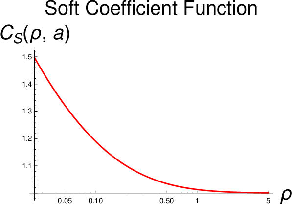
both diverging in the massless limit for the final quark, $\rho\to 0^{+}$ . The complete Soft Coefficient function up to first order,

C_{S}(\rho,a)\,=\,1\,+\,a\,C_{S}^{(1)}(\rho),

(135)

is plotted in fig. 2.

5.3 Soft Remainder Function

The Soft Remainder Function has the usual perturbative expansion beginning at first order:

\mathrm{Rem}_{S}(y;\rho;a)\,=\,a\,\mathrm{Rem}_{S}^{(1)}(y;\rho)\,+\,\mathcal{O}\left(a^{2}\right).

(136)

According to eq.(130), the Soft Remainder Function has the first-order (leading) term given by:

$\displaystyle\mathrm{Rem}_{S}^{(1)}(y;\rho)$	$\displaystyle=$	$\displaystyle E^{(1)}(y;\rho)\,-\,\Sigma_{S}^{(1)}(y;\rho)\,-\,C_{S}^{(1)}(\rho)\,=$	(137)
	$\displaystyle=$	$\displaystyle\big(1\,+\,2\,\rho\big)\bigg\{\frac{1}{2}\Big[\log^{2}(y\,+\,\rho)\,-\,\log^{2}(\rho)\Big]\,+\,\text{Li}_{2}\left(\frac{\rho}{y\,+\,\rho}\right)\,-\,\frac{\pi^{2}}{6}\,+$
		$\displaystyle\qquad\qquad\qquad\qquad\qquad\qquad\qquad-\,\log(y)\Big[\log(y\,+\,\rho)\,-\,\log(\rho)\Big]\bigg\}\,+$
	$\displaystyle+$	$\displaystyle\left(2\,\rho^{3}\,+\,3\,\rho^{2}\,+\,\frac{\rho}{2}\,+\,\frac{1}{4}\right)\Big[\log(y\,+\,\rho)\,-\,\log(\rho)\Big]+$
	$\displaystyle-$	$\displaystyle\frac{y}{y\,+\,\rho}\Bigg\{\rho\left[2\,\rho^{2}\,+\,\rho\,(y\,+\,3)\,-\,\frac{1}{6}\left(2\,y^{2}\,-\,9\,y\,+\,9\right)\right]\,+$
		$\displaystyle\qquad\qquad\qquad\qquad\qquad\qquad\qquad\qquad+\,\frac{y}{12}\left(2\,y^{2}\,-\,3\,y\,-\,30\right)\Bigg\}\,+$
	$\displaystyle+$	$\displaystyle y\left(1\,-\,\frac{y}{4}\right)\Big[\log(1\,+\,\rho)\,-\,\log(y\,+\,\rho)\Big]\,-\,\frac{y}{4\,(y\,+\,\rho)}.$

By taking into account that:

\text{Li}_{2}\left(1\right)\,=\,\sum_{n=1}^{\infty}\frac{1}{n^{2}}\,=\,\frac{\pi^{2}}{6},

(138)

it is immediate to check the vanishing of the Soft Remainder function in the Born kinematics, i.e. in the limit $y\to 0^{+}$ (in taking this limit, $\rho$ is kept constant and not zero: $\rho=\rho_{0}>0$ ). The Soft Remainder Function is plotted in fig. 3 for different values of $\rho$ .

Since

\mathrm{Rem}_{S}^{(1)}(y=1;\,\rho)\,=\,-\,C_{S}^{(1)}(\rho),

(139)

by reducing $\rho$ towards zero (from above, let’s say, from $\rho=1$ ), the corresponding Soft Remainder functions, which are all strictly monotonically decreasing functions, and therefore all negative, become progressively bigger in size.

We can conclude that the Soft Factorization scheme which we have constructed in this section, is very simple, but it only works in the region it is aimed at, namely $y\ll 1$ and $\rho=\mathcal{O}(1)$ : there is no bonus. To consistently describe the small $y$ , small-mass region $\rho\ll 1$ , we have to construct a more general factorization scheme, based on a $QCD$ form factor which also resumes small- $\rho$ effects, i.e. the collinearly enhanced terms.

6 General Factorization

In this section we construct a general factorization scheme, which correctly describes the soft region

0\,<\,y\,\ll\,\rho\,=\,\mathcal{O}(1)\qquad(\mathrm{soft\,\,region})

(140)

and the (effectively) massless region

0\,<\,\rho\,\ll\,y\,\ll\,1\qquad(\mathrm{effectively\,\,massless\,\,region}),

(141)

as well as the ”transition region”

0\,<\,y\,\approx\,\rho\,\ll\,1\qquad(\mathrm{transition\,\,region}).

(142)

As in the previous massless or soft factorization schemes, the factorized event fraction is written as:

E\left(y;\rho;\alpha_{S}\right)\,=\,C\left(\rho;\alpha_{S}\right)\,\Sigma\left(y;\rho;\alpha_{S}\right)\,+\,\mathrm{Rem}\left(y;\rho;\alpha_{S}\right).

(143)

In order to determine the Coefficient function, $C(\rho;\alpha_{S})$ , as well as the Remainder function, $\mathrm{Rem}(y;\rho;\alpha_{S})$ , to $\mathcal{O}\left(\alpha_{S}\right)$ , we need to know the general $QCD$ form factor $\Sigma\left(y;\rho;\alpha_{S}\right)$ , also at first order in the coupling. The latter cannot be evaluated directly, but it can be obtained by expanding in powers of $\alpha_{S}$ the general resummed form factor, as described in the next section.

6.1 General $QCD$ Form Factor

The general $QCD$ form factor, resumming to all orders in $\alpha_{S}$ the infrared (soft and/or collinear) logarithms occurring in the perturbative expansion of the event fraction, has the following expression [18]:

	$\displaystyle\sigma_{N}\left(\rho,\alpha_{S}\right)\,=\,\exp\int\limits_{0}^{1}dy\,\Big[(1-y)^{N-1}\,-\,1\Big]\Bigg\{\frac{1}{y}\int\limits_{Q^{2}y^{2}/(1+\rho)}^{Q^{2}y^{2}/(y+\rho)}\frac{dk_{\perp}^{2}}{k_{\perp}^{2}}\,A\left[\rho;\alpha_{S}\left(k_{\perp}^{2}\right)\right]\,+$		(144)
	$\displaystyle+\,B\left[\alpha_{S}\left(\frac{Q^{2}y^{2}}{y+\rho}\right)\right]\frac{1}{y+\rho}\,+\,D\left[\alpha_{S}\left(\frac{Q^{2}y^{2}}{1+\rho}\right)\right]\frac{1}{y}\,+\,\Delta\left[\alpha_{S}\left(\frac{Q^{2}y^{2}}{1+\rho}\right)\right]\left(\frac{1}{y}\,-\,\frac{1}{y+\rho}\right)\Bigg\}.$

Note that, in the above equation, the term proportional to $\Delta(\alpha_{S})$ describes soft-gluon emission off the strange quark line for $y\raisebox{-3.0pt}{$\>\stackrel{{\scriptstyle<}}{{\scriptstyle\sim}}\>$}\rho$ . As a consequence, this term identically vanishes in the massless limit $\rho\to 0^{+}$ . We may say that the $B$ and $\Delta$ terms are somehow ”complementary”, in the sense that one acts in the kinematic region where the other does not.

Let us remark that the general form factor in eq.(144) reduces to:

1.

the Heavy-to-Light form factor, eq.(84), in the massless limit $\rho\to 0^{+}$ ;
2.

the Soft form factor, eq.(121), in the soft limit $y\to 0^{+}$ , $\rho=$ const $\neq 0$ or, more simply, $y/\rho\to 0^{+}$ .

6.1.1 Form-factor expansion

To compute the partially-integrated form factor $\Sigma=\Sigma(y;\rho;\alpha_{S})$ , expanded up to first order in $\alpha_{S}$ , the only non-trivial integration involved is that one of the term proportional to $a\,A^{(1)}(\rho)$ , namely

\int\limits_{y}^{1}\frac{dy^{\prime}}{y^{\prime}}\,\log\left(\frac{y^{\prime}\,+\,\rho}{1\,+\,\rho}\right).

(145)

In the above expression, the integration of the soft-gluon transverse momentum squared $k_{\perp}^{2}$ has already been made. In order to isolate the large infrared logarithms, the expansion of the resummed form factor is conveniently written — out of the many possible forms — as:

$\displaystyle\Sigma(y;\rho;a)$	$\displaystyle=$	$\displaystyle 1\,+\,a\,A^{(1)}(\rho)\left[-\,\log\left(\frac{y+\rho}{1+\rho}\right)\log(y)\,+\,\frac{1}{2}\,\log^{2}\left(\frac{y+\rho}{1+\rho}\right)\right.+$	(146)
		$\displaystyle\qquad\quad\left.\,+\,\log(1\,+\,\rho)\,\log\left(\frac{y+\rho}{1+\rho}\right)\,+\,\mathrm{Li}_{2}\left(\frac{\rho}{y+\rho}\right)\,-\,\mathrm{Li}_{2}\left(\frac{\rho}{1+\rho}\right)\right]+$
	$\displaystyle+$	$\displaystyle a\,D^{(1)}\,\log(y)\,+\,a\,\Delta^{(1)}\,\left[\log(y)\,-\,\log\left(\frac{y+\rho}{1+\rho}\right)\right]\,+\,a\,B^{(1)}\,\log\left(\frac{y+\rho}{1+\rho}\right)\,+$
		$\displaystyle\qquad\qquad\qquad\qquad\qquad\qquad\qquad\,\,+\,\,\mathcal{O}\left(a^{2}\right).$

The following remarks about the above equation are in order:

1.

Unlike the massless form factor, eq.(80) or (99), a $\log^{2}(y)$ term is absent in eq.(146), because of the regulating effect on collinear emissions of a non-vanishing strange mass, i.e. $\rho\neq 0$ , as discussed in the Introduction. Apart from this term, actually all the possible quadratic and linear terms containing $\log(y)$ and $\log(y+\rho)/(1+\rho)$ do appear in eq.(146);
2.

The arguments of the dilogarithms are always smaller than, or equal to, one, so these term are uniformly bounded by $\mathrm{Li}_{2}(1)=\pi^{2}/6\simeq 1.64493$ — namely a constant of order one.

Checking that the first square bracket on the r.h.s. of eq.(146) is equal to the integral in (145) is quite standard:

1.

One takes the derivatives with respect to $y$ of both expressions and checks that they are equal;
2.

One checks that both expressions are equal for a particular value of $y$ , such as for example the point $y=1$ , where the integral in (145) vanishes.

By replacing the explicit values of the first-order coefficients, one obtains for the first-order form factor,

\Sigma(y;\rho;a)\,=\,1\,+\,a\,\Sigma^{(1)}(y;\rho)\,+\,\mathcal{O}\left(a^{2}\right),

(147)

the explicit expression:

$\displaystyle\Sigma^{(1)}(y;\rho)$	$\displaystyle=$	$\displaystyle\big(1\,+\,2\,\rho\big)\Bigg[-\,\log\left(\frac{y+\rho}{1+\rho}\right)\,\log(y)\,+\,\frac{1}{2}\,\log^{2}\left(\frac{y+\rho}{1+\rho}\right)\,+$	(148)
		$\displaystyle\qquad\qquad\quad\,+\,\log(1\,+\,\rho)\,\log\left(\frac{y+\rho}{1+\rho}\right)+\,\mathrm{Li}_{2}\left(\frac{\rho}{y\,+\,\rho}\right)-\,\mathrm{Li}_{2}\left(\frac{\rho}{1\,+\,\rho}\right)\Bigg]\,+$
		$\displaystyle\,-\,2\log(y)\,+\,\frac{1}{4}\log\left(\frac{y+\rho}{1+\rho}\right).$

The following remarks about the form factor above, eq.(148), are in order:

1.

It reduces to the massless form factor, eq.(80), in the massless limit $\rho\to 0^{+}$ , and to the soft form factor, eq.(127), for $y/\rho\to 0^{+}$ , $\rho\raisebox{-3.0pt}{$\>\stackrel{{\scriptstyle>}}{{\scriptstyle\sim}}\>$}1$ ;
2.

It vanishes in the limit of vanishing photon energy:

$\lim_{y\to 1^{-}}\Sigma^{(1)}(y;\rho)\,=\,0,$ (149)

where one has simply to take into account that

$\lim_{y\to 1^{-}}z(y;\rho)\,=\,1.$ (150)

6.2 General Coefficient function

In order to evaluate the Coefficient and Remainder functions, the first step is to subtract, from the first-order spectrum, eq.(115), the first-order $QCD$ form factor, eq.(148). That way, one obtains:

$\displaystyle C^{(1)}(\rho)\,+\,\mathrm{Rem}^{(1)}(y;\rho)$	$\displaystyle=$	$\displaystyle E^{(1)}(y;\rho)\,-\,\Sigma^{(1)}(y;\rho)\,=$	(151)
	$\displaystyle=$	$\displaystyle\bigg[\rho\left(2\,\rho^{2}\,+\,3\,\rho\,+\,\frac{1}{2}\right)\,-\,y\left(1\,-\,\frac{y}{4}\right)\bigg]\log\left(\frac{y\,+\,\rho}{1\,+\,\rho}\right)\,+$
		$\displaystyle+\,\frac{1\,-\,y}{y\,+\,\rho}\bigg[2\,\rho^{3}\,+\,\rho^{2}(y\,+\,2)\,-\,\frac{\rho}{6}\left(2\,y^{2}\,-\,7\,y\,+\,14\right)\,+$
		$\displaystyle\qquad\qquad\qquad\qquad\qquad\qquad\quad\,+\,\frac{y}{12}\left(2\,y^{2}\,-\,y\,-\,31\right)\bigg].$

The following remarks are in order:

1.

All soft logarithms — namely all $\log(y)$ terms — exactly canceled by subtracting from the spectrum the form factor, as it should, and as already happened in the (simpler) soft factorization scheme. Actually, in the present case, unlike the soft one, the complete cancellation of the first three rows on the r.h.s. of eq.(115) occurred — a large number of terms canceled;
2.

On the last member of eq.(151), the coefficient of the collinear logarithm — namely the term $\log\left[(y+\rho)/(1+\rho)\right]$ — is suppressed by positive powers of $\rho$ or $y$ , again as it should. Note that this did not happen in the soft factorization scheme;
3.

It is immediately checked that the event fraction minus the form factor exactly vanishes at the upper endpoint $y=1$ .

The first-order Coefficient function is given by:

C^{(1)}(\rho)\,=\,\lim_{y\to 0^{+}}\Big[E^{(1)}(y;\rho)\,-\,\Sigma^{(1)}(y;\rho)\Big].

(152)

By taking the above limit, one easily finds:

C^{(1)}(\rho)\,=\,-\,\rho\left(2\,\rho^{2}\,+\,3\,\rho\,+\,\frac{1}{2}\right)\Big[\log(1\,+\,\rho)\,-\,\log(\rho)\Big]\,+\,2\,\rho\,(1\,+\,\rho)\,-\,\frac{7}{3}.

(153)

Unlike the Soft Coefficient function, eq.(132), which, as we have shown, diverges like $\log^{2}(\rho)$ for $\rho\to 0^{+}$ , the general Coefficient function above has a finite value, of order one, in the massless limit:

\lim_{\rho\to 0^{+}}C^{(1)}(\rho)\,=\,-\,\frac{7}{3}.

(154)

Note that the most singular terms for $\rho\to 0^{+}$ in $C^{(1)}(\rho)$ are of the form $\rho\log(\rho)$ (just like the $\mathcal{O}(\alpha_{S})$ correction factor $K(\rho)$ to the inclusive width, see eq.(107)).

The no-recoil limit ( $\rho\to+\infty$ ) of the general Coefficient function does not vanish, but is finite:

\lim_{\rho\to+\infty}C^{(1)}(\rho)\,=\,-\,2.

(155)

Therefore, by increasing $\rho$ from zero to infinity, the first-order coefficient function increases by $1/3$ . A plot of the complete Coefficient function at first order,

C(\rho;a)\,=\,1\,+\,a\,C^{(1)}(\rho),

(156)

as a function of the mass parameter $\rho$ , is given in fig. 4. We observe that $C(\rho;a)$ is basically a monotonically-increasing function of $\rho$ , with a rather mild dependence on this variable. By comparing fig. 4 with fig. 2, we notice a substantial stabilization of the Coefficient function as far as the dependence on $\rho$ is concerned; That is, generically speaking, a ”good new”. Furthermore, while the soft coefficient function is always greater than one, the general coefficient function is always smaller than one.

6.3 General Remainder function

The first-order Remainder function collects, by definition, all the $\mathcal{O}(\alpha_{S})$ terms which are not included neither in the Form Factor nor in the Coefficient function:

\mathrm{Rem}^{(1)}(y;\rho)\,\equiv\,E^{(1)}(y;\rho)\,-\,\Sigma^{(1)}(y;\rho)\,-\,C^{(1)}(\rho).

(157)

By construction (see eq.(152)), it vanishes on Born kinematics:

\lim_{y\to 0^{+}}\mathrm{Rem}^{(1)}(y;\rho)\,=\,0\qquad(\rho=\mathrm{const}>0).

(158)

The first-order Remainder function (the lowest non-vanishing order) explicitly reads:

$\displaystyle\mathrm{Rem}^{(1)}(y;\rho)$	$\displaystyle=$	$\displaystyle\rho\left(2\,\rho^{2}\,+\,3\,\rho\,+\,\frac{1}{2}\right)\log\left(1\,+\,\frac{y}{\rho}\right)\,-\,y\left(1\,-\,\frac{y}{4}\right)\log\left(\frac{y\,+\,\rho}{1\,+\,\rho}\right)\,+$	(159)
	$\displaystyle-$	$\displaystyle 2\,\rho^{2}\,y\,-\,\rho\,y\,(3\,-\,y)\,-\,\frac{y}{6}\left(4\,y^{2}\,-\,9\,y\,-\,9\right)\,+$
	$\displaystyle+$	$\displaystyle\frac{y^{2}}{4\,(y\,+\,\rho)}\left(2\,y^{2}\,-\,5\,y\,+\,4\right)\,-\,\frac{y}{4\,(y\,+\,\rho)}.$

It is immediate to check that the r.h.s. of the above equation vanishes for $y\to 0^{+}$ ( $\rho=\mathrm{const}>0$ ), as all terms are explicitly proportional to $y$ or to higher powers of $y$ , or are proportional to $\log(1+y/\rho)$ , which is also $\mathcal{O}(y)$ .

Note that the second and the third row on the r.h.s. of eq.(159) have been rewritten by means of a partial fractioning with respect to $\rho$ . The general Remainder function is plotted in fig. 5. Similarly to the General Coefficient function, also the General Remainder function has a mild dependence on the mass parameter $\rho$ .

7 Improved Factorization Scheme

In the previous section we have constructed a factorization scheme, given by eqs.(143), (144), (153) and (159), which correctly works in the threshold region $(y\ll 1)$ in the massive case $(\rho\neq 0)$ so long as, in taking the limit $y\to 0^{+}$ , the mass parameter $\rho$ is kept constant and not zero: $\rho=\rho_{0}>0$ . However, it is also natural to ask ourselves what happens if we take the massless limit $\rho\to 0^{+}$ in our massive factorization formula. We have seen that both the massive Coefficient and Remainder functions have a finite limit for $\rho\to 0^{+}$ , while the soft Coefficient and Remainder functions diverge like $\log^{2}(\rho)$ in the same limit. Therefore, as expected, a substantial improvement is obtained by going from the soft factorization scheme to the general one, again as far as the massless limit $\rho\to 0^{+}$ is concerned. The problem then is: by taking the massless limit of our general factorization formula, do we obtain the same Form Factor, the same Coefficient and Remainder functions of the massless factorization scheme, i.e. of the standard factorization scheme applied to the massless event fraction $E_{0}$ , described in sec. 3, or we do not?

Let us begin our analysis by studying the simpler object occurring in the factorization process, namely the Coefficient function. The massless limit in eq.(154),

\lim_{\rho\to 0^{+}}C^{(1)}(\rho)\,=\,-\,\frac{7}{3},

(160)

does not coincide with the massless Coefficient function, i.e. evaluated in the usual factorization of the massless spectrum ( $\rho=0$ from the very beginning: see sec.3):

C_{0}^{(1)}\,=\,\,-\,\frac{31}{12}.

(161)

To obtain the limiting Coefficient function in eq.(160), one has to add to $C_{0}^{(1)}$ the constant $1/4$ :

\lim_{\rho\to 0^{+}}C^{(1)}(\rho)\,=\,C_{0}^{(1)}\,+\,\frac{1}{4}.

(162)

We can say that the following two operations do not commute with each other:³³ 3 Non-commuting phenomena also appear in the factorization of fragmentation functions of heavy quarks [19].

1.

Taking the massless limit $\rho\to 0^{+}$ of the event fraction;
2.

Factorizing the spectrum into a form factor, a coefficient and a remainder functions.

A similar problem, in particular, a ”specular mismatch”, also occurs with the General Remainder function. In the massless limit $\rho\to 0^{+}$ , the general Remainder function becomes:

\lim_{\rho\to 0^{+}}\mathrm{Rem}^{(1)}(y;\rho)\,=\,\,-\,y\left(1\,-\,\frac{y}{4}\right)\log(y)\,-\,\frac{y}{12}\left(2\,y^{2}\,-\,3\,y\,-\,30\right)\,-\,\frac{1}{4}\qquad(y=\mathrm{const}>0).

(163)

The massless limit above does not vanish in the Born-kinematic limit $y\to 0^{+}$ :

\lim_{y\to 0^{+}}\left[\lim_{\rho\to 0^{+}}\mathrm{Rem}^{(1)}(y;\rho)\right]\,=\,-\,\frac{1}{4}.

(164)

Actually, ”symmetrically” with respect to the case of the General Coefficient function, the limiting General Remainder function is equal to the massless one minus the constant $1/4$ :

\lim_{\rho\to 0^{+}}\mathrm{Rem}^{(1)}(y;\rho)\,=\,\mathrm{Rem}_{0}^{(1)}(y)\,-\,\frac{1}{4}.

(165)

By comparing eq.(162) with eq.(165), we find that, by taking the massless limit of the general massive factorization formula, the constant $1/4$ is moved from the Remainder function to the Coefficient function. As already noted, the conclusion is that it makes a difference to take the massless limit $\rho\to 0^{+}$ before Factorization or after Factorization of the spectrum. The problem does not originate from the $QCD$ form factor which, as we have shown, has a smooth behavior in the massless limit $\rho\to 0^{+}$ , so it necessarily originates from the splitting of the non-logarithmic terms between the Coefficient function and the Remainder function.

By looking at the plot of the Remainder function in fig. 5 for $\rho\ll 1$ , one finds a small dip for very small $y$ . The latter is produced by the last term on the r.h.s. of eq.(159), namely the term

-\,\frac{y}{4\,(y\,+\,\rho)}.

(166)

Indeed the dip completely disappears in the subtracted Remainder function,

\overline{\mathrm{Re}}^{(1)}(y;\rho)\,\equiv\,\mathrm{Re}^{(1)}(y;\rho)\,+\,\frac{y}{4\,(y\,+\,\rho)},

(167)

in which the above term has been removed by hand (see fig. 5). Therefore we can conclude that the finite mismatch which we have found, originates from this term only, on which we then focus our attention from now on.

Formally, for any strictly positive (and fixed) value of $\rho$ , whatever small, the ratio (166) vanishes in the threshold limit $y\to 0^{+}$ , so this term is naturally relegated into the massive Remainder function. However for very small values of the mass parameter $\rho$ ,

0\,<\,\rho\,\ll\,1,

(168)

the term (166) is small only in a tiny region of the kinematic variable $y$ , namely the region

0\,<\,y\,\ll\,\rho\qquad(\mathrm{small}\,\,y),

(169)

where:

-\,\frac{y}{4\,(y\,+\,\rho)}\,\approx\,-\,\frac{y}{4\,\rho}\,\ll\,1.

(170)

Therefore only in the small $y$ region (169) (small compared to $\rho$ ), the term in (166) is reasonably inserted into the Remainder function. In the complementary, large $y$ region (again in a strong inequality sense and again compared to $\rho$ ),

0\,<\,\rho\,\ll\,y\qquad(\mathrm{large}\,\,y),

(171)

this term is approximately equal to a constant of order one,

-\,\frac{y}{4\,(y\,+\,\rho)}\,\approx\,-\,\frac{1}{4},

(172)

so it would be reasonable to relegate it inside the Coefficient function, and no more inside the Remainder function.

Mathematically, the problem originates from the fact that:

\lim_{y\to 0^{+}}\,-\,\frac{y}{4\,(y\,+\,\rho)}\,=\,0,

(173)

while:

\lim_{\rho\to 0^{+}}\,-\,\frac{y}{4\,(y\,+\,\rho)}\,=\,-\,\frac{1}{4}.

(174)

The ratio (166) is the only term in the Remainder function, eq.(159), for which the limits $y\to 0^{+}$ and $\rho\to 0^{+}$ do not commute with each other, as:

\lim_{\rho\to 0^{+}}\left[\lim_{y\to 0^{+}}\,-\,\frac{y}{4\,(y\,+\,\rho)}\right]\,=\,\lim_{\rho\to 0^{+}}0\,=\,0;

(175)

while:

\lim_{y\to 0^{+}}\left[\lim_{\rho\to 0^{+}}\,-\,\frac{y}{4\,(y\,+\,\rho)}\right]\,=\,\lim_{y\to 0^{+}}\left(-\,\frac{1}{4}\right)\,=\,-\,\frac{1}{4}\,\neq\,0.

(176)

On the contrary, for the terms of the form $y^{n}/(y+\rho)$ with $n>1$ , appearing on the r.h.s. of eq.(159), the two limits $y\to 0^{+}$ and $\rho\to 0^{+}$ do commute with each other. Note also that more complicated non-commuting terms, such as for example $y^{2}/(y+\rho)^{2}$ or $y^{2}/(y^{2}+\rho^{2})$ , do not appear on the r.h.s. of eq.(159). A crude solution to this problem is to define:

1.

An Improved $(I)$ Coefficient function, by adding to the massive Coefficient function, $C^{(1)}(\rho)$ in eq.(153), the term (166) when the latter is large, i.e. for $y>\rho$ :

$C_{I}^{(1)}(y;\rho)\,\equiv\,C^{(1)}(\rho)\,-\,\frac{y}{4\,(y\,+\,\rho)}\,\theta(y\,-\,\rho);$ (177)

where $\theta(x)\equiv 1$ for $x>0$ and zero otherwise is the standard Heaviside unit step function;

An Improved Remainder function, by adding to the subtracted Remainder function, $\overline{\mathrm{Re}}^{(1)}(y;\rho)$ in eq.(167), the term (166) when the latter is small, i.e. in the complementary case $y<\rho$ :

\mathrm{Re}_{I}^{(1)}(y;\rho)\,\equiv\,\overline{\mathrm{Re}}^{(1)}(y;\rho)\,-\,\frac{y}{4\,(y\,+\,\rho)}\,\theta(\rho\,-\,y).

(178)

Note that:

C_{I}^{(1)}(\rho;y)\,+\,\mathrm{Re}_{I}^{(1)}(y;\rho)\,\equiv\,C^{(1)}(\rho)\,+\,\mathrm{Re}^{(1)}(y;\rho),

(179)

i.e., with the present Improvement, we have simply made a rearrangement of terms among the Coefficient function and the Remainder function. Since the $QCD$ form factor $\Sigma$ equals unity in the free limit,

\Sigma(y;\rho;\alpha_{S})\,=\,1\,+\,\mathcal{O}\left(\alpha_{S}\right),

(180)

it follows that the Improved resummed formula, i.e. eq.(143) with the Improved Coefficient and Remainder functions, coincides with the standard resummed formula or the fixed-order event fraction to $\mathcal{O}\left(\alpha_{S}\right)$ .

An important point is that our improvement necessarily introduces a dependence on $y$ in the massive Coefficient function. In order to have a Coefficient function with a dependence on $y$ which is as simple as possible, one can split the ratio (166) as:

-\,\frac{y}{4\,(y\,+\,\rho)}\,=\,-\,\frac{1}{4}\,+\,\frac{\rho}{4\,(y\,+\,\rho)}.

(181)

When $y>\rho$ , i.e. when the ratio on the l.h.s. above is large, one inserts the constant $-1/4$ inside the Improved Coefficient function, while the (small) fraction $\rho/(4(y\,+\,\rho))$ is inserted in the Improved Remainder function. Therefore one can also define the simpler Improved Coefficient function

C_{I}^{(1)}(y;\rho)\,\equiv\,C^{(1)}(\rho)\,-\,\frac{1}{4}\,\theta(y-\rho);

(182)

together with the Improved Remainder function

\mathrm{Re}^{(1)}_{I}(y;\rho)\,\equiv\,\overline{\mathrm{Re}}^{(1)}(y;\rho)\,-\,\frac{y}{4\,(y\,+\,\rho)}\,\theta(\rho-y)\,+\,\frac{\rho}{4\,(y\,+\,\rho)}\,\theta(y-\rho).

(183)

Let us remark that, even though the non-commuting term (166) is numerically rather small in size, it has its own relevance on the theoretical side. We also expect the presence of similar non-commuting terms to be generic in heavy-to-heavy decays, i.e. not to be restricted to the rare $B\to X_{s}\gamma$ decays. Furthermore, in different processes the size of non-commuting terms can be numerically larger.

7.1 Smoothing the transition

The Improved factorization scheme, which we have constructed in the previous section, can be further improved by eliminating the discontinuities in the Coefficient and Remainder functions produced by the $\theta$ -functions. We can regularize the discontinuities by means of smooth functions with a similar step behavior to the $\theta$ -functions, such as for example the sigmoids (see figs.6 and 7):

\theta(x)\quad\mapsto\quad S_{\Delta}(x)\,\equiv\,\frac{1}{\sqrt{2\pi}\,\Delta}\int\limits_{-\infty}^{x}\exp\left(-\,\frac{t^{2}}{2\,\Delta^{2}}\right)\,dt;

(184)

where $\Delta>0$ is a parameter specifying the size of the $x$ -interval, centered around $x=0$ , where most of the variation of the function $S_{\Delta}(x)$ occurs. It holds indeed:

S_{\Delta}(x=+\Delta)\,-\,S_{\Delta}(x=-\Delta)\,\simeq\,0.68.

(185)

Furthermore, in a weak sense:

\lim_{\Delta\to 0^{+}}\sigma_{\Delta}(x)\,=\,\theta(x),

(186)

so we recover the previous case by sending the auxiliary parameter $\Delta$ to zero. As well known from statistics, $\Delta$ is the standard deviation $\sigma$ of the Gaussian distribution function inside the integral on the r.h.s. of eq.(184).

It is immediate to check the following basic properties of the function $S_{\Delta}(x)$ :

\lim_{x\to-\infty}S_{\Delta}(x)\,=\,0;\qquad\lim_{x\to+\infty}S_{\Delta}(x)\,=\,1;\qquad S_{\Delta}(0)\,=\,\frac{1}{2};\qquad S_{\Delta}(x)\,+\,S_{\Delta}(-x)\,\equiv\,1.

(187)

The smoothed Improved Coefficient and Remainder functions are simply obtained from the previous improved ones, eqs.(182) and (183), by replacing the $\theta$ -functions with $S_{\Delta}$ -functions with the same arguments:

	$\displaystyle C_{I}^{(1)}(y;\rho)$	$\displaystyle\equiv$	$\displaystyle C^{(1)}(\rho)\,-\,\frac{1}{4}\,S_{\Delta}(y-\rho);$
	$\displaystyle\mathrm{Re}_{I}^{(1)}(y;\rho)$	$\displaystyle\equiv$	$\displaystyle\overline{\mathrm{Re}}^{(1)}(y;\rho)\,+\,\frac{\rho}{4\,(y+\rho)}\,S_{\Delta}(y-\rho)\,-\,\frac{y}{4\,(y+\rho)}\,S_{\Delta}(\rho-y).$		(188)

It is natural to assume $\Delta$ to be a function of $\rho$ :

\Delta\,=\,\Delta(\rho),

(189)

together with $\Delta<\rho$ . In practice, for the numerical value of $\Delta$ , one can take a fraction of $\rho$ , such as for example:

\Delta\,=\,\frac{\rho}{3}\quad\mathrm{or}\quad\frac{\rho}{2}.

(190)

7.2 Partition of Unity

One may wish to have an Improved Coefficient function which is as similar as possible to the standard one. Actually, it is possible to construct an Improved Coefficient function which is:

1.

Exactly equal to the massive coefficient function $C^{(1)}(\rho)$ , eq.(153), in the small- $y$ region

$y\,<\,\rho\,-\,\Delta;$ (191)
2.

Independent of $y$ and with the correct massless limit $\rho\to 0^{+}$ , namely $C^{(1)}_{0}$ in eq.(70), in the large- $y$ region

$y\,>\,\rho\,+\,\Delta.$ (192)

This problem can be solved by means of the so-called Partition of Unity, a general analytic method in real geometry [20]. Let us consider the function

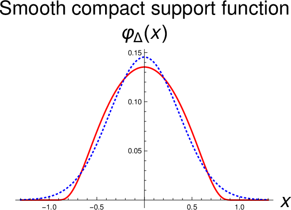
\varphi_{\Delta}(x)\,\equiv\,\exp\left(-\,\frac{1}{\Delta+x}\,-\,\frac{1}{\Delta-x}\right)\qquad\mathrm{for}\,\,\,|x|\,<\,\Delta

(193)

and zero otherwise. In fig. 6 we plot this function for $\Delta=1$ (the red continuous line). Note that the function $\varphi_{1}(x)$ is not qualitatively very different from a Gaussian with standard deviation $\sigma=0.365\approx\Delta/3$ (blue dotted line), even though the latter formally has support on the entire real line.

It is immediate to check that $\varphi_{\Delta}(x)$ is an even function of $x$ ,

\varphi_{\Delta}(-x)\,=\,\varphi_{\Delta}(x).

(194)

By explicitly computing the derivatives of $\varphi_{\Delta}(x)$ of all orders at $x=\pm\Delta$ , it is straightforward to check that this function is infinitely smooth on the real line,

\varphi_{\Delta}\,\in\,C^{\infty}({\mathbb{R}}).

(195)

Given the normalization constant

K\,\equiv\,\int\limits_{-\Delta}^{+\Delta}\varphi_{\Delta}(x)\,dx\,>\,0,

(196)

let us define the function

\Phi_{\Delta}(x)\,\equiv\,\frac{1}{K}\int\limits_{-\infty}^{x}\varphi_{\Delta}(x^{\prime})\,dx^{\prime}.

(197)

Being the primitive of an infinitely smooth function, also $\Phi_{\Delta}$ is a $C^{\infty}({\mathbb{R}})$ function. This function also satisfies the following properties:

1.

It is identically equal to zero for small $x$ , precisely:

$\Phi_{\Delta}(x)\,\equiv\,0\quad\mathrm{for}\,\,x\,<\,-\,\Delta;$ (198)
2.

It is identically equal to one for large $x$ ,

$\Phi_{\Delta}(x)\,\equiv\,1\quad\mathrm{for}\,\,x\,>\,+\,\Delta;$ (199)
3.

It is strictly monotonically increasing in the interval

$-\,\Delta\,<\,x\,<\,+\,\Delta.$ (200)

The function $\Phi_{\Delta}(x)$ is plotted in fig. 7 for $\Delta=1$ .

Note that the function

\Psi_{\Delta}(x)\,\equiv\,\Phi_{\Delta}(x)\,-\,\frac{1}{2}

(201)

is odd in $x$ ,

\Psi_{\Delta}(-x)\,=\,-\,\Psi_{\Delta}(x).

(202)

It vanishes indeed at $x=0$ .

From eq.(202) the fundamental relation follows:

\Phi_{\Delta}(x)\,+\,\Phi_{\Delta}(-x)\,\equiv\,1,\quad x\,\in\,{\mathbb{R}}.

(203)

The required Improved Coefficient and Remainder functions are simply obtained by replacing, inside eqs.(7.1), the $S_{\Delta}$ -functions with $\Phi_{\Delta}$ -functions with the same arguments:

	$\displaystyle C_{I}^{(1)}(y;\rho)$	$\displaystyle\equiv$	$\displaystyle C^{(1)}(\rho)\,-\,\frac{1}{4}\,\Phi_{\Delta}(y\,-\,\rho);$		(204)
	$\displaystyle\mathrm{Re}^{(1)}_{I}(y;\rho)$	$\displaystyle\equiv$	$\displaystyle\overline{\mathrm{Re}}^{(1)}(y;\rho)\,+\,\frac{\rho}{4\,(y\,+\,\rho)}\,\Phi_{\Delta}(y\,-\,\rho)\,-\,\frac{y}{4\,(y\,+\,\rho)}\,\Phi_{\Delta}(\rho\,-\,y).$

The Improved Coefficient function at first order in $a$ (or in $\alpha_{S}$ ),

C_{I}(y;\rho;a)\,=\,1\,+\,a\,C_{I}^{(1)}(y;\rho),

(205)

is plotted in fig. 8.

The Improved Remainder function at first order,

\mathrm{Rem}_{I}(y;\rho;a)\,=\,a\,\mathrm{Rem}_{I}^{(1)}(y;\rho),

(206)

is plotted in fig. 9.

Let’s now prove that the above Improved Coefficient function possesses all the properties we were looking for. When $y<\rho-\Delta$ , the function $\Phi_{\Delta}(y-\rho)$ identically vanishes, so that:

C_{I}^{(1)}(y;\rho)\,\equiv\,C^{(1)}(\rho)\qquad(y\,<\,\rho\,-\,\Delta).

(207)

When $y>\rho+\Delta$ , the function $\Phi_{\Delta}(y-\rho)$ is identically equal to one, so that:

C_{I}^{(1)}(y;\rho)\,\equiv\,C^{(1)}(\rho)\,-\,\frac{1}{4}\qquad(y\,>\,\rho\,+\,\Delta).

(208)

According to eq.(162),

\lim_{\rho\to 0^{+}}C^{(1)}(\rho)\,-\,\frac{1}{4}\,=\,C_{0}^{(1)},

(209)

so that, in the massless limit $\rho\to 0^{+}$ , we recover the coefficient function $C_{0}^{(1)}$ of the standard factorization of the massless spectrum (i.e. the case where the limit $\rho\to 0^{+}$ is taken before the factorization of the perturbative spectrum into a form factor, a coefficient and a remainder functions).

7.3 Generalization

Up to now we have explicitly considered only the contribution of the (leading) operator $O_{7}$ to the radiative $B\to X_{s}\gamma$ decay, contained in the effective non-leptonic weak Hamiltonian (see [12] and references therein)

\mathcal{H}_{eff}\,=\,-\,\frac{4G_{F}}{\sqrt{2}}\lambda_{t}\sum_{j=1}^{8}C_{j}(\mu)O_{j}(\mu).

(210)

$C_{j}(\mu)$ is the Wilson (short-distance) coefficient function of the operator $O_{j}(\mu)$ and $\mu=\mathcal{O}(m_{b})$ is a factorization scale. The operator basis read:

$\displaystyle O_{1}$	$\displaystyle=$	$\displaystyle\bar{c}_{Li}\gamma^{\mu}b_{Lj}\bar{s}_{Lj}\gamma_{\mu}c_{Li};$
$\displaystyle O_{2}$	$\displaystyle=$	$\displaystyle\bar{c}_{Li}\gamma^{\mu}b_{Li}\bar{s}_{Lj}\gamma_{\mu}c_{Lj};$
$\displaystyle O_{3}$	$\displaystyle=$	$\displaystyle\bar{s}_{Li}\gamma^{\mu}b_{Li}\left[\bar{u}_{Lj}\gamma_{\mu}u_{Lj}+\cdots+\bar{b}_{Lj}\gamma_{\mu}b_{Lj}\right];$
$\displaystyle O_{4}$	$\displaystyle=$	$\displaystyle\bar{s}_{Li}\gamma^{\mu}b_{Lj}\left[\bar{u}_{Lj}\gamma_{\mu}u_{Li}+\cdots+\bar{b}_{Lj}\gamma_{\mu}b_{Li}\right];$
$\displaystyle O_{5}$	$\displaystyle=$	$\displaystyle\bar{s}_{Li}\gamma^{\mu}b_{Li}\left[\bar{u}_{Rj}\gamma_{\mu}u_{Rj}+\cdots+\bar{b}_{Rj}\gamma_{\mu}b_{Rj}\right];$
$\displaystyle O_{6}$	$\displaystyle=$	$\displaystyle\bar{s}_{Li}\gamma^{\mu}b_{Lj}\left[\bar{u}_{Rj}\gamma_{\mu}u_{Ri}+\cdots+\bar{b}_{Rj}\gamma_{\mu}b_{Ri}\right];$
$\displaystyle O_{7}$	$\displaystyle\equiv$	$\displaystyle\frac{e}{16\,\pi^{2}}\,\bar{s}_{i}\,\sigma^{\mu\nu}\left(m_{b}\,R\,+\,m_{s}\,L\right)b_{i}\,F_{\mu\nu};$
$\displaystyle O_{8}$	$\displaystyle\equiv$	$\displaystyle\frac{g_{s}}{16\,\pi^{2}}\,\bar{s}_{i}(t^{a})_{ij}\sigma^{\mu\nu}\left(m_{b}\,R\,+\,m_{s}\,L\right)b_{j}\,G_{\mu\nu}^{a};$	(211)

where $i,j=1,2,3$ are color indices (fundamental $SU(3)_{c}$ representation). The operators $O_{1},\cdots,O_{6}$ are 6-dimensional 4-fermion operators, which induce $b\to s$ transitions after contracting the repeated quark fields, such as for example $\bar{c}_{Li}$ and $c_{Li}$ in $O_{1}$ . These contractions therefore generate $b\to s$ effective non-local operators, with photons and/or gluons in the final states attached to the quark loop. Finally $O_{7}/O_{8}$ is a 5-dimensional local magnetic/chromo-magnetic operator.

In this section we generalize the evaluation of the photon spectrum by including all the operators in $\mathcal{H}_{eff}$ . Let us first omit from our computations the operator $O_{8}$ , which has rather peculiar properties to be discussed later.

7.3.1 Massless case

Let us first summarize the results in the simpler massless case ([5] and references therein), in a notation which easily generalizes to the massive case.

Let’s first consider the rare $b$ decay into the simplest final state, namely:

b\,\to\,s\,+\,\gamma.

(212)

At lowest order, $\mathcal{O}(\alpha_{em})$ , only the magnetic operator $O_{7}$ and some 4-fermion operators give a non-zero contribution. An important point is that the effect of these 4-fermion operators can be absorbed into a redefinition of the Wilson coefficient function of $O_{7}$ ([12] and references therein):

C_{7}\quad\mapsto\quad C_{7}^{\mathrm{eff}}\,\equiv\,C_{7}\,+\,e_{d}\,C_{5}\,+\,3\,e_{d}\,C_{6};

(213)

where $e_{d}=-1/3$ is the electric charge of a down-type quark (in units of the proton charge). The lowest-order rate reads:

\Gamma^{(0)}_{77}\,=\,\frac{G_{F}^{2}m_{b}^{5}}{32\,\pi^{3}}\,\big(C_{7}^{\mathrm{eff}}\big)^{2}\,\left|\lambda_{t}\right|^{2}\,\frac{\alpha_{em}}{\pi}.

(214)

Let’s now consider the rare $b$ decay with an additional real gluon in the final state:

b\,\to\,s\,+\,g\,+\,\gamma.

(215)

The second important point is that only the contribution to the rate from $O_{7}$ (schematically, the term $\langle O_{7}\rangle\langle O_{7}\rangle$ ), contains non-integrable infrared singularities. All the other contributions to the partial rate, let’s call them

\Gamma_{ij}^{(1)}(y)\equiv\int\limits_{0}^{y}\frac{d\Gamma_{ij}^{(1)}}{dy^{\prime}}\,dy^{\prime},

(216)

such as for example $\Gamma_{27}^{(1)}(y)$ or $\Gamma_{22}^{(1)}(y)$ , contain integrable infrared singularities or are finite. In other words, $\Gamma_{ij}^{(1)}(y)$ for $(i,j)\neq(7,7)$ does not contain any $\log^{2}y$ and $\log y$ terms without power-suppressed coefficients. Therefore these terms only contribute to the $\mathcal{O}(\alpha_{S})$ Coefficient and Remainder functions in the resummed formulae. The partially integrated rate is then of the form:

	$\displaystyle\int\limits_{0}^{y}\frac{d\Gamma}{dy^{\prime}}(y^{\prime},a)\,dy^{\prime}$	$\displaystyle=$	$\displaystyle\Gamma^{(0)}_{77}\left\{1\,+\,a\,K_{77}^{(1)}\,-\,\frac{a}{2}\,\log^{2}(y)\,-\,a\,\frac{7}{4}\log(y)\,+\,a\,\mathrm{Rem}_{77}^{(1)}(y)+\right.$		(217)
			$\displaystyle\left.\qquad\qquad+\,\sum_{(i,j)\neq(7,7),(8,8)}a\,F_{ij}^{(1)}(y)\right\}\,+\,\mathcal{O}(a^{2});$		(217)

where $K_{77}^{(1)}$ is a constant whose actual value, as we are going to show in a moment, is immaterial, the $O_{7}O_{7}$ -Remainder function $\mathrm{Rem}_{77}^{(1)}(y)$ is the function $H_{0}^{(1)}(y)$ in eq.(73), and

F_{ij}^{(1)}(y)\,\equiv\,\frac{\Gamma_{ij}^{(1)}(y)}{\Gamma^{(0)}_{77}},\qquad(i,j)\,\neq\,(7,7),\,(8,8).

(218)

By defining:

K_{ij}^{(1)}\,\equiv\,F_{ij}^{(1)}(y=0),\qquad(i,j)\,\neq\,(7,7),\,(8,8),

(219)

and

\mathrm{Rem}_{ij}^{(1)}(y)\,\equiv\,F_{ij}^{(1)}(y)\,-\,F_{ij}^{(1)}(0),\qquad(i,j)\,\neq\,(7,7),\,(8,8),

(220)

the partial rate above is rewritten:

	$\displaystyle\int\limits_{0}^{y}\frac{d\Gamma}{dy^{\prime}}(y^{\prime};a)\,dy^{\prime}\,=\,1$	$\displaystyle+$	$\displaystyle a\,\sum_{(i,j)\neq(8,8)}K_{ij}^{(1)}\,-\,\frac{a}{2}\,\log^{2}(y)\,-\,a\,\frac{7}{4}\log(y)\,+$		(221)
		$\displaystyle+$	$\displaystyle a\,\sum_{(i,j)\neq(8,8)}\mathrm{Rem}_{ij}^{(1)}(y).$		(221)

By dividing by the total rate,

\int\limits_{0}^{1}\frac{d\Gamma}{dy}(y;a)\,dy\,=\,1\,+\,a\,\sum_{(i,j)\neq(8,8)}K_{ij}^{(1)}\,+\,a\,\sum_{(i,j)\neq(8,8)}\mathrm{Rem}_{ij}^{(1)}(y=1),

(222)

we obtain the event fraction $E_{0}\equiv E_{m_{s}=0}$ to $\mathcal{O}(\alpha_{S})$ , which is naturally factorized as (compare with eq.(79)):

E_{0}(y;a)\,=\,C_{0}(a)\,\Sigma_{0}(y,a)\,+\,\mathrm{Rem}_{0}(y,a),

(223)

where:

C_{0}(a)\,\equiv\,1\,-\,a\sum_{(i,j)\neq(8,8)}\mathrm{Rem}_{ij}^{(1)}(y=1)\,+\,\mathcal{O}(a^{2}),

(224)

$\Sigma_{0}(y;a)$ is given in eq.(80) and

\mathrm{Rem}_{0}(y,a)\,\equiv\,a\sum_{(i,j)\neq(8,8)}\mathrm{Rem}_{ij}^{(1)}(y)\,+\,\mathcal{O}(a^{2}).

(225)

The following remarks are in order:

1.

All the constants $K_{ij}^{(1)}$ cancel by dividing the partial rate by the total rate;
2.

As far as the dependence on the Wilson coefficient functions is concerned:

$\mathrm{Rem}_{ij}^{(1)}(y)\,\propto\,\frac{C_{i}\,C_{j}}{\big(C_{7}^{\mathrm{eff}}\big)^{2}}.$ (226)

7.3.2 Massive case

Let us now consider the factorization of the photon spectrum in the massive case, $m_{s}\neq 0$ , which is our primary concern. In the massive case, the lowest-order rate gets a correction factor $(1+r)(1-r)^{3}=(1+2\rho)/(1+\rho)^{4}$ , so that:

\Gamma^{(0)}_{77}(\rho)\,=\,\frac{G_{F}^{2}m_{b}^{5}}{32\,\pi^{3}}\,\big(C_{7}^{\mathrm{eff}}\big)^{2}\,\left|\lambda_{t}\right|^{2}\,\frac{\alpha_{em}}{\pi}\frac{1+2\rho}{(1+\rho)^{4}}.

(227)

Since, as far as we know, no analytic expressions of the $\Gamma_{ij}^{(1)}(y,\rho)$ contributions of the photon spectrum are available at present in the massive case, except for $i=j=7$ ⁴⁴ 4 In ref.[11] a one-dimensional integral representation (over the gluon energies) of the contributions to the differential photon spectrum coming from $\langle O_{2}\rangle\langle O_{7}\rangle$ and $\langle O_{2}\rangle\langle O_{2}\rangle$ is given. In this paper it is also shown that the $O_{1}$ contribution vanishes. , let us present a general discussion along the lines of the massless factorization. Similarly to the massless case, the partially integrated rate can be written in the form:

	$\displaystyle\int\limits_{0}^{y}\frac{d\Gamma}{dy^{\prime}}(y^{\prime},\rho,a)\,dy^{\prime}$	$\displaystyle=$	$\displaystyle\Gamma^{(0)}_{77}(\rho)\left\{1\,+\,a\,K_{77}^{(1)}(\rho)\,+\,a\,\Sigma^{(1)}(y,\rho)\,+\,a\,\mathrm{Rem}_{77}^{(1)}(y;\rho)\,+\right.$		(228)
			$\displaystyle\left.\qquad\qquad+\,\sum_{(i,j)\neq(7,7),(8,8)}a\,F_{ij}^{(1)}(y;\rho)\right\}\,+\,\mathcal{O}(a^{2});$		(228)

where $K_{77}^{(1)}(\rho)$ is a $\rho$ -dependent constant, $\Sigma^{(1)}(y,\rho)$ is given in eq.(148), $\mathrm{Rem}_{77}^{(1)}(y;\rho)$ is given in eq.(159) and

F_{ij}^{(1)}(y;\rho)\,\equiv\,\frac{\Gamma_{ij}^{(1)}(y,\rho)}{\Gamma^{(0)}_{77}(\rho)},\qquad(i,j)\,\neq\,(7,7),\,(8,8).

(229)

These quantities have the corresponding massless limits above:

\lim_{\rho\to 0^{+}}K_{77}^{(1)}(\rho)\,=\,K_{77}^{(1)};\qquad\lim_{\rho\to 0^{+}}F_{ij}^{(1)}(y;\rho)\,=\,F_{ij}^{(1)}(y).

(230)

By defining:

K_{ij}^{(1)}(\rho)\,\equiv\,F_{ij}^{(1)}(y=0;\rho)

(231)

and

\mathrm{Rem}_{ij}^{(1)}(y;\rho)\,\equiv\,F_{ij}^{(1)}(y;\rho)\,-\,F_{ij}^{(1)}(y=0;\rho)\qquad(i,j)\,\neq\,(7,7),\,(8,8),

(232)

the partial rate is written:

	$\displaystyle\int\limits_{0}^{y}\frac{d\Gamma}{dy^{\prime}}(y^{\prime},\rho,a)\,dy^{\prime}\,=\,1$	$\displaystyle+$	$\displaystyle a\,\sum_{(i,j)\neq(8,8)}K_{ij}^{(1)}(\rho)\,+\,a\,\Sigma^{(1)}(y,\rho)\,+$		(233)
		$\displaystyle+$	$\displaystyle a\,\sum_{(i,j)\neq(8,8)}\mathrm{Rem}_{ij}^{(1)}(y;\rho)\,+\,\mathcal{O}(a^{2}).$		(233)

7.3.3 General Factorization Scheme

By dividing the partial rate by the total rate, we obtain the event fraction $E$ to $\mathcal{O}(\alpha_{S})$ , which has a general factorization of the form:

E(y;\rho,a)\,=\,C(\rho,a)\,\Sigma(y,\rho,a)\,+\,\mathrm{Rem}(y,\rho,a),

(234)

where:

C(\rho,a)\,\equiv\,1\,-\,a\sum_{(i,j)\neq(8,8)}\mathrm{Rem}_{ij}^{(1)}(y=1;\rho)\,+\,\mathcal{O}(a^{2}),

(235)

$\Sigma(y,\rho,a)$ has been given to $\mathcal{O}(a)$ in eq.(148) and

\mathrm{Rem}(y,\rho,a)\,\equiv\,a\sum_{(i,j)\neq(8,8)}\mathrm{Rem}_{ij}^{(1)}(y;\rho)\,+\,\mathcal{O}(a^{2}).

(236)

7.3.4 Improved Factorization Scheme

Let us now describe the Improved Factorization Scheme in the general case. The terms in the massive Remainder function are naturally decomposed into a commuting piece and a non-commuting one, namely:

\mathrm{Rem}_{ij}^{(1)}(y;\rho)\,=\,L_{ij}^{(1)}(y;\rho)\,+\,N_{ij}^{(1)}(y;\rho),

(237)

where:

\lim_{\rho\to 0^{+}}\left[\lim_{y\to 0^{+}}L_{ij}^{(1)}(y;\rho)\right]\,=\,\lim_{y\to 0^{+}}\left[\lim_{\rho\to 0^{+}}L_{ij}^{(1)}(y;\rho)\right],

(238)

while:

\lim_{\rho\to 0^{+}}\left[\lim_{y\to 0^{+}}N_{ij}^{(1)}(y;\rho)\right]\,\neq\,\lim_{y\to 0^{+}}\left[\lim_{\rho\to 0^{+}}N_{ij}^{(1)}(y;\rho)\right].

(239)

The splitting in eq.(237) can be made on a term-by-term analysis of the Remainder function contributions, either analytically or numerically. The commuting terms do not pose any problem and are treated as in the general factorization scheme above. If $L_{ij}(y=0;\rho)\neq 0$ , this term gives a contribution $L_{ij}(y=0;\rho)$ to the Improved Coefficient function and a contribution $L_{ij}(y;\rho)-L_{ij}(y=0;\rho)$ to the Improved Remainder function.

Let us now consider the (more complicated) non-commuting terms. We can assume that:

\lim_{y\to 0^{+}}N_{ij}^{(1)}(y;\rho)\,=\,0.

(240)

If that is not the case, we impose the above limit by simply subtracting from $N_{ij}^{(1)}(y;\rho)$ its value at $y=0$ :

N_{ij}^{(1)}(y;\rho)\quad\mapsto\quad N_{ij}^{(1)}(y;\rho)\,-\,N_{ij}^{(1)}(0;\rho).

(241)

The constant $N_{ij}^{(1)}(0;\rho)$ is then added back to the commuting contributions (being independent on $y$ , it is trivially a commuting term).

Now the idea is simply to treat the non-commuting terms just like the term $y/(y+\rho)$ above, by means of the Partition of Unity, so that:

The $\mathcal{O}(\alpha_{S})$ Improved Coefficient function is obtained by adding to the General Coefficient function $C^{(1)}(\rho)$ above, eq.(235), the terms $\Phi_{\Delta}(y-\rho)\,N_{ij}^{(1)}(y;\rho)$ , giving:

C_{I}^{(1)}(y;\rho)\,=\,-\,\sum_{(i,j)\neq(8,8)}\mathrm{Rem}_{ij}^{(1)}(y=1;\rho)\,+\,\Phi_{\Delta}(y-\rho)\sum_{(i,j)\neq(8,8)}N_{ij}^{(1)}(y;\rho);

(242)

The $\mathcal{O}(\alpha_{S})$ Improved Remainder function is obtained from the General one, $\mathrm{Rem}^{(1)}(y;\rho)$ in eq.(236), by replacing the non-commuting terms $N_{ij}^{(1)}(y;\rho)$ with the terms $\Phi_{\Delta}(\rho-y)\,N_{ij}^{(1)}(y;\rho)$ respectively, giving:

\mathrm{Rem}_{I}^{(1)}(y;\rho)\,=\,\sum_{(i,j)\neq(8,8)}\left[L_{ij}^{(1)}(y;\rho)\,+\,\Phi_{\Delta}(\rho-y)\,N_{ij}^{(1)}(y;\rho)\right].

(243)

By using eq.(203), it is immediate to check that

\Phi_{\Delta}(y-\rho)\,N_{ij}^{(1)}(y;\rho)\,+\,\Phi_{\Delta}(\rho-y)\,N_{ij}^{(1)}(y;\rho)\,=\,N_{ij}^{(1)}(y;\rho),

(244)

so that the $\mathcal{O}(\alpha_{S})$ event fraction is correctly reproduced.

7.3.5 Alternative formulation

As in the previous explicit computation, the $y$ -dependent contribution to the Improved Coefficient function can be simplified by taking the massless limit $\rho\to 0^{+}$ in $N_{ij}^{(1)}(y;\rho)$ , giving:

C_{I}^{(1)}(y;\rho)\,=\,-\,\sum_{(i,j)\neq(8,8)}\mathrm{Rem}_{ij}^{(1)}(y=1;\rho)\,+\,\Phi_{\Delta}(y-\rho)\sum_{(i,j)\neq(8,8)}N_{ij}^{(1)}(y;\rho=0).

(245)

That generalizes the partial fractioning made in the $O_{7}\,O_{7}$ -case

\frac{y}{y+\rho}\,=\,1\,-\,\frac{\rho}{y+\rho}.

(246)

The Improved Remainder function corresponding to the Improved Coefficient Function given in eq.(245) then reads:

\mathrm{Rem}_{I}^{(1)}(y;\rho)\,=\,\sum_{(i,j)\neq(8,8)}\left[L_{ij}^{(1)}(y;\rho)\,+\,N_{ij}^{(1)}(y;\rho)\,-\,\Phi_{\Delta}(y-\rho)\,N_{ij}^{(1)}(y;\rho=0)\right].

(247)

It is easy to check that also the function on the r.h.s. above vanishes for $y\to 0^{+}$ , as it should. Just remember eq.(240) and the definition of the function $\Phi_{\Delta}(x)$ , eq.(197), together with the fact that $\Delta<\rho$ (note that $N_{ij}^{(1)}(y;\rho=0)$ does not vanish for $y\to 0^{+}$ because of eq.(239)).

7.3.6 Double insertion of $O_{8}$

Let us now consider the effects of the operator $O_{8}$ in the radiative decay $B\to X_{s}\gamma$ . This operator is obtained from $O_{7}$ simply by replacing the electromagnetic field strength $F_{\mu\nu}$ by the $QCD$ one, $G_{\mu\nu}^{a}t^{a}$ , as well as by replacing the electric charge $e$ by the color charge $g_{s}$ ( $\alpha_{em}\equiv e^{2}/(4\pi),\,\,\alpha_{S}\equiv g_{s}^{2}/(4\pi)$ ). As a consequence, the lowest-order matrix element of $O_{8}$ induces the decay

b\,\to\,s\,+\,g.

(248)

Note that the gluon and the strange quark are emitted locally by $O_{8}$ . There are no photons in the final state, which experimentally consists, in the beauty rest frame, of two back-to-back hadronic jets. The topology of the final states in the decay (248) is quite different from that of the tree-level decay mediated by $O_{7}$ ,

b\,\to\,s\,+\,\gamma,

(249)

which consists of one hadronic jet recoiling against a (high-energy) photon.

The lowest-order contribution of $O_{8}$ to the differential photon spectrum is then a spike at vanishing photon energy:

\frac{d\Gamma^{(0)}_{88}}{dx}(x,\rho)\,=\,\Gamma^{(0)}_{88}(\rho)\,\delta(x),

(250)

where:

\Gamma^{(0)}_{88}(\rho)\,=\,\frac{G_{F}^{2}m_{b}^{5}}{32\pi^{3}}\left|C_{8}^{\mathrm{eff}}\lambda_{t}\right|^{2}\frac{C_{F}\alpha_{S}}{\pi}\,\frac{1+2\rho}{(1+\rho)^{4}}.

(251)

$C_{8}^{\mathrm{eff}}$ is an effective (or improved) Wilson coefficient function of $O_{8}$ , including the (non-vanishing) contributions from the 4-fermion operators [12]:

C_{8}^{\mathrm{eff}}\,=\,C_{8}\,+\,C_{5}.

(252)

Note that $\Gamma^{(0)}_{88}(\rho)$ is obtained from $\Gamma^{(0)}_{77}(\rho)$ above simply replacing $C_{7}^{\mathrm{eff}}$ with $C_{8}^{\mathrm{eff}}$ and $\alpha_{em}$ with $C_{F}\alpha_{S}$ .

Let us now consider the $\mathcal{O}(\alpha_{em})$ corrections to the decay (248) involving a real photon, contributing to the process

b\,\to\,s\,+\,g\,+\,\gamma.

(253)

The gluon is again emitted locally by $O_{8}$ , while the photon is emitted by the beauty and the strange quark lines. The contribution to the differential photon spectrum reads [12]:

\frac{1}{\Gamma^{(0)}_{88}}\frac{d\Gamma^{(1R)}_{88}}{dx}\,=\,\frac{\alpha_{em}}{\pi}\,e_{d}^{2}\,X^{(1R)},

(254)

where $e_{d}=-1/3$ and:

	$\displaystyle X^{(1R)}$	$\displaystyle=$	$\displaystyle\frac{1}{2\,(1-r)}\left[\frac{1+(1-x)^{2}}{x}\,+\,r\,\frac{2+x(2-x)}{x}\right]\left[\log\frac{1}{r}\,+\,\log(1-x+r\,x)\right]\,+\qquad$		(255)
		$\displaystyle-$	$\displaystyle\frac{2\,(1-x)}{x}\,+\,\frac{1-r}{4}\left(\frac{1-x}{1-x+rx}\right)^{2}(1-2x)\,-\,\frac{1-r}{4}\frac{1-x}{1-x+rx}\left(1-x+2x^{2}\right).$		(255)

The above spectrum contains a mass singularity of collinear origin for $m_{s}\to 0^{+}$ , as well as a soft singularity for vanishing photon energy ( $x\to 0^{+}$ ):

\frac{1}{\Gamma^{(0)}_{88}}\frac{d\Gamma_{88}^{(R)}}{dx}\,\simeq\,\delta(x)\,+\,e_{d}^{2}\,\frac{\alpha_{em}}{2\pi}\,\hat{P}^{(0)}_{\gamma e}(x)\log\left(\frac{m_{b}^{2}}{m_{s}^{2}}\right)\,-\,e_{d}^{2}\,\frac{\alpha_{em}}{\pi}\,\frac{2}{x},\qquad 0<x,r\ll 1,

(256)

where $\hat{P}^{(0)}_{\gamma e}(x)$ is the leading-order unregularized $QED$ splitting function of an electron (or a positron) into a photon:

\hat{P}^{(0)}_{\gamma e}(x)\,=\,\hat{P}^{(0)}_{ee}(1-x)\,=\,\frac{1+(1-x)^{2}}{x}.

(257)

By coupling the quarks to the electromagnetic field, the strange quark produces a $QED$ jet, as the leading contribution on the r.h.s. of eq.(256) consists of a soft photon emitted at a small angle with respect to the strange quark motion direction. Note that the topology of the $b\to s+g+\gamma$ final states mediated by $O_{8}$ involves two back-to-back jets, initiated by the strange quark and by the gluon. The jet initiated by the strange quark also contains the detected photon. Experimentally, a large hadronic activity around the final photon is then expected. The topology of the $b\to s+g+\gamma$ final states mediated by $O_{7}$ is quite different, as it involves one hadronic jet containing, to $\mathcal{O}(\alpha_{S})$ , the strange quark and the gluon, recoiling against the (hard) photon. In the latter, $O_{7}O_{7}$ -case, the photon is then expected to be isolated.

The r.h.s. of eq.(256) also contains a single-logarithmic term $\propto 1/x$ (upon integration over $x$ ), coming from soft, not collinearly enhanced, radiation off the beauty and the strange quarks (the factor two comes indeed from having two massive quarks in the process). This soft radiation is roughly isotropic in space (in beauty rest frame) and is then not naturally associated to any jet; it represents a kinematic violation of independent jet fragmentation --- the latter coming from angular ordering⁵⁵ 5 Angular ordering is, in turn, an approximate consequence of color coherence — a fundamental dynamical property of perturbative QCD. --- at the next-to-leading level⁶⁶ 6 In process involving light quarks or gluons only, such as for example Drell-Yan production of intermediate vector bosons or Higgs production by gluon-gluon fusion, independent jet fragmentation is instead violated dynamically, usually one order further, i.e. at next-to-next logarithmic accuracy. . As well known, the main effect of the $\mathcal{O}(\alpha_{em})$ virtual corrections to the $O_{8}O_{8}$ tree-level decay, is to introduce a plus regularization in the splitting function and in the soft-singular function, so that:

\frac{1}{\Gamma^{(0)}_{88}}\,\frac{d\Gamma^{(R+V)}}{dx}\,\simeq\,\delta(x)\,+\,e_{d}^{2}\,\frac{\alpha_{em}}{2\pi}\,P^{(0)}_{\gamma e}(x)\log\left(\frac{m_{b}^{2}}{m_{s}^{2}}\right)\,-\,2\,e_{d}^{2}\,\frac{\alpha_{em}}{\pi}\,\left(\frac{1}{x}\right)_{+},

(258)

where:

P^{(0)}_{\gamma e}(x)\,=\,\left[\frac{1+(1-x)^{2}}{x}\right]_{+}\equiv\frac{1+(1-x)^{2}}{x}\,-\,\delta(x)\int\limits_{0}^{1}\frac{1+(1-y)^{2}}{y}\,dy

(259)

and

\left(\frac{1}{x}\right)_{+}\,\equiv\,\frac{1}{x}\,-\,\delta(x)\int\limits_{0}^{1}\frac{dy}{y}.

(260)

By adding virtual photon corrections, soft singularities cancel (in a distribution sense in the differential distribution), while collinear singularities, for $m_{s}\to 0^{+}$ , do not. Therefore one has to factorize the $QED$ collinear logarithm above by means of an ad-hoc fragmentation function, $D_{\gamma s}(x,Q^{2})$ . The latter is a universal, i.e. process-independent, function, which can be interpreted as the probability of finding a photon inside a jet initiated by a strange quark, with a fraction $x$ of the initial strange energy, in a process with hard scale $Q$ ( $Q=m_{b}$ in our case). Since the strange quark mass is of the order of the $QCD$ scale,

m_{s}\,\approx\,\Lambda_{QCD},

(261)

substantial non-perturbative corrections are expected. In order to avoid the introduction of a non-perturbative function — leading in real life to a loss of predictivity — , one can modify the definition of the observed final states, by requiring, for example, the photon to be angularly isolated, in some way, from the final partons/hadrons in the event.

Finally, let us remark that the soft-photon region, $x\ll 1$ , where the operator $O_{8}$ dominates, is experimentally not interesting due to the huge background.

8 Conclusions

We have considered various factorization schemes for threshold resummation in processes involving the decay of a heavy quark into a different heavy (massive) quark, accompanied by non-colored partons, i.e. in practice photons, leptons or vector bosons.

By taking the radiative $B\to X_{s}\gamma$ decay as a model process and restricting ourselves to the leading operator $O_{7}$ in the effective $b\to s\gamma$ weak Hamiltonian, we have first considered soft gluons only and we have constructed a simple soft factorization scheme. The latter can be consistently applied to the heavy quark decays so long as the ordinary velocity of the final quark, in the initial quark rest frame, is not too large (compared to light velocity $c$ ), so that collinear effects (collinear logarithms) are not large. The soft scheme can be probably applied to the CKM-favored semileptonic $B$ decays,

B\,\to\,X_{c}\,+\,l\,+\,\nu_{l},

(262)

as the charm ordinary 3-velocity $v_{c}$ never becomes too large in this case:

v_{c}\,\raisebox{-3.0pt}{$\>\stackrel{{\scriptstyle<}}{{\scriptstyle\sim}}\>$}\,0.77\,c.

(263)

We have then constructed a general massive factorization scheme, which correctly works for a non-zero (and not too small) final quark mass $m_{s}$ . However, we have found that this scheme does not behave well in the massless limit $m_{s}\to 0^{+}$ , because its Coefficient function and its Remainder function do not approach, in this limit, the corresponding functions of the standard factorization formula constructed after taking the massless limit of the photon spectrum. We have shown that this mismatch is generated by a simple term in the photon spectrum (equivalent to the distribution in the final hadron invariant mass squared $m_{X_{s}}^{2}$ ), namely the term, in units of $C_{F}\alpha_{S}/(4\pi)$ ,

\frac{m_{s}^{2}\,-\,m_{X_{s}}^{2}}{m_{X_{s}}^{2}}.

(264)

Indeed, for the above term, the massless limit $m_{s}\to 0^{+}$ and the threshold limit $m_{X_{s}}\to m_{s}^{+}$ do not commute with each other. In terms of the mass-correction parameter $\rho\equiv m_{s}^{2}/(m_{b}^{2}-m_{s}^{2})$ and the threshold variable $y\equiv(m_{X_{s}}^{2}-m_{s}^{2})/(m_{b}^{2}-m_{s}^{2})$ , the above term has been written in the main body of the paper as

-\,\frac{y}{y\,+\,\rho}.

(265)

In the new variables, it is immediate to check that the massless limit $\rho\to 0^{+}$ and the threshold limit $y\to 0^{+}$ do not commute with each other. It is natural to expect the appearance of such terms in the photon spectrum (for which the limits $y\to 0^{+}$ and $\rho\to 0^{+}$ do not commute with each other) to be generic and not restricted to the $O_{7}$ operator. A general discussion of the effects, in the $B\to X_{s}\gamma$ photon spectrum, of all the subleading operators in the effective weak Hamiltonian has also been presented.

Since in semileptonic $b\to c$ decays, eq.(262), the heavy quark mass ratio is rather large, $m_{c}/m_{b}\approx 1/3$ , we expect the general massive scheme to be consistently applied to describe them. We also expect the massive scheme and the soft scheme to give quantitatively similar results for these decays.

Finally, we have constructed an Improved factorization scheme for the massive case, $m_{s}\neq 0$ , which has the correct massless limit $m_{s}\to 0^{+}$ . That is the main result of our work. A main point is that, to that aim, we have been forced to introduce in the Improved Coefficient function $C_{I}$ , in addition to the standard dependence on the mass-correction parameter $\rho$ , also a dependence on the threshold variable $y$ :

C_{I}\,=\,C_{I}(\rho,y).

(266)

Actually, we constructed an Improved Coefficient function which has a smooth dependence both on $y$ and $\rho$ , and which is close to the massless Coefficient function in the quasi-massless region $y\gg\rho$ . The mathematical tool we needed is the so-called Partition of Unity.

By means of the Improved Factorization scheme, it is possible to describe, with a unique formalism and in a smooth way, both the quasi-massless kinematic region $\rho\ll y$ and the pure soft region $y\ll\rho$ , which are dynamically quite different, as well as the transition region $y\approx\rho$ . As is often the case, the interpolation between the asymptotic regions above, to the slice $y\approx\rho$ is, to some extent, arbitrary, as many different functions can be used to that aim. In other words, there is an ambiguity, in the interpolation from the region $\rho\ll y$ to the region $y\ll\rho$ , which is never solved in perturbation theory, but only shifted formally to higher orders.

The improved factorization scheme can be applied, for example, to $CKM$ -favored top quark decays $t\to X_{b}+W$ , in the study of the final hadron invariant squared mass distribution in the intermediate or transition region

m_{X_{b}}^{2}\,-\,m_{b}^{2}\,\approx\,m_{b}^{2}\,\ll\,m_{t}^{2},

(267)

as well as in the soft region

m_{X_{b}}^{2}\,-\,m_{b}^{2}\,\ll\,m_{b}^{2}\,\ll\,m_{t}^{2}

(268)

and in the effectively-massless region

m_{b}^{2}\,\ll\,m_{X_{b}}^{2}\,\ll\,m_{t}^{2}.

(269)

The Improved scheme can also be applied to more complicated decays, such as for example the semileptonic $b\to c$ decay, eq.(262) — a three-body decay at tree level.

We believe that our scheme can be generalized to all the hard processes in which one observes the hadron invariant mass $m_{X}$ of a jet $X$ initiated by a heavy quark $Q$ in all the possible kinematic regions, namely $m_{X}-m_{Q}\ll m_{Q}$ , $m_{X}-m_{Q}\approx m_{Q}$ and $m_{X}\gg m_{Q}$ .

We have explicitly constructed the Improved factorization scheme at order $\alpha_{S}$ , i.e. at Next-to-Leading Logarithmic ( $NLL$ ) accuracy. It would be interesting to explicitly extend the scheme to the next order, i.e. with $\mathcal{O}(\alpha_{S}^{2})$ Coefficient and Remainder functions. The idea of using the Partition of Unity could also be generalized to higher orders.

An extension of our scheme in a different direction could be the construction of an improved factorization formula for resummed transverse momentum distributions involving heavy quarks.

References

[1] U. G. Aglietti, “On the Unsolvability of Bosonic Quantum Fields,” Phil. Mag. 98 (2018) no.35, 3143-3233 doi:10.1080/14786435.2018.1523619 [arXiv:1803.01912 [math-ph]].
[2] J. D. Jackson, “Classical Electrodynamics,” Wiley, 1998, ISBN 978-0-471-30932-1
[3] U. Aglietti, L. Di Giustino, G. Ferrera and L. Trentadue, “Resummed Mass Distribution for Jets Initiated by Massive Quarks”, Phys. Lett. B 651 (2007), 275-292 doi:10.1016/j.physletb.2007.06.034 [arXiv:hep-ph/0612073 [hep-ph]].
[4] See for example: Y. L. Dokshitzer, V. A. Khoze, A. H. Mueller and S. I. Troian, “Basics of perturbative QCD,” Ed. Frontieres (1991), 274 p.
[5] U. Aglietti, “Resummed $B\to X_{u}$ lepton neutrino decay distributions to next-to-leading order,” Nucl. Phys. B 610 (2001), 293-315 doi:10.1016/S0550-3213(01)00316-9 [arXiv:hep-ph/0104020 [hep-ph]].
[6] B. O. Lange, M. Neubert and G. Paz, “Theory of charmless inclusive B decays and the extraction of $V_{ub}$ ”, Phys. Rev. D 72 (2005), 073006 doi:10.1103/PhysRevD.72.073006 [arXiv:hep-ph/0504071 [hep-ph]].
[7] J. R. Andersen and E. Gardi, “Inclusive spectra in charmless semileptonic B decays by dressed gluon exponentiation”, JHEP 01 (2006), 097 doi:10.1088/1126-6708/2006/01/097 [arXiv:hep-ph/0509360 [hep-ph]].
[8] U. Aglietti, G. Ricciardi and G. Ferrera, “Threshold resummed spectra in $B\to X_{u}l\nu$ decays in NLO. I”, Phys. Rev. D 74 (2006), 034004 doi:10.1103/PhysRevD.74.034004 [arXiv:hep-ph/0507285 [hep-ph]].
[9] U. Aglietti, G. Ricciardi and G. Ferrera, “Threshold resummed spectra in $B\to X_{u}l\nu$ decays in NLO (II)”, Phys. Rev. D 74 (2006), 034005 doi:10.1103/PhysRevD.74.034005 [arXiv:hep-ph/0509095 [hep-ph]].
[10] U. Aglietti, G. Ricciardi and G. Ferrera, “Threshold resummed spectra in $B\to X_{u}l\nu$ decays in NLO. III.”, Phys. Rev. D 74 (2006), 034006 doi:10.1103/PhysRevD.74.034006 [arXiv:hep-ph/0509271 [hep-ph]].
[11] A. Ali and C. Greub, “Inclusive photon energy spectrum in rare B decays,” Z. Phys. C 49 (1991), 431-438 doi:10.1007/BF01549696.
[12] A. Ali and C. Greub, “Photon energy spectrum in B — $>$ X(s) + gamma and comparison with data,” Phys. Lett. B 361 (1995), 146-154 doi:10.1016/0370-2693(95)01118-A [arXiv:hep-ph/9506374 [hep-ph]].
[13] J. Kodaira and L. Trentadue, “Soft gluon effects in perturbative Quantum Chromodynamics,” SLAC-PUB-2934.
[14] G. F. Sterman, “Summation of Large Corrections to Short Distance Hadronic Cross-Sections,” Nucl. Phys. B 281 (1987), 310-364 doi:10.1016/0550-3213(87)90258-6
[15] S. Catani and L. Trentadue, “Resummation of the QCD Perturbative Series for Hard Processes,” Nucl. Phys. B 327 (1989), 323-352 doi:10.1016/0550-3213(89)90273-3
[16] G. P. Korchemsky and A. V. Radyushkin, ”Renormalization of the Wilson Loops Beyond the Leading Order”, Nucl. Phys. B 283 (1987), 342-364 doi:10.1016/0550-3213(87)90277-X
[17] See for example: S. Catani, “Soft gluon resummation: A Short review”, [arXiv:hep-ph/9709503 [hep-ph]].
[18] U. Aglietti, L. Di Giustino, G. Ferrera, A. Renzaglia, G. Ricciardi and L. Trentadue, “Threshold Resummation in $B\to X_{c}\,l\,\nu_{l}$ Decays,” Phys. Lett. B 653 (2007), 38-52 doi:10.1016/j.physletb.2007.07.041 [arXiv:0707.2010 [hep-ph]].
[19] D. Gaggero, A. Ghira, S. Marzani and G. Ridolfi, “Soft logarithms in processes with heavy quarks”, JHEP 09 (2022), 058 doi:10.1007/JHEP09(2022)058 [arXiv:2207.13567 [hep-ph]].
[20] See for example: B.A. Dubrovin, A.T. Fomenko and S.P. Novikov, ”Modern Geometry – Methods and Applications, Part II. the Geometry and Topology of Manifolds ”, p. 66, Springer-Verlag New York Inc. (1985).

1 Introduction

2 Phenomenological Relevance

3 Massless Case

3.1 Total decay rate

3.2 Photon spectrum or invariant hadron squared mass distribution

3.3 Factorization

3.4 Threshold resummation in the heavy-to-light case

3.4.1 Form-factor expansion

4 First-order calculation in the massive case

4.1 Total rate

4.2 Photon spectrum

5 Factorization in the Soft limit

5.1 Soft Q​C​DQCD form factor

5.1.1 Form factor expansion

5.2 Soft Coefficient Function

5.3 Soft Remainder Function

6 General Factorization

6.1 General Q​C​DQCD Form Factor

6.1.1 Form-factor expansion

6.2 General Coefficient function

6.3 General Remainder function

7 Improved Factorization Scheme

7.1 Smoothing the transition

7.2 Partition of Unity

7.3 Generalization

7.3.1 Massless case

7.3.2 Massive case

7.3.3 General Factorization Scheme

7.3.4 Improved Factorization Scheme

7.3.5 Alternative formulation

7.3.6 Double insertion of O8O_{8}

8 Conclusions

References

5.1 Soft $QCD$ form factor

6.1 General $QCD$ Form Factor

7.3.6 Double insertion of $O_{8}$