Group Buying Recommendation Model
Based on Multi-task LearningThanks: Corresponding author is Deqing Yang. This work was supported by Shanghai Science and
Technology Innovation Action Plan No.21511100401.
Abstract
In recent years, group buying has become one popular kind of online shopping activities, thanks to its larger sales and lower unit price. Unfortunately, seldom research focuses on the recommendations specifically for group buying by now. Although some recommendation models have been proposed for group recommendation, they can not be directly used to achieve the real-world group buying recommendation, due to the essential difference between group recommendation and group buying recommendation. In this paper, we first formalize the task of group buying recommendation into two sub-tasks. Then, based on our insights into the correlations and interactions between the two sub-tasks, we propose a novel recommendation model for group buying, namely MGBR, which is built mainly with a multi-task learning module. To improve recommendation performance further, we devise some collaborative expert networks and adjusted gates in the multi-task learning module, to promote the information interaction between the two sub-tasks. Furthermore, we propose two auxiliary losses corresponding to the two sub-tasks, to refine the representation learning in our model. Our extensive experiments not only demonstrate that the augmented representations in our model result in better performance than previous recommendation models, but also justify the impacts of the specially designed components in our model. To reproduce our model’s recommendation results conveniently, we have provided our model’s source code and dataset on https://github.com/DeqingYang/MGBR.
Index Terms:
recommendation, group buying, multi-task learning, expert network, gated unitI Introduction
In the last decade, online shopping has become one kind of frequent user activities on Web, and produced great value for many enterprises and society. More recently, more and more users would like to participate in a group buying rather than commit an individual purchase for their favorite products, since one product’s deal price in group buying is generally lower than that in individual purchase.
Besides the deal price, a group buying is essentially different from an individual purchase. We illustrate it with the example in Fig. 1, which comes from the real-world group buying process of online shopping. Fig. 1 (a) depicts the traditional individual purchase, where a user (customer) selects one favorite product from the candidate product list on the e-commerce platform, and directly buys it without considering other customers’ purchases. By contrast, the group buying depicted by Fig. 1 (b) has two phases in fact. In the first phase, a user first selects one favorite product from the candidate list to launch a group for a more lower deal price. Such a user is identified as the initiator of group buying. In the next phase, another user would select one group from the candidate group list, to join it as the role of participant. Each candidate group consists of a product and the corresponding initiator, and may also include other participants who have joined the group before. Thus, there are three types of objects in one group, i.e., initiator, participant and item. A group buying is dealt only when the condition is satisfied, e.g., the number of participants satisfies the preset threshold.
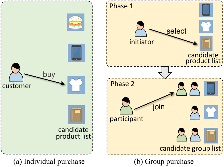
Given the great value of recommender systems in promoting online shopping, the recommendation for group buying deserves being developed. Therefore, we dedicate to propose an effective recommendation model for group buying in this paper, which is seldom studied by previous research of recommendation. Similar to group recommendation [1, 2, 3], there is also a user group consisting of one initiator and some participants in group buying, who interact with the same item. However, the existing models of group recommendation [4, 5, 6, 7] can not be used directly to achieve group buying recommendation due to the following reasons.
1. According to the two phases described in Fig. 1, the recommendation task of group buying addressed in this paper can be divided into two sub-tasks. The first sub-task is to recommend items for a given initiator that he/she would like to launch a group buying. The second sub-task is to recommend participants to join the group given an initiator and the selected item. By contrast, the only task of group recommendation is just to recommend items for a given user group that the users in the group would like to buy. Accordingly, most of the existing group recommendation models mainly focus on how to learn group (preference) representations through aggregating the preferences of group members [8, 4].
2. In addition, unlike group buying, the users in group recommendation do not play different roles of initiator and participant. The previous group recommendation models generally leverage the interactions of group-item-user to learn group representations [7, 4], and some models also leverage the relationships between different groups [6]. Comparatively, the correlations and interactions between initiators, participants and items in group buying are more complicated. It is crucial for group buying modeling to leverage these complicated correlations and interactions sufficiently and correctly.
Therefore, it is challenging to design a recommendation model specifically for group buying. To achieve effective recommendation towards above distinct properties of group buying, we propose a novel recommendation model to accomplish the two sub-tasks of group buying recommendation simultaneously. We denote our model as MGBR (Muti-task learning based Group Buying Recommendation), in which the major multi-task learning module is harnessed to better learn the embeddings of initiators, items and participants. Specifically, based on our insights that the two sub-tasks of group buying recommendation are correlated to each other, we devise some expert networks along with adjusted gates in the multi-task learning module, to promote the information interaction between the two sub-tasks. As a result, the significant information is encoded into the learned embeddings to enhance our model’s recommendation performance. In addition, in order to refine the representation learning in our model, two auxiliary losses corresponding to the two sub-tasks are further proposed to optimize our model training, resulting in more performance gains.
In summary, our contributions in this paper include:
1. We formalize the task of group buying recommendation into two correlated sub-tasks, which indeed conforms to the real-world settings of online shopping. To the best of our knowledge, this is the first to propose a solution of accomplishing these two sub-tasks simultaneously.
2. We propose a novel recommendation model MGBR to achieve the objectives of group buying recommendation, in which we build a multi-task learning module and further devise adjusted gate units, to promote effective information interaction between the two sub-tasks.
3. We further propose two auxiliary learning objectives based on our deep insights into the two sub-tasks of group buying, to refine the representation learning in our model, resulting in further enhanced performance.
4. Our extensive experiments upon a real-world group buying dataset not only demonstrate our model’s advantage over the compared recommendation models, but also justify the impacts of the significant components in our model.
The rest of this paper is organized as follows. In Section II, we first formalize the task of group buying recommendation and then describe our model in detail. Next, we display the experiment results to verify our model’s performance on group buying recommendation in Section III. We introduce the representative works related to our research in Section IV and conclude our work in Section V.
II Methodology
In this section, we first formalize the recommendation task of group buying addressed in this paper, and then detail our proposed recommendation model for group buying.

II-A Task Formalization
At first, we use , , to represent an initiator, item and participant, respectively. According to our description about the group buying process, the two sub-tasks of group buying recommendation can be formalized as follows.
Task A: Recommending an for a given to launch a group buying through computing a scoring function .
Task B: Recommending a for a given pair through computing a scoring function .
As other recommendation models, the recommended objects ( and ) are determined based on the computed and for all items () and participants () in the candidate lists, respectively.
Then, we explain the rationality of computing and to achieve the two sub-tasks of group buying recommendation. Formally, given an observed deal group where is the participant group, a group buying recommendation model should maximize the probability of observing this deal group, that is . In most of group buying’s real scenarios, the participants in one group are not familiar with each other, especially for the deal groups needs hundreds of participants. It indicates that each participant is independent to each other. Thus, we have
Accordingly, the probability and should be maximized by a good recommendation model, which just correspond to (are proportional to) and , respectively.
The training set of our model learning is collected from the observed deal groups. Specifically, for an observed group , is a positive sample of task A. And are the positive samples of task B. For task A and task B, their negative samples are generated through negative sampling, of which the details will be introduced in the following experiment section.
In addition, we denote all user set and item set as and , respectively. Obviously, and . We further use and to denote the positive samples and negative samples of model training, respectively.
II-B Model Overview
We first introduce the pipeline (framework) of our model briefly, as depicted in Fig. 2, which consists of three major steps (modules), i.e., multi-view embedding learning, multi-task learning, and model prediction. At first, in the multi-view embedding learning module, the embeddings of all user (initiators and participants) and items are learned through the graph convolutional networks (GCNs) on three graphs (views) that include different types of connections between initiators, items and participants. The second module is a multi-task learning framework, which is built with some expert networks and gates to exploit the information interaction between the two sub-tasks, since the two sub-tasks are mutually correlated according to the primary principle of group buying. In model prediction module, a multi-layer perceptron (MLP) is built for each sub-task, which is fed with the embeddings output by the gates in the previous module, to computes the score for each candidate item or participant. Furthermore, in order to refine the representation learning of initiators, items and participants in our model, two auxiliary losses are proposed for the two sub-tasks to optimize our model training, resulting in more performance gains.
II-C Multi-view Embedding Learning with GCNs
II-C1 Insights into Object Interactions among Groups
As introduced in Section II-A, our model aims to compute and , which are computed based on the embeddings of the three types of objects, i.e., , and . Thus, learning object embeddings is the preliminary step of our model. According to the positive samples from the observed deal groups, the massive connections (interactions) between the three types of objects are witnessed, based on which the embedding features can be extracted. For example, the user-item interaction graph in many collaborative-filtering (CF) based recommendation models [9, 10] is often leveraged to encode the collaborative signals into the embeddings of users and items, which are significant for the model to generate accurate results. In fact, three undirected graphs can be constructed in our scenario of group buying recommendation, each of which includes two types of objects, i.e., , and . We denote these graphs as , and , and name them as initiator-view, participant-view and social-view, respectively. All of the structural features in , and are significant to learn the embeddings of , and . Given that GCN [11]’s capability of modeling the connections between nodes in a graph, we also apply GCNs on the three graphs to learn their node embeddings. Then, the embeddings of , and are obtained, and therefore we call this step as multi-view embedding learning.
II-C2 Detailed Operations
Specifically, only includes initiator nodes and item nodes. The edge between and is established in if selects to launch a group buying. In fact, is just the user-item interaction graph in task A. Similarly, only includes participant nodes and item nodes, and the edge between and is established if has joined the group buying involving . For , it only has initiator nodes and participant nodes, i.e., only has user nodes. The edge between and is established if has joined the group launched by . Please note that, to save computation costs and reduce connection noises, the edge between any two participants of a group is omitted in 11 1 We have verified that the variant of incorporating the edges between participants even has slightly poor performance.. It is because we believe that in one group the initiator’s preference is more important than other participants’ preferences on learning a participant’s preference, since a participant is often less aware who has also participated in the group. Thus, we learn a participant’s preference from without - edges.
In brief, , and represent distinct connections between . Particularly, user preferences on items can be extracted from and , but they focus on different user roles, i.e., initiator and participant. The preference similarities between users are extracted from , which help the model better recommend participants for a given group.
Formally, suppose , and are the node embedding matrices learned at the -th layer of the GCN on , and , respectively, and is embedding dimension. Then, the computations on the -th layer are as follows,
| (1) |
| (2) |
| (3) |
where , and are the normalized adjacency matrices with self-loops of , and , respectively. And are trainable parameter matrices, is Sigmoid function. Particularly, are randomly initialized by a Gaussian distribution (0, 1).
As shown in Fig. 2, each of has two embeddings of different views through the GCNs on the three views, since each of them is involved in two views. As a result, we directly obtain the multi-view embeddings of as follows,
| (4) |
| (5) |
| (6) |
where is concatenation operator, and are ’s embeddings output by the GCN’s -th layer on and , perspectively. The similar notations are used for and . The learned in this module will be used as the input of the next multi-task learning module.
II-D Multi-task Learning with Expert Networks and Gated Units
II-D1 Insights into Learning Two Sub-tasks
It is reasonable to leverage multi-task learning framework in our model, since the objective of group buying recommendation are divide into task A and task B, as we mentioned before. We should notice that these two sub-tasks are mutual correlated. In task A, user selects item from the candidate item list to launch a group buying, not only based on his/her preference on but also the consideration whether is more favorable among the latent participants. It is up to the specific setting in real-wold group buying. In general, the more latent participants would like to buy , the more likely the group buying of is to be achieved. Recall the example in Fig. 1 (b), the initiator in Phase 1 may like all of the recommended cellphone, T-shirt and book. He would prefer to select the cellphone instead of the book to launch a group buying, if he knows in advance that two participants will follow him to join the group of buying the cellphone in Phase 2, who are more than the followers in other two groups.
Accordingly, our model’s learning of task A requires the intervention of participant information (embeddings) in task B, which encode participants’ preference features. In addition, the learning of task B also needs the information of initiator and item in task A, since the objective of task B is to compute . Notably, each pair in the triple indicates distinct information. Particularly, indicates information of ’s preferences on , which is more focused on by task A. indicates the preference similarity between and , and indicates the information of ’s preference on , both of which are more focused on by task B.
II-D2 Detailed Operations
Inspired by above insights into learning two sub-tasks in group buying recommendation, some information encoded into the object embeddings should be shared sufficiently by task A and task B, to enhance the learning effects of two sub-tasks. Given that the expert network is an effective solution for multi-task learning [12], we also build some expert networks along with gates in this module to achieve learning two sub-tasks, of which the architecture is depicted in Fig. 3. In brief, there are three sub-modules in our multi-task learning module, which correspond to the learning of task A, task B and shared information (denoted as S), respectively. For each sub-module, expert networks collaborate with one gate to learn object embeddings.
For clear statement, we use to denote the three sub-modules, and distinguish their corresponding notations. Formally, suppose is the output embedding of the -th expert network A at layer , and computed as
| (7) |
where are the output embeddings of gate A and gate S at layer , respectively, and is a trainable weight matrix.
Similarly, we also compute the output embedding of the -th expert network B at layer as
| (8) |
where is the output embedding of gate B at layer , and is a trainable weight matrix.
For the output embedding of the -th expert network S at layer , which should involve gate A and gate B besides gate S. Thus, we have
| (9) |
where is also a trainable weight matrix.
Next, we introduce how to compute the output embeddings of all gates mentioned in Eq. 7 9 as follows.
To fully reflect the insights introduced in Section II-D1, we append the adjusted gated unit for gate A, B and S, besides the generic gated unit, which follows the principle of self-attention in [13]. According to this principle, the embeddings learned by the gate are the attentive aggregation of the embeddings learned by expert network A, B and S. Specifically, the output embedding of each gate consists of two sections.
For gate A, the first section of output embedding at layer is calculated through the following generic gated operations as
| (10) | ||||
where is the input embedding of expert network A at layer , and is a trainable weight matrix. Eq. 10 implies that the information of is extracted from the expert network at layer in terms of the information in the previous layer.
Furthermore, the second section of gate A’s output embedding at layer is calculated as
| (11) |
where are both trainable weight matrices, and . Eq. 11 implies that the information of is also extracted from the expert network at layer but in terms of the input ’s information. In addition, the output embeddings of expert network A interact with instead of and , because task A focuses more on the information of . Meanwhile, the information from and are transferred through expert network S.
Then, the overall output embedding of gate A at layer is
| (12) |
where is a control coefficient.
Similarly, the output embedding of gate B is calculated as
| (13) | ||||
Compared with and , the computation of is not so complicate, which is calculated as
| (14) |
where is also a trainable weight matrix.
In addition, to compute we set
| (15) |
which are just the inputs of the expert networks at the first layer, and also the inputs of the multi-task learning module. Accordingly, the weight matrices in the first layer of expert networks have different sizes to that in other layers, i.e., .
II-E Prediction Module
In this module, our model predicts and respectively with the output embeddings of gate A and gate B at the final layer (layer ) respectively. As we introduced before, the two scores are used to achieve the two sub-tasks in group buying recommendation, and computed as
| (16) |
| (17) |
where represents the operations of MLP fed with the output embedding of gate A/B at the last layer. represents the operations of our multi-task learning module. Then, the candidate item with the largest is taken as the recommendation result of task A. Similarly, the candidate participant with the largest is taken as the recommendation result of task B.
Please note that, the in Eq. 16 is obtained by a different way of that in Eq. 17. In task A, all users except for are the potential participants for the group buying of . Thus, we average the embeddings of all users as the in Eq. 16. By contrast, in task B, the in Eq. 17 is just the embedding of the candidate participant who needs being judged by the model.
II-F Model Optimization
In fact, the recommendation task of our work is also the ranking-based recommendation of implicit feedback [14, 15, 9, 16, 17]. Thus, for both of the two sub-tasks in our model, we use the Bayesian ranking loss (BPR) [18] as the objectives of our model optimization. Specifically, the overall loss of our model learning is as follows,
| (18) |
and
| (19) |
where is the control coefficient (weight) of , () denotes the positive (negative) training samples of task A/B. We adopt negative sampling to collect the negative samples in our training set, which will be detailed in the subsequent experiment section.
In addition, we adopt Adam [19] as the optimization method to train our model.
II-G Refining Representation Learning with Auxiliary Losses
Based on our insights into the two sub-tasks of group buying recommendation, we further propose two auxiliary losses for our model training to refine the representation (object embedding) learning in our model. These auxiliary losses’ effects on enhancing recommendation performance are verified by our experiments.
II-G1 Task A’s Auxiliary Loss
Although the information of the participants in task B would influence task A, according to our aforementioned analysis, in task A the model should pay more attention to the match between and , rather than the match between and . It is because that the preference on is the primary reason for to launch a group buying with . Another merit of such consideration is to avoid introducing more noise from the potential participants into task A learning. It implies that, for a positive (observed) triple from historical group buying records, replacing with other items degrades the model’s prediction score more than replacing with other users. Accordingly, our model should try to ensure
| (20) | |||
where is computed as in Eq. 16 except that is just the embedding of the participant . () is the corrupted item (participant) not existing in the true group buying records.
To propose the auxiliary loss for task A, for a given triple in the positive samples of task A’s training set, we first define and where is the set of all participants who have joined the group including and . In our experiments, we set and of any to the same fixed size, denoted as , through negative sampling.
Besides BPR loss, the ListNet loss [20] is also a list-wise loss appropriate for ranking-based recommendation. Thus, based on above idea, we propose the following auxiliary loss of task A as
| (21) | ||||
where if triple , otherwise . In fact, Eq. 21 is proposed to fine-tune the embeddings of , of which the idea is similar to contrastive learning [21].
II-G2 Task B’s Auxiliary Loss
The consideration of refining representation learning in task B is different to that in task A. On the one hand, replacing with other item in a true triple should degrade the model’s prediction score apparently, since can not attract the participant to join the group due to the mismatch between ’s preference on . On the other hand, replacing with other user in a true triple should also degrade the model’s prediction score apparently, still due to the mismatch between ’s preference on . Accordingly, our model should try to ensure
| (22) |
and
| (23) |
In fact, encouraging Eq. 23 is just the objective of task B, which has been reflected by the loss of Eq. 19. Thus encouraging Eq. 22 can be regarded as the auxiliary objective of task B. Given that Eq. 22 is also a form of pair ranking, we implement it also by a BPR-based loss as
| (24) |
Then, the overall loss of our model in Eq. 18 is modified as
| (25) |
where are also the control coefficients of auxiliary losses.
II-H Time Complexity Analysis
Given that we build multiple layers consisting of expert networks and gates in the multi-task learning module of MGBR, to achieve complicated information interaction between sub-module A, B and S, MGBR’s time consumption is undoubtedly bigger than the recommendation models only with GCNs and the matrix factorization (MF) based models. We mainly analyze the time complexity of MGBR’s multi-task learning module as follows, and display the empirical results of comparing the time consumption of MGBR and other models in the subsequent experiment section.
At first, the time complexity of multi-view embedding learning is . Then, we analyze the time complexity of processing a sample in MGBR’s multi-task learning module. For one layer consisting of expert networks and one gate, one expert consumes the time of , hence experts consume . In the adjusted gate unit, the time complexity of computing in Eq. 10 is . And the time complexity of computing in Eq. 11 is . So it consumes to obtain . Similarly, the calculation of and is also . Thus, the time complexity of layers in the multi-task learning module is . Given that and are generally small number, the time consumption of the multi-task learning module is approximate to , i.e., the square of embedding dimension, which is affordable.
III Experiments
In this section, we conduct extensive experiments on one real-world dataset of group buying to answer the following research questions:
- •
RQ1: Does our proposed recommendation model perform better than previous models on the recommendation of group buying?
- •
RQ2: Can the specifically designed components of our model contribute to the performance improvement of group buying recommendation?
- •
RQ3: How do the hyper-parameters of our model affect the performance of group buying recommendation?
III-A Experiment Data
III-A1 Dataset of Group Buying
By now, seldom group buying datasets from the real-world e-commerce platforms are available. The datasets used in the previous group recommendation models [4, 5, 6] can not be used to evaluate our task of group buying, due to the essential difference between them that we have mentioned in Section I. In our experiments, we used a public group buying dataset extracted from Beibei22 2 https://github.com/Sweetnow/group-buying-recommendation [22] to evaluate all compared models. Beibei is the largest e-commerce platform in China for maternal and infant products. This dataset contains the logs of sufficient group buying records, from which the initiator, product and participants of each deal group can be identified. Furthermore, two users (either an initiator or a participant) in a deal group of training set are recognized as a pair of social friends.
Although we only used this one dataset for our evaluations which only includes the products of maternal and infant, we believe that the evaluation results can justify our model’s feasibility to other group buying scenarios, since the group buying on other e-commerce platforms has the same (or very similar) properties as that of Beibei.
| Object | Number |
|---|---|
| user | 125,012 |
| item | 30,516 |
| deal group | 430,360 |
III-A2 Sample Collection
Before collecting the samples of our training and test set, we first filtered out the users who have less than five purchase records in the original Beibei dataset, which follows the popular manipulation in previous work [18, 16]. Then, we removed each group including the filtered users (no matter initiator or participant) and used the rest dataset in our experiment. The statistics of our preprocessed dataset is listed in Table I.
The training and test samples of task A and task B were collected as follows. Each pair and triple observed from any dealt group in the processed dataset are used as one positive sample of task A and task B, respectively. Then, for any initiator of a group, we randomly selected a product (negative item) from the products that has not bought, to accompany as a negative sample of task A. For an observed deal group where is the participant set, we randomly selected a user (negative participant) from to accompany as a negative sample of task B. The ratio of positive samples to negative samples is 1:9. Accordingly, for each test instance in task A () and each test instance in task B (), the sizes of their candidate lists are both 10. The model should compute the score for each item/participant in the candidate list, based on which each test instance’s ranking list is determined. In addition, the ratio of training, validation and test set is 7:3:1.
III-B Baselines
We compared our model with the following recommendation models in our experiments to answer RQ1. In fact, all baselines can achieve the recommendation task of group buying through appropriate tailor although none of them were proposed specially for the two sub-tasks in this paper.
DeepMF [23]: It is a deep version of MF-based recommendation model, in which the rows and columns of user-item interaction matrix are input into multi-layer non-linear projection neural networks, to learn the latent representations of users and items.
NGCF [10]: It is a deep CF model with GCNs, which explicitly models higher order connectivity between user-item interactions to improve embedding representations.
DiffNet [24]: We believe that the social-based recommendation models enhancing user preference modeling with social links can also achieve the recommendation task of group buying, since we regard the relationships between initiators and participants as social links. Thus we also included social-based recommendation models into our comparisons. DiffNet is a representative social recommendation model with GCNs. It utilizes social relations and stimulates the social diffusion process on social networks for better representation learning of users and items. We consider this recommendation model in our comparisons due to that, the co-occurrence relationships between users observed from historical purchase records can be recognized as social links that are crucial for group buying recommendation.
EATNN [25]: It is also a social-aware recommendation model that uses attention mechanisms to automatically assign personalized migration solutions to users by taking into account both their preferences on items and social relationships.
GBGCN [22]: It is in fact one of group recommendation models. Although this model was proposed specifically for group buying and also distinguishes the roles of initiator and participant, it only achieves task A according to our task formalization. In this model, both user-item interaction graph and user-user social graph are constructed to learn the embeddings of users and items. An embedding propagation network is leveraged to extract user preferences in different roles.
GBMF [22]: It was proposed as the variant of GBGCN, which directly uses dot-based similarity function to calculate scores of candidate items and candidate users as MF-based recommendation models. It also updates the embeddings of users and items for better performances.
We explain how to tailor these baselines to simultaneously achieve the two sub-tasks of group buying recommendation as our model. At first, task A can regarded as general item recommendation, all baselines can achieve it directly. Although all baselines were not designed specifically for task B, we can tailor them to achieve task B, only through altering their prediction layers and without modifying their major frameworks. In fact, the representations (embeddings) of are both learned in all of the baselines. According to their modeling principle, either embedding of has encoded the significant information from the rest two objects. Given that task B is similar to user recommendation [26, 27, 28], i.e., for a given user () recommending another user () who has the same/similar preference as and would like to join ’s group, we can directly use the distance of ’s embedding and ’s embedding as . Specifically, we used inner product of two embeddings to measure their distance, since it is widely used in many recommendation models [14, 10, 9].
In addition, we propose the following ablated variants of our MGBR to answer RQ2.
MGBR-M: In this variant, the shared information of multi-task learning framework is removed from our model. In other words, expert network S and gate S are both removed, making our model degrade into a two-tower model over the three views.
MGBR-R: In this variant, we remove the auxiliary loss and in our model training.
MGBR-M-R: In this variant, the shared information in the multi-task learning framework, as well as the two auxiliary losses are both removed.
MGBR-G: This variant replaces the adjusted gated units with generic gated units, indicating that in Eq. 12 and in Eq. 13 are both removed. In other words, .
MGBR-D: In this variant, the three divided views are replaced with an overall heterogeneous information network (HIN) including all nodes of and their relations. The embeddings of are learned by the GCN over this big HIN.
| Para. | Value | Comment |
|---|---|---|
| 128 | embedding dimension | |
| 2 | the number of GCN layers | |
| 6 | the number of expert networks in each layer | |
| 2 | the layer number of expert networks and gates | |
| 99 | negative sampling size in the auxiliary losses | |
| 0.1 | control coefficient of Eq. 12 | |
| 0.1 | control coefficient of Eq. 13 | |
| 1 | control coefficient of in Eq. 25 | |
| 0.3 | control coefficient of in Eq. 25 | |
| 0.3 | control coefficient of in Eq. 25 | |
| 0.0002 | learning rate | |
| 64 | batch size |
| Task A | Task B | |||||||
|---|---|---|---|---|---|---|---|---|
| 1:9 | 1:99 | 1:9 | 1:99 | |||||
| MRR@10 | NDCG@10 | MRR@100 | NDCG@100 | MRR@10 | NDCG@10 | MRR@100 | NDCG@100 | |
| DeepMF | 0.3763 | 0.5183 | 0.1672 | 0.3046 | 0.3070 | 0.4656 | 0.0654 | 0.2209 |
| NGCF | 0.5607 | 0.6617 | 0.2841 | 0.4150 | 0.3778 | 0.5211 | 0.1254 | 0.2748 |
| DiffNet | 0.3780 | 0.5206 | 0.1290 | 0.2771 | 0.3314 | 0.4844 | 0.0976 | 0.2483 |
| EATNN | 0.5827 | 0.6807 | 0.2240 | 0.3736 | 0.3404 | 0.4929 | 0.0727 | 0.2310 |
| GBGCN | 0.5095 | 0.6231 | 0.2775 | 0.4006 | 0.3668 | 0.5127 | 0.1168 | 0.2665 |
| GBMF | 0.3718 | 0.5135 | 0.1433 | 0.2867 | 0.3254 | 0.4794 | 0.0884 | 0.2406 |
| MGBR | 0.6401 | 0.7292 | 0.2876 | 0.4501 | 0.6484 | 0.7327 | 0.2877 | 0.4471 |
| Improvement | 9.85% | 7.13% | 1.23% | 8.46% | 71.65% | 40.61% | 129.43% | 62.70% |
III-C Implementation Details
All of our experiments were conducted on the workstations of GeForce RTX 3090 with 24G memory and the environment of Ubuntu18.04.5 and torch1.8.0. The hyper-parameter settings of all baselines for the following displayed results were decided based on our tuning studies. For our MGBR, some hyper-parameters’ optimal values in the subsequent experiments are listed in Table II, wherein the tuning study results of will be displayed afterwards.
III-D Evaluation Protocols
In our experiments, We adopted MRR@N (mean reciprocal rank) and NDCG@N (normalized discounted cumulative gain) [15, 17] to evaluate all models’ recommendation performance, since they are very popular to evaluate ranking-based recommendation. Particularly, NDCG is more sensitive than MRR to the positive item/participant’s position in the ranking list. f About the ratio of positive sample to negative sample in the test set, we also adopted 1:9 to compute MRR/NDCG@10, and further adopted 1:99 to compute MRR/NDCG@100 for all compared models.
| Task A | ||||||||
| 1:9 | 1:99 | |||||||
| MRR@10 | R. Drop | NDCG@10 | R. Drop | MRR@100 | R. Drop | NDCG@100 | R. Drop | |
| MGBR-M-R | 0.2531 | -152.90% | 0.4327 | -68.5% | 0.0809 | -255.5% | 0.2571 | -75.1% |
| MGBR-M | 0.2607 | -145.53% | 0.4401 | -65.7% | 0.1217 | -136.3% | 0.3095 | -45.4% |
| MGBR-G | 0.6126 | -4.49% | 0.7041 | -3.56% | 0.2732 | -5.27% | 0.4322 | -4.14% |
| MGBR-R | 0.4228 | -51.40% | 0.5663 | -28.77% | 0.1221 | -135.54% | 0.3136 | -43.53% |
| MGBR-D | 0.5189 | -23.36% | 0.6390 | -14.12% | 0.2091 | -37.54% | 0.3793 | -18.67% |
| MGBR | 0.6401 | – | 0.7292 | – | 0.2876 | – | 0.4501 | – |
| Task B | ||||||||
| MGBR-M-R | 0.2344 | -176.62% | 0.4141 | -76.9% | 0.1043 | -175.8% | 0.2946 | -51.8% |
| MGBR-M | 0.2471 | -162.40% | 0.4272 | -71.5% | 0.1147 | -150.8% | 0.3051 | -46.5% |
| MGBR-G | 0.4707 | -37.75% | 0.6001 | -22.10% | 0.1797 | -60.10% | 0.3448 | -29.67% |
| MGBR-R | 0.4769 | -35.96% | 0.6074 | -20.63% | 0.1661 | -73.21% | 0.3437 | -30.08% |
| MGBR-D | 0.4494 | -44.28% | 0.5858 | -25.08% | 0.1501 | -91.67% | 0.3301 | -35.44% |
| MGBR | 0.6484 | – | 0.7327 | – | 0.2877 | – | 0.4471 | – |
III-E Overall Performance Comparisons
The performances scores of all compared models on the two sub-tasks are listed in Table III, where the best scores are bold. As well, the relative performance improvements between our MGBR and the strongest baselines (highlighted with underline) are also displayed. All reported performance scores of each model are the average results of three runnings. Based on these results, we have the following observations and analyses.
1. Obviously, our MGBR has the best performance in both of the two sub-tasks, which should be attributed to several factors. At first, thanks to the GCNs on the multiple views, MGBR can extract rich significant features from the correlations between initiators, items and participants. Second, the significant information is shared by the two sub-tasks in the multi-task learning module. Furthermore, the auxiliary losses help our model promote information interactions and reduce conflicts between the two sub-tasks. It is no surprise that our MGBR outperforms the baselines in task B more apparently than in task A, since none of the baselines are designed for task B. In addition, MGBR leverages the information of the given and more sufficiently to predict in task B.
2. Our MGBR outperforms GBGCN and GBMF on the two sub-tasks, although these two baselines were also proposed for group buying. Compared with GBMF, GBGCN has better performance and further utilizes the features from the heterogeneous graph of initiators, items and participants, which also verifies the advantage of introducing graph structural feature and GCNs.
3. DiffNet performs poorly, although it has excellent performance in social recommendation. The reason may be that the co-occurrence relationships of users in the same groups are not real social relationships, that only reflect the common preferences of users. Comparatively, EATNN performs better than DiffNet in Task A, but it is still inferior to our MGBR.
4. The power of GCN is the major reason of NGCF’s superior performance over other baselines. In addition, unlike DiffNet and GBGCN, it has no special design for capturing social context, avoiding the influence of fake social relationships in the dataset.
5. All baselines fail to obtain satisfactory performance in task B, although all of them were trained on both task A and task B simultaneously. It implies that the training for task B is more difficult and worthwhile to be explored further. It is also necessary to design specific module for task B in general recommendation models.
III-F Ablation Study
We also compared our MGBR with its ablated variants to answer RQ2. All compared variants’ performance scores and their relative performance drops compared with MGBR are listed in Table IV, based on which we have the following observations and analyses.
1. MGBR’s performance improvements over MGBR-M are more than that over MGBR-R and MGBR-G, showing that the shared expert networks and gates (S) are more significant than the auxiliary losses and adjusted gated units on improving our model’s performance.
2. MGBR’s superiority over MGBR-R, and MGBR-M’s superiority over MGBR-M-R both justify the effectiveness of refining representation learning with the auxiliary losses.
3. MGBR-G’s performance drop relatively to MGBR on task B is more prominent than on task A. It is because task B is indeed more difficult, since it requires models to capture not only users’ personalized preferences, but also the common preferences among different users. The adjusted gates in MGBR was proposed to better achieve to the multi-task learning including the auxiliary learning objectives, which leverages prior experiences () to assign appropriate weights to different experts. Compared with task B, task A is less sensitive to the choice of experts since it is more simple.
4. MGBR-D is also inferior to MGBR, showing that including all user and item nodes, along with their relations into an HIN can not obtain the optimal node embeddings through the GCN over the HIN. In fact, the divided views in MGBR can effectively alleviate the negative interactive effects between different relations.
| Model | Para. number | Min./epoch |
|---|---|---|
| DeepMF | 155,500 | 0.34 |
| NGCF | 9,962,176 | 3.17 |
| DiffNet | 15,556,217 | 1.67 |
| EATNN | 33,966,534 | 1.23 |
| GBGCN | 15,555,273 | 1.79 |
| GBMF | 1,555,280 | 1.03 |
| MGBR | 31,341,038 | 8.35 |
III-G Model Scale and Efficiency Comparisons
Table V lists the scale of model parameters and the time consumption (minutes) of one training epoch for all compared models. As we mentioned before, our MGBR is the most time-consuming as it has more complex architecture (more parameters) than the baselines. In EATNN, each user is represented by three kinds of embeddings, so it even has more parameters than our MGBR due to its great number of users. However, it only adopts attentions and MLP operations which are relatively simple compared with MGBR’s architecture, thus consumes less time.
III-H Influence of Important Hyper-parameters
To answer RQ3, we also investigated the influence of some important hyper-parameters of our model on recommendation performance.
III-H1 Impact of Auxiliary Loss Weight
The ablation studies have verified that the two auxiliary losses, i.e., and are helpful for our model to obtain improved performance. To analyze the influence of the weight of and we set in Eq. 25 and set their values in the range of {0.1, 0.2, 0.3, 0.4, 0.5}, and recorded the corresponding recommendation performance comparison on the two sub-tasks as shown in Fig. 4. According to the tuning results, MGBR performs the best when . It shows that either lower or higher value of and would hurt model performance. Too small and make it difficult to constrain our model with the auxiliary losses and reduce the model’s generalization. While too large and would cause our model to overlook fitting with the observed group buying records.
III-H2 Impact of Control Coefficient in Adjusted Gate
To analyze the influence of the control coefficient in the adjusted gates, we also set in Eq. 12 the same as in Eq. 13, and varied their values in the range of {0.05, 0.1, 0.2, 0.3}. Our model’s performance corresponding to these values are displayed in Fig. 5, showing that is the optimal setting for our model to achieve the best performance. The large and indicate that the gate information is extracted in terms of the information of more than the expert networks, resulting in the insufficient utilization of expert network’s information. The small and result in the insufficient utilization of ’s information, and also hurt the model’s performance.

5

III-I Case Study of Representation Learning
As other recommendation models, the representation learning of initiators, items and participants is the key of our model to achieve the task of group buying recommendation. Optimal object embeddings in the model evidently result in better recommendation performance. In this subsection, we visualize the effectiveness of the shared information (expert network and gate S) in our multi-task learning module and the auxiliary losses on refining the object embeddings through some cases.

To this end, we applied PCA decomposition to project all object embeddings into a 2-D space. Fig. 6 displays the embeddings of some groups in MGBR-M-R (a) and MGBR (b), where the colors indicate different groups. The stars, plusses and dots represent the embeddings of initiators, items and participants, respectively. From the figure, we observe that the users and items of the same group (the same color) in MGBR are more concentrated than that in MGBR-M-R, and the embeddings of different groups are distinguishable. It shows that, with the shared information in the multi-task learning module and auxiliary losses, our model is capable of leveraging the information interactions within one group to learn better object embeddings, and thus improves recommendation performance.
IV Related Work
IV-A Recommender Systems
IV-A1 Item Recommendation
Item recommendation [29] aims to predict the probability of a user interacting with a candidate item, and then recommend the item with the highest probability from the candidate set to the user. In recent years, many deep recommendation models [14, 23, 15, 17] have been proposed. Besides leveraging user-item interactions to infer the relationships between user and items, some literatures have introduced social context into item recommendation, based on the assumption that a user has the same or similar preference as his/her friends. Jamali et al. [26] introduced social relations in MF [30] to make the representations of social friends more close, to enhance recommendation performance. [31] recommends items for users through combining a user’s preference and his friends’ preferences. In addition, [24] uses the propagation of user embedding on social networks to capture social influences, and [25] adopts attention mechanisms to automatically assign personalized migration solutions to users by considering both their preferences on items and social relationships.
IV-A2 User Recommendation
Besides item recommendation, user recommendation [28, 27] is another popular scheme in recommender systems, which generally predicts the probability of the interaction between two users. Traditional user recommendation task is just a binary classification to judge whether a candidate user deserves to be recommended to the target user. The second sub-task in our group buying recommendation is in fact a user recommendation task, but the given object is an item and an initiator instead of a sole user. The classical recommendation methods such as MF can also be used to achieve user recommendation. For example, SocialMF [26] adds trust propagation to MF, so as to improve recommendation performance. SocialReg [32] uses two kinds of social information to design social regularization terms to constraint matrix decomposition objective function. Besides the social links between users [33], other features about user preferences can also be leveraged in promote recommendation performance, including user tags [34], activities [27], etc.
IV-A3 Group Recommendation
Although there is essential difference between group recommendation [1, 3] and group buying recommendation, group recommendation is still the recommendation category most related to group buying recommendation. The key problems to achieve group recommendation include how to fuse the preference of each user in a group into the group’s preference [2], and how to handle the disagreements among group members [1]. The classical approaches include [8, 35, 36]. Cao et al. [4] used attention mechanism to learn precious user and group interest representations. Since the social relationships among users indicate their preference similarities, many group recommendation models leverage social information to learn the group representations [7, 37, 38, 39]. Specifically, GBGCN [22] was proposed to capture structural information among group buying records, and model user dual role, social influence and complex group buying implicit feedback. Although it also focuses on group buying, it still aims to solve the first sub-task, i.e., recommending items to a given group as other group recommendation models. For occasional group recommendation, GroupSA [40] models the group decision making process as multiple voting processes, and uses a stacked social self-attention network to simulate how a group consensus is reached. In addition, the knowledge graph (KG) is also helpful to learning group representations [5]. Besides online shopping, group recommendation is also applied in many other areas, such as POI recommendation [41] and restaurant recommendation [42].
IV-A4 Graph Neural Networks for Recommendation
Graph neural networks (GNNs) can capture structural features of graphs via message passing between the nodes, which have been widely used in recommender systems. For example, GNN is used in the matrix completion task for recommendation [43]. NGCF [10] uses embedding propagation on the bipartite graph to model high-order collaborative signals. In addition, GNNs have been successfully employ in session-based recommendation. Wu et al. [44] used GNNs to capture item relation between different sessions and in knowledge-based recommendation. KGAT [45] harnesses graph attention network (GAT) [46] to obtain more accurate and sufficient feature representations. Meng et al. [47] leveraged GGNN [48] to capture the complex patterns among the items in a session.
IV-B Multi-task Learning
Multi-task learning (MTL) helps recommender systems achieve better recommendation through leveraging the information from different aspects, which has been widely incorporated into many recommender systems [47]. A classical MTL approach is hard-parameter sharing, forcing different tasks to share the same parameters. For example, [49] uses the shared-bottom structure to make all tasks share the bottom layer parameters. In industry, ESSM [50] achieves CTR and CVR tasks simultaneously, and generates outstanding results on large-scale data. Similarly, [51] adds a counterfactual learning task to ESSM to alleviate sample selection bias (SSB), and thus achieves better performance on industrial data.
Comparatively, soft-parameter sharing only requires to share a part of the parameters rather. Specifically, it allows each task to select a sub-network, reducing the impact of correlation between tasks. [51, 52] take mixture-of-expert as an important component of MTL, employing different experts to learn different aspects of the features. [12] proposes the idea of multi-gate, that makes it possible for expert networks to pass different information to different tasks. Ma et al. [53] proposed a more flexible soft-parameter sharing approach to add parameter sharing process inside the shared layers, and make the information propagation between expert networks trainable. [13] explicitly divides the expert networks into task-share and task-specific parts, and replaces the fully connected propagation between expert layers with the propagation between the two parts. Accordingly, the MTL of our MGBR also belongs to soft-parameter sharing.
More recently, more flexible and robust MTL approaches have been proposed. For example, AITM [54] takes the sequential relationship into account and uses an information migration module to model task dependencies. In this way, information migration occurs not only at the bottom layers, but also at the layers close to the output. [55] introduces contrastive learning [21] to alleviate the parameter conflict problem in MTL. Sun et al. [56] proposed the sparse-sharing approaches, in which the parameters are partially shared across tasks, making it more flexible to handle loosely related tasks.
V Conclusion
In this paper, we pioneer the task formalization of group buying recommendation for the online shopping platforms. Aiming to achieve the two sub-tasks of group buying recommendation simultaneously, we propose a novel recommendation model MGBR. Based on our insights into the correlations and information interaction between the two sub-tasks, we design collaborative expert networks and adjusted gated units in MGBR’s multi-task learning module, to better learn the object embeddings in buying groups. Furthermore, we propose two auxiliary losses corresponding to the two sub-tasks for model training, to refine representation learning. Our extensive experiments evidently justify MGBR’s superior performance of group buying recommendation over the previous recommendation models.
References
- [1] S. Amer-Yahia, S. B. Roy, A. Chawla, G. Das, and C. Yu, “Group recommendation: Semantics and efficiency,” Proc. VLDB Endow., vol. 2, no. 1, pp. 754–765, 2009.
- [2] S. B. Roy, L. V. S. Lakshmanan, and R. Liu, “From group recommendations to group formation,” in Proceedings of the 2015 ACM SIGMOD International Conference on Management of Data. ACM, 2015, pp. 1603–1616.
- [3] “Group recommendations,” in Encyclopedia of Social Network Analysis and Mining, 2nd Edition, R. Alhajj and J. G. Rokne, Eds. Springer, 2018.
- [4] D. Cao, X. He, L. Miao, Y. An, C. Yang, and R. Hong, “Attentive group recommendation,” in The 41st International ACM SIGIR Conference on Research & Development in Information Retrieval, SIGIRs. ACM, 2018, pp. 645–654.
- [5] Z. Deng, C. Li, S. Liu, W. Ali, and J. Shao, “Knowledge-aware group representation learning for group recommendation,” in 37th IEEE International Conference on Data Engineering, ICDE 2021, Chania, Greece, April 19-22, 2021. IEEE, 2021, pp. 1571–1582.
- [6] L. Guo, H. Yin, T. Chen, X. Zhang, and K. Zheng, “Hierarchical hyperedge embedding-based representation learning for group recommendation,” ACM Trans. Inf. Syst., vol. 40, no. 1, pp. 3:1–3:27, 2022.
- [7] M. Gartrell, X. Xing, Q. Lv, A. Beach, R. Han, S. Mishra, and K. Seada, “Enhancing group recommendation by incorporating social relationship interactions,” in Proceedings of the 2010 International ACM SIGGROUP Conference on Supporting Group Work, GROUP 2010. ACM, 2010, pp. 97–106.
- [8] L. Baltrunas, T. Makcinskas, and F. Ricci, “Group recommendations with rank aggregation and collaborative filtering,” in Proceedings of the 2010 ACM Conference on Recommender Systems, 2010, pp. 119–126.
- [9] X. He, K. Deng, X. Wang, Y. Li, Y. Zhang, and M. Wang, “Lightgcn: Simplifying and powering graph convolution network for recommendation,” in Proceedings of the 43rd International ACM SIGIR conference on research and development in Information Retrieval, Virtual Event, China, July 25-30, 2020. ACM, 2020, pp. 639–648.
- [10] X. Wang, X. He, M. Wang, F. Feng, and T.-S. Chua, “Neural graph collaborative filtering,” in Proceedings of the 42nd international ACM SIGIR conference on Research and development in Information Retrieval, 2019, pp. 165–174.
- [11] T. N. Kipf and M. Welling, “Semi-supervised classification with graph convolutional networks,” in 5th International Conference on Learning Representations, ICLR 2017, Toulon, France, April 24-26, 2017, Conference Track Proceedings. OpenReview.net, 2017.
- [12] J. Ma, Z. Zhao, X. Yi, J. Chen, L. Hong, and E. H. Chi, “Modeling task relationships in multi-task learning with multi-gate mixture-of-experts,” in Proceedings of the 24th ACM SIGKDD international conference on knowledge discovery & data mining, 2018, pp. 1930–1939.
- [13] H. Tang, J. Liu, M. Zhao, and X. Gong, “Progressive layered extraction (ple): A novel multi-task learning (mtl) model for personalized recommendations,” in Fourteenth ACM Conference on Recommender Systems, 2020, pp. 269–278.
- [14] X. He, L. Liao, H. Zhang, L. Nie, X. Hu, and T.-S. Chua, “Neural collaborative filtering,” in Proceedings of the 26th international conference on World Wide Web, 2017, pp. 173–182.
- [15] D. Yang, Z. Guo, Z. Wang, J. Jiang, Y. Xiao, and W. Wang, “A knowledge-enhanced deep recommendation framework incorporating gan-based models,” in IEEE International Conference on Data Mining, ICDM 2018, Singapore, November 17-20, 2018. IEEE Computer Society, 2018, pp. 1368–1373.
- [16] X. He, H. Zhang, M. Kan, and T. Chua, “Fast matrix factorization for online recommendation with implicit feedback,” in Proceedings of the 39th International ACM SIGIR conference on Research and Development in Information Retrieval, SIGIR 2016. ACM, 2016, pp. 549–558.
- [17] D. Yang, C. Shen, B. Liu, L. Xue, and Y. Xiao, “Generating knowledge-based attentive user representations for sparse interaction recommendation,” IEEE Trans. Knowl. Data Eng., vol. 34, no. 9, pp. 4270–4284, 2022.
- [18] S. Rendle, C. Freudenthaler, Z. Gantner, and L. Schmidt-Thieme, “BPR: bayesian personalized ranking from implicit feedback,” in UAI 2009, Proceedings of the Twenty-Fifth Conference on Uncertainty in Artificial Intelligence. AUAI Press, 2009, pp. 452–461.
- [19] D. P. Kingma and J. Ba, “Adam: A method for stochastic optimization,” in 3rd International Conference on Learning Representations, ICLR 2015, San Diego, CA, USA, May 7-9, 2015, Conference Track Proceedings, 2015.
- [20] Z. Cao, T. Qin, T.-Y. Liu, M.-F. Tsai, and H. Li, “Learning to rank: from pairwise approach to listwise approach,” in Proceedings of the 24th international conference on Machine learning, 2007, pp. 129–136.
- [21] A. van den Oord, Y. Li, and O. Vinyals, “Representation learning with contrastive predictive coding,” CoRR, vol. abs/1807.03748, 2018.
- [22] J. Zhang, C. Gao, D. Jin, and Y. Li, “Group-buying recommendation for social e-commerce,” in 2021 IEEE 37th International Conference on Data Engineering (ICDE). IEEE, 2021, pp. 1536–1547.
- [23] H. Xue, X. Dai, J. Zhang, S. Huang, and J. Chen, “Deep matrix factorization models for recommender systems,” in Proceedings of the Twenty-Sixth International Joint Conference on Artificial Intelligence, IJCAI 2017, Melbourne, Australia, August 19-25, 2017. ijcai.org, 2017, pp. 3203–3209.
- [24] L. Wu, P. Sun, Y. Fu, R. Hong, X. Wang, and M. Wang, “A neural influence diffusion model for social recommendation,” in Proceedings of the 42nd International ACM SIGIR Conference on Research and Development in Information Retrieval, SIGIR 2019, Paris, France, July 21-25, 2019. ACM, 2019, pp. 235–244.
- [25] C. Chen, M. Zhang, C. Wang, W. Ma, M. Li, Y. Liu, and S. Ma, “An efficient adaptive transfer neural network for social-aware recommendation,” in Proceedings of the 42nd International ACM SIGIR Conference on Research and Development in Information Retrieval. ACM, 2019, pp. 225–234.
- [26] M. Jamali and M. Ester, “A matrix factorization technique with trust propagation for recommendation in social networks,” in Proceedings of the fourth ACM conference on Recommender systems, 2010, pp. 135–142.
- [27] C. Dai, F. Qian, W. Jiang, Z. Wang, and Z. Wu, “A personalized recommendation system for netease dating site,” Proc. VLDB Endow., vol. 7, no. 13, pp. 1760–1765, 2014.
- [28] S. Kutty, R. Nayak, and L. Chen, “A people-to-people matching system using graph mining techniques,” World Wide Web, vol. 17, no. 3, pp. 311–349, 2014.
- [29] B. Sarwar, G. Karypis, J. Konstan, and J. Riedl, “Item-based collaborative filtering recommendation algorithms,” in Proceedings of the 10th international conference on World Wide Web, 2001, pp. 285–295.
- [30] Y. Koren, R. Bell, and C. Volinsky, “Matrix factorization techniques for recommender systems,” Computer, vol. 42, no. 8, pp. 30–37, 2009.
- [31] A. Davoudi, “Effects of user interactions on online social recommender systems,” in 33rd IEEE International Conference on Data Engineering, San Diego, CA, USA, April 19-22, 2017. IEEE Computer Society, 2017, pp. 1444–1448.
- [32] H. Ma, D. Zhou, C. Liu, M. R. Lyu, and I. King, “Recommender systems with social regularization,” in Proceedings of the fourth ACM international conference on Web search and data mining, 2011, pp. 287–296.
- [33] S. Kim, “Friend recommendation with a target user in social networking services,” in 31st IEEE International Conference on Data Engineering Workshops, ICDE Workshops 2015. IEEE Computer Society, 2015, pp. 235–239.
- [34] D. Yang, L. Chen, J. Liang, Y. Xiao, and W. Wang, “Social tag embedding for the recommendation with sparse user-item interactions,” in IEEE/ACM International Conference on Advances in Social Networks Analysis and Mining. IEEE Computer Society, 2018, pp. 127–134.
- [35] Q. Yuan, G. Cong, and C.-Y. Lin, “COM: a generative model for group recommendation,” in The 20th ACM SIGKDD International Conference on Knowledge Discovery and Data Mining. ACM, 2014, pp. 163–172.
- [36] E. Quintarelli, E. Rabosio, and L. Tanca, “Recommending new items to ephemeral groups using contextual user influence,” in Proceedings of the 10th ACM Conference on Recommender Systems, 2016, pp. 285–292.
- [37] H. Yin, Q. Wang, K. Zheng, Z. Li, J. Yang, and X. Zhou, “Social influence-based group representation learning for group recommendation,” in 2019 IEEE 35th International Conference on Data Engineering (ICDE). IEEE, 2019, pp. 566–577.
- [38] “Social-enhanced attentive group recommendation,” IEEE Trans. Knowl. Data Eng., vol. 33, no. 3, pp. 1195–1209, 2021.
- [39] P. Wang, L. Li, R. Wang, G. Xu, and J. Zhang, “Socially-driven multi-interaction attentive group representation learning for group recommendation,” Pattern Recognit. Lett., vol. 145, pp. 74–80, 2021.
- [40] L. Guo, H. Yin, Q. Wang, B. Cui, Z. Huang, and L. Cui, “Group recommendation with latent voting mechanism,” in 36th IEEE International Conference on Data Engineering, ICDE 2020, Dallas, TX, USA, April 20-24, 2020. IEEE, 2020, pp. 121–132.
- [41] Q. Zhu, S. Wang, B. Cheng, Q. Sun, F. Yang, and R. N. Chang, “Context-aware group recommendation for point-of-interests,” IEEE Access, vol. 6, pp. 12 129–12 144, 2018.
- [42] Q. Zhu and L. Wang, “Context-aware restaurant recommendation for group of people,” in 2020 IEEE World Congress on Services (SERVICES). IEEE, 2020, pp. 51–54.
- [43] R. van den Berg, T. N. Kipf, and M. Welling, “Graph convolutional matrix completion,” CoRR, vol. abs/1706.02263, 2017.
- [44] S. Wu, Y. Tang, Y. Zhu, L. Wang, X. Xie, and T. Tan, “Session-based recommendation with graph neural networks,” in Proceedings of the AAAI Conference on Artificial Intelligence, vol. 33, no. 01, 2019, pp. 346–353.
- [45] X. Wang, X. He, Y. Cao, M. Liu, and T.-S. Chua, “Kgat: Knowledge graph attention network for recommendation,” in Proceedings of the 25th ACM SIGKDD International Conference on Knowledge Discovery & Data Mining, 2019, pp. 950–958.
- [46] P. Velickovic, G. Cucurull, A. Casanova, A. Romero, P. Liò, and Y. Bengio, “Graph attention networks,” in 6th International Conference on Learning Representations, ICLR, Vancouver, BC, Canada, Conference Track Proceedings. OpenReview.net, 2018.
- [47] W. Meng, D. Yang, and Y. Xiao, “Incorporating user micro-behaviors and item knowledge into multi-task learning for session-based recommendation,” in Proceedings of the 43rd International ACM SIGIR conference on research and development in Information Retrieval, SIGIR 2020, Virtual Event, China, July 25-30, 2020. ACM, 2020, pp. 1091–1100.
- [48] Y. Li, D. Tarlow, M. Brockschmidt, and R. S. Zemel, “Gated graph sequence neural networks,” in 4th International Conference on Learning Representations, ICLR 2016, San Juan, Puerto Rico, May 2-4, 2016, Conference Track Proceedings, 2016.
- [49] R. Caruana, “Multitask learning,” Machine learning, vol. 28, no. 1, pp. 41–75, 1997.
- [50] X. Ma, L. Zhao, G. Huang, Z. Wang, Z. Hu, X. Zhu, and K. Gai, “Entire space multi-task model: An effective approach for estimating post-click conversion rate,” in The 41st International ACM SIGIR Conference on Research & Development in Information Retrieval, 2018, pp. 1137–1140.
- [51] H. Wang, T. Chang, T. Liu, J. Huang, Z. Chen, C. Yu, R. Li, and W. Chu, “ESCM2: entire space counterfactual multi-task model for post-click conversion rate estimation,” pp. 363–372, 2022.
- [52] N. Shazeer, A. Mirhoseini, K. Maziarz, A. Davis, Q. V. Le, G. E. Hinton, and J. Dean, “Outrageously large neural networks: The sparsely-gated mixture-of-experts layer,” 2017.
- [53] J. Ma, Z. Zhao, J. Chen, A. Li, L. Hong, and E. H. Chi, “Snr: Sub-network routing for flexible parameter sharing in multi-task learning,” in Proceedings of the AAAI Conference on Artificial Intelligence, vol. 33, no. 01, 2019, pp. 216–223.
- [54] D. Xi, Z. Chen, P. Yan, Y. Zhang, Y. Zhu, F. Zhuang, and Y. Chen, “Modeling the sequential dependence among audience multi-step conversions with multi-task learning in targeted display advertising,” in Proceedings of the 27th ACM SIGKDD Conference on Knowledge Discovery & Data Mining, 2021, pp. 3745–3755.
- [55] D. Zou, W. Wei, X. Mao, Z. Wang, M. Qiu, F. Zhu, and X. Cao, “Multi-level cross-view contrastive learning for knowledge-aware recommender system,” pp. 1358–1368, 2022.
- [56] T. Sun, Y. Shao, X. Li, P. Liu, H. Yan, X. Qiu, and X. Huang, “Learning sparse sharing architectures for multiple tasks,” in Proceedings of the AAAI Conference on Artificial Intelligence, vol. 34, no. 05, 2020, pp. 8936–8943.