Secure Distributed Gram Matrix Multiplication
Abstract
The Gram matrix of a matrix is defined as (or ). Computing the Gram matrix is an important operation in many applications, such as linear regression with the least squares method, where the explicit solution formula includes the Gram matrix of the data matrix. Secure distributed matrix multiplication (SDMM) can be used to compute the product of two matrices using the help of worker servers. If a Gram matrix were computed using SDMM, the data matrix would need to be encoded twice, which causes an unnecessary overhead in the communication cost. We propose a new scheme for this purpose called secure distributed Gram matrix multiplication (SDGMM). It can leverage the advantages of computing a Gram matrix instead of a regular matrix product.
I Introduction
Secure distributed matrix multiplication (SDMM) has been used to compute the product of two matrices using the help of worker servers, while keeping the matrices information-theoretically secure against colluding workers. SDMM was first introduced by Chang and Tandon in [1]. Many different schemes have since been presented, such as the secure MatDot scheme in [2], the GASP scheme in [3] and the DFT scheme in [4]. These schemes compute the products over finite fields, but computations over complex numbers have also been considered in [5, 6, 7]. Other secure coded computation tasks have also been considered, such as batch matrix multiplication in [8, 9], arbitrary polynomial evaluation using Lagrange coded computation in [10], and convolution in [11].
In this paper we will consider the computation of the Gram matrix for some matrix . In general, the Gram matrix is defined using some inner product. We want to consider this multiplication also over finite fields, where the concept of inner product is not meaningful. Hence, we only consider the product . Such a computation is an important step in many applications. For example, if is a matrix representing centered data of variables and observations, then an estimate of the covariance matrix can be computed by . Another example is linear regression using the least squares method, where the aim is to solve the following minimization problem
for some given data matrix and a vector . If the rows of are linearly independent, then the solution obtains the explicit form
Here, computing the Gram matrix of is only one step in the whole computation. However, if is a matrix, where , then inverting the matrix is less computationally heavy than computing the Gram matrix .
The Gram matrix of the matrix can be computed more efficiently compared to regular matrix multiplication of the matrices and . The Gram matrix is symmetric, which means that only the lower (or upper) triangular part needs to be computed and stored as the other half can be obtained by symmetry. For more efficient algorithms on Gram matrix multiplication, see [12].
A Gram matrix can easily be computed using SDMM by considering the matrix multiplication of and . However, this would not be particularly efficient, since it would involve encoding the matrix essentially twice. As communication cost is an important consideration, it is valuable to find even small decreases in the upload cost. Additionally, the multiplication performed by the workers can not utilize the benefits of Gram matrix multiplication, since the results will not be symmetric in general. This leads us to study some variants of standard SDMM schemes, which can be utilized to compute the Gram matrix efficiently. The idea is to encode the matrix just once, such that the computational task of the workers consists of computing the Gram matrix of the encoded pieces. This approach requires a nontrivial choice of the linear code, so that the product can be obtained from these partial results.
Our proposed methods will be based on degree tables, which were first introduced in [13]. However, we consider symmetric degree tables, which have not been studied previously to our knowledge. The Gram matrix multiplication has also been considered in [10] with the Lagrange coded computation scheme, but the scheme was not optimized for this specific problem. We also present an analog version of the scheme, which has much lower communication cost, but is not able to provide security.
II Preliminaries
We write and . Unless mentioned otherwise, we consider matrices and scalars over a finite field with elements. The group of units of is denoted by . Vectors in are considered to be row vectors. If is a matrix, then and denote the submatrices with the first rows and the the rest of the rows, respectively. Furthermore, if is a set of indices, then is the submatrix of with the columns indexed by .
The key tool in distributed coded computation is partitioning the task into smaller subtasks. For matrices this is achieved by partitioning the matrix into equal sized block matrices. One common partitioning is the inner product partitioning (IPP), where the matrices and are partitioned such that
Then their product can be expressed as . Another partitioning is the outer product partitioning (OPP), where the matrices and are partitioned such that
Then their product can be expressed as
The aim of distributed matrix multiplication is to partition the computation into smaller subcomputations, which can be distributed to the worker servers. Secure distributed matrix multiplication puts an additional constraint, which states that no information about the original matrices should be leaked during this process. Most SDMM schemes in the literature follow some kind of linear structure, where the encoded matrices are obtained as linear combinations of the matrices and some random noise that is added. This structure has been presented as a general framework called linear SDMM in [14]. We shall present our contributions using the help of this framework.
A linear SDMM model with workers and colluding workers follows the steps below.
- •
Partitioning the matrices and into and equal sized pieces, respectively.
- •
Computing the encodings
where the matrices and are chosen uniformly at random. Here are generator matrices of some linear codes.
- •
Worker computes the product and returns it to the user.
- •
The user recovers the product by computing some linear combinations of the responses .
The recovery threshold of an SDMM scheme is the minimal number of responses the user needs to perform the decoding in the worst case. The difference describes the maximal number of unresponsive workers that can be tolerated by the scheme.
An SDMM scheme is secure against -collusion if
for all , . In [14] it was shown that a linear SDMM scheme is secure against -collusion if and generate MDS codes.
One way to construct a linear SDMM scheme is by considering the generator matrices and as generalized Vandermonde matrices with distinct evaluation points , and exponents and , respectively. This choice of generator matrices means that the encoded pieces are evaluations of the polynomials
at the points . Then the products will be evaluations of
The decoding is usually thought of as obtaining the coefficients of from the evaluations . This leads us to consider the exponents of , which are obtained as the sum of the ’s and ’s. The table that is obtained as the outer sum of and is called the degree table (denoted by ), which was first introduced in [13]. The general form of a degree table can be found in Table I.
To be able to decode the product from the coefficients of we must have that the useful products are not disturbed by the interference terms such as , or . This is achieved by making sure that their corresponding exponents are distinct of the exponents of the useful terms.
If the matrices are partitioned using the inner product partitioning, then it is desirable to combine the subproducts as a sum when . On the other hand, if the matrices are partitioned with the outer product partitioning, then the subproducts need to be kept separate to be able to decode each of the terms individually.
The recovery threshold of such an SDMM scheme describes the smallest number of responses that are needed to interpolate the polynomial . This is obviously possible if the number of responses is at least , since a polynomial of degree can be interpolated from evaluations. However, by choosing the evaluation points carefully, it might be possible to interpolate the polynomial with fewer evaluations. The polynomial will not necessarily have all terms, since the exponents might have gaps in them. This means that the number of responses needed can be as low as the number of distinct elements in the degree table. This approach was taken in [3] and [13] with the GASP codes.
Let us consider two examples of SDMM schemes that come from generalized Vandermonde matrices. Let us fix the parameters and .
Example (Secure MatDot).
The secure MatDot scheme was first introduced in [2]. The matrices are partitioned using the inner product partitioning and the exponents are chosen as
Then the degree table is the following with the useful terms highlighted.
| 3 | 2 | 1 | 0 | 4 | |
|---|---|---|---|---|---|
| 0 | 3 | 2 | 1 | 0 | 4 |
| 1 | 4 | 3 | 2 | 1 | 5 |
| 2 | 5 | 4 | 3 | 2 | 6 |
| 3 | 6 | 5 | 4 | 3 | 7 |
| 4 | 7 | 6 | 5 | 4 | 8 |
We can see that the first diagonals are all equal to 3, which means that the coefficient of in will contain the sum of the terms , which is exactly the product .
Example (GASP).
The GASP code was first introduced in [3] and was motivated by studying the combinatorics of the degree table. The matrices are partitioned using the outer product partitioning and the exponents are chosen as
Then the degree table is the following with the useful terms highlighted.
| 0 | 4 | 8 | 12 | 16 | |
|---|---|---|---|---|---|
| 0 | 0 | 4 | 8 | 12 | 16 |
| 1 | 1 | 5 | 9 | 13 | 17 |
| 2 | 2 | 6 | 10 | 14 | 18 |
| 3 | 3 | 7 | 11 | 15 | 19 |
| 16 | 16 | 20 | 24 | 28 | 32 |
The elements in the upper left corner are distinct, which means that the elements can be obtained as the coefficients of in .
III Secure Distributed Gram Matrix Multiplication
When applying the traditional SDMM methods to compute , we need to encode the matrix essentially twice. Once as and the second time as . These encodings will be independent of each other, since they use independent random matrices for security and different linear codes. Furthermore, the computatation performed by the workers can not utilize any of the benefits of computing a Gram matrix, since the two encoded matrices are essentially unrelated.
In typical applications, the size of is significantly smaller than the size of . For example, in the least squares method is and is , where and are the number of variables and samples, respectively. The number of variables is usually significantly smaller than the number of samples, so . Thus, we are interested in minimizing the upload cost of our scheme, while the download cost is negligible. We consider an SDMM scheme where both encodings are done using the same linear code, since this would only require one encoding of the matrix , which will reduce the upload cost. The workers would then compute . Furthermore, it is enough that the workers compute and return the lower (or upper) triangular part, since the result will be symmetric. We call such a scheme a secure distributed Gram matrix multiplication (SDGMM) scheme.
The security of an SDGMM scheme is analoguous to the SDMM schemes, i.e., an SDGMM scheme is secure against -collusion if
for all , . In this paper we will only be interested in the case when , which means that the scheme is secure, but does not provide protection against collusion. Similar schemes can be done for , but these require more elaborate constructions, since the security condition is more complicated. The following example will show how such a scheme could work.
Example.
Partition the matrix horizontally to equal sized pieces such that
Then . Choose uniformly at random and define the polynomial
Let be distinct nonzero elements. Then each worker receives the encoded matrix and computes . These responses are then evaluations of
The degree of is 16, so 17 responses are enough to interpolate the polynomial. Therefore, is enough workers. The Gram matrix can then be obtained by computing the sum of the coefficients of , , and .
If we were to compute the product using the secure MatDot scheme with and , we would require workers. Thus, we would have encoded matrices. Hence, the above example saves a small amount in the upload phase, since it only requires encoded matrices. On the other hand, if the evaluation points were chosen carefully, we would only need , since the polynomial has just 14 nonzero terms.
III-A SDGMM Schemes Coming from a Degree Table
Let us again consider the generator matrix as a generalized Vandermonde matrix with exponents . Without loss of generality, we assume that the exponents are ordered from smallest to largest. The first problem we encounter is that the degree table will be symmetric. This means that the requirements of an outer product partitioning scheme will be impossible to satisfy, since we can not distinguish the terms and for . On the other hand, the elements on the diagonal will all be distinct, since they are equal to . This means that we can not recover the sum of the elements as one of the coefficients of the resulting polynomial . However, we can still compute the sum as a linear combination of the responses.
The degree table associated with the above example is the following, where the useful terms have been highlighted.
| 0 | 1 | 3 | 7 | 8 | |
|---|---|---|---|---|---|
| 0 | 0 | 1 | 3 | 7 | 8 |
| 1 | 1 | 2 | 4 | 8 | 9 |
| 3 | 3 | 4 | 6 | 10 | 11 |
| 7 | 7 | 8 | 10 | 14 | 15 |
| 8 | 8 | 9 | 11 | 15 | 16 |
To construct a scheme for arbitrary and , we will choose the exponents carefully to minimize the recovery threshold. We shall use the same partitioning as the above example, i.e., partitioning into pieces horizontally. We denote the elements in the degree table as
We require that the diagonal elements for are distinct from all other elements in the degree table. We say that is valid if it satisfies this property. This means that we can decode the products from the responses. To do this we need at least evaluations, since we have a system of linear equations with unknowns. This gives us two options: minimize the largest value in the table (i.e. ), or minimize the number of distinct elements in the degree table (i.e. ).
III-B Minimizing the Number of Elements
A trivial way to choose is by setting and . This will yield us with the largest element , which grows fast as grows. On the other hand, we notice that the number of elements in the degree table is . This means that the recovery threshold is essentially quadratic in .
SDGMM scheme I: Another way to choose is by iteratively doubling the length. Let us assume that the target length . For , we can choose . For let us choose the concatenation of and , where is the all ones vector and is the largest element of .
The degree table will have largest element . Therefore,
where we also denote the all ones table with , will have all elements at least and at most . The elements in are all at least . Thus, the elements in the three boxes will be distinct. Additionally, the diagonal elements are distinct from all other elements. The total number of distinct elements is thus .
As , we get that . We had that , so . Hence,
When is not a power of two, then we can round up to the nearest power of two and take the first exponents of the solution. This gives us that
This shows us that the recovery threshold can be chosen to be , which is better than quadratic as .
This construction is based on the degree table of . This means that a similar construction can be applied for powers of by considering an iterative definition based on a degree table of size . We see that contains all integers between and . From the above construction we see that if contains all integers between and , then contains all integers between and .
III-C Minimizing the Largest Element
The reason to minimize the largest element is so that the decoding can be performed by regular polynomial interpolation of , which requires evaluations. Then the evaluation points can be chosen freely, since the system will always be solvable. For this reason, it might be advantageous to consider this even if the degree table contains fewer terms than .
SDGMM scheme II: Using a depth-first search algorithm we can search for an optimal solution that produces a valid degree table with a minimal largest element. However, this does not give us a general solution. Below are some examples of the possible choices of for different and . The general solution is not immediately clear from these examples. However, it turns out that the largest term grows quite fast with respect to .
III-D Our Proposed Construction
We propose the following construction for secure distributed Gram matrix multiplication over a finite field .
- •
The input matrix is paritioned to equal sized pieces horizontally.
- •
Given a valid list of exponents, we define the polynomial
where is a matrix of appropriate size with entries chosen uniformly at random from . Let be distinct nonzero elements. Then worker receives and computes the Gram matrix .
- •
The user interpolates the polynomial from the responses and decodes the Gram matrix by computing the sum of the coefficients of .
We may choose this valid list of exponents using either the SDGMM scheme I or II. The following theorem will show that the scheme is secure for . Larger values of are also possible with similar ideas, but are left for future research.
Theorem 1.
Given a valid list of exponents , the associated SDGMM scheme is secure with . Furthermore, the scheme has recovery threshold , which is the number of elements in the degree table of . The upload and download costs of the scheme are and .
Proof.
By considering the generator matrix of the scheme, we notice that . Hence, any submatrix of is invertible since . By using the result from [14, Theorem 1], the scheme is secure for .
By using a similar proof as [3, Theorem 1], we can choose the evaluation points from a large enough field such that the scheme is decodable for any subset of responses. The encoded pieces have size and the responses have size . The responses are symmetric, so only the lower triangular part needs to be returned. The upload and download costs are then and . ∎
The security of the scheme can also be seen by noticing that the encodings have the term , which is uniformly distributed as . This means that the proposed scheme is secure, but does not provide any security against collusion.
Remark.
We have a trivial upper bound on as given by , since . In this case we may choose the evaluation points arbitrarily from as long as . In this case the decoding can be performed by regular polynomial interpolation.
III-E Comparison
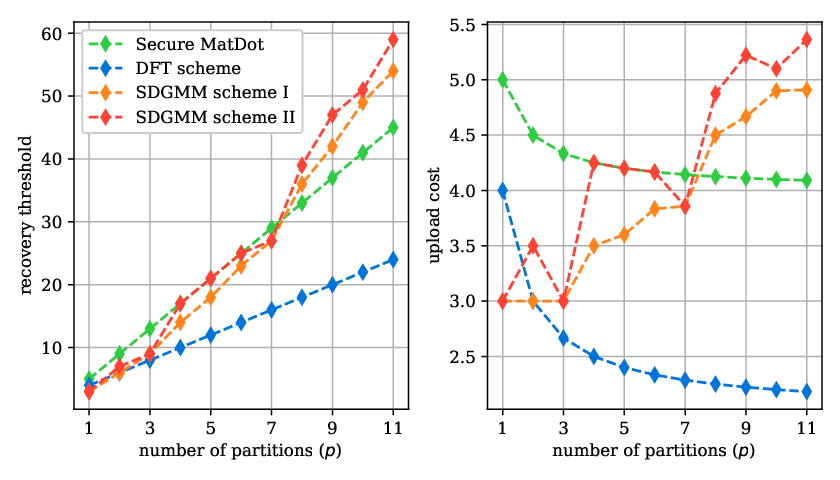
We wish to compare our proposed scheme to regular SDMM schemes in terms of the upload cost, due to the nature of our problem. It is natural to compare our scheme against the secure MatDot scheme, since it is able to achieve the lowest possible recovery threshold and upload cost according to the result in [14]. We will also compare our scheme to the DFT scheme in [4], which also uses the inner product partitioning. The GASP scheme is optimized to have a low download cost, while having a large upload cost, so we will not be comparing our proposed schemes to the GASP scheme. Gram matrix multiplication has also been studied in [10] with regard to linear regression using the Lagrange coded computation scheme. This scheme partitions the matrix similarly, but the workers need to compute significantly more compared to our proposed method. Hence, we will not be comparing our scheme to the one presented in [10], since it would be difficult to fix the amount of computation that is done.
Figure 1 shows the recovery threshold and upload cost as a function of . We compare our schemes to the other schemes by fixing the amount of computation performed at the workers. As Gram matrix multiplication takes about half as many multiplications, we can consider the secure MatDot and the DFT schemes with partitions and the SDGMM schemes with partitions. We see that our proposed schemes have a lower upload cost than the secure MatDot scheme for , which corresponds to workers. For larger values of we see that our proposed schemes are worse than the secure MatDot scheme. The DFT scheme has a lower upload cost, but it cannot tolerate stragglers like the other schemes.
The schemes proposed in this paper consider the case of , i.e., the case where the workers do not collude. It is straightforward to extend these schemes to colluding with workers, but it is not clear if the proposed schemes are optimal in this setting. We leave the case of for future work.
IV Analog Distributed Gram Matrix Multiplication
The proposed scheme in the previous section works over a finite field , but for practical applications in data science, it would be preferable to have a scheme that works over the analog domain, i.e., over or . The scheme can be adapted to work over the analog domain using similar methods that were done in [5] for regular SDMM schemes. These will give a tradeoff between the security and the numerical stability, but will achieve the same recovery thresholds and improvements over other schemes.
However, if security is not a concern, then the Gram matrix can be computed by the following analog distributed Gram matrix multiplication (ADGMM) scheme. Here is the conjugate transpose of . The matrix is partitioned to pieces horizontally. Define the polynomial
Let be distinct evaluation points such that for all . The worker receives and computes . These are evaluations of the function
since at the evaluation points , we have that . By multiplying this function with , we get a polynomial of degree , where the coefficient of is
This means that the Gram matrix can be recovered from any responses. This scheme matches the MatDot scheme, but the matrix is encoded only once, which means that the upload cost is reduced to half compared to the regular MatDot scheme. Additionally, the workers can utilize more efficient algorithms to compute the Gram matrices .
We can also study the degree table for this scheme, where we consider the differences of the degrees instead of the sums, since for our chosen evaluation points. For example, for , we get the following degree table.
| 0 | 1 | 2 | 3 | 4 | |
|---|---|---|---|---|---|
| 0 | 0 | -1 | -2 | -3 | -4 |
| 1 | 1 | 0 | -1 | -2 | -3 |
| 2 | 2 | 1 | 0 | -1 | -2 |
| 3 | 3 | 2 | 1 | 0 | -1 |
| 4 | 4 | 3 | 2 | 1 | 0 |
Adding security to this scheme is not obvious, since any noise term would contribute an interference term in the constant term, i.e., a zero on the diagonal by symmetry. In the secure MatDot scheme we are able to avoid this by not having a symmetric degree table.
Acknowledgements
This work has been supported by the Academy of Finland under Grant No. 336005 and by the Vilho, Yrjö and Kalle Väisälä Foundation of the Finnish Academy of Science and Letters.
References
- [1] W.-T. Chang and R. Tandon, “On the capacity of secure distributed matrix multiplication,” in 2018 IEEE Global Communications Conference (GLOBECOM). IEEE, 2018, pp. 1–6.
- [2] M. Aliasgari, O. Simeone, and J. Kliewer, “Distributed and private coded matrix computation with flexible communication load,” in 2019 IEEE International Symposium on Information Theory (ISIT). IEEE, 2019, pp. 1092–1096.
- [3] R. G. D’Oliveira, S. El Rouayheb, and D. Karpuk, “GASP codes for secure distributed matrix multiplication,” IEEE Transactions on Information Theory, vol. 66, no. 7, pp. 4038–4050, 2020.
- [4] N. Mital, C. Ling, and D. Gündüz, “Secure distributed matrix computation with discrete Fourier transform,” IEEE Transactions on Information Theory, 2022.
- [5] O. Makkonen and C. Hollanti, “Analog secure distributed matrix multiplication over complex numbers,” in 2022 IEEE International Symposium on Information Theory (ISIT), 2022, pp. 1211–1216.
- [6] M. Soleymani, H. Mahdavifar, and A. S. Avestimehr, “Privacy-preserving distributed learning in the analog domain,” arXiv preprint arXiv:2007.08803, 2020.
- [7] ——, “Analog Lagrange coded computing,” IEEE Journal on Selected Areas in Information Theory, vol. 2, no. 1, pp. 283–295, 2021.
- [8] Z. Jia and S. A. Jafar, “On the capacity of secure distributed batch matrix multiplication,” IEEE Transactions on Information Theory, vol. 67, no. 11, pp. 7420–7437, 2021.
- [9] J. Li and C. Hollanti, “Private and secure distributed matrix multiplication schemes for replicated or MDS-coded servers,” IEEE Transactions on Information Forensics and Security, vol. 17, pp. 659–669, 2022.
- [10] Q. Yu, S. Li, N. Raviv, S. M. M. Kalan, M. Soltanolkotabi, and S. A. Avestimehr, “Lagrange coded computing: Optimal design for resiliency, security, and privacy,” in The 22nd International Conference on Artificial Intelligence and Statistics. PMLR, 2019, pp. 1215–1225.
- [11] H. Yang and J. Lee, “Secure distributed computing with straggling servers using polynomial codes,” IEEE Transactions on Information Forensics and Security, vol. 14, no. 1, pp. 141–150, 2019.
- [12] J.-G. Dumas, C. Pernet, and A. Sedoglavic, “On fast multiplication of a matrix by its transpose,” in Proceedings of the 45th International Symposium on Symbolic and Algebraic Computation, 2020, pp. 162–169.
- [13] R. G. D’Oliveira, S. El Rouayheb, D. Heinlein, and D. Karpuk, “Degree tables for secure distributed matrix multiplication,” IEEE Journal on Selected Areas in Information Theory, vol. 2, no. 3, pp. 907–918, 2021.
- [14] O. Makkonen and C. Hollanti, “General framework for linear secure distributed matrix multiplication with byzantine servers,” in 2022 IEEE Information Theory Workshop (ITW). IEEE, 2022, pp. 143–148.