Hierarchy of Entanglement Renormalization and Long-Range Entangled States
Abstract
As a quantum-informative window into quantum many-body physics, the concept and application of entanglement renormalization group (ERG) have been playing a vital role in the study of novel quantum phases of matter, especially long-range entangled (LRE) states in topologically ordered systems. For instance, by recursively applying local unitaries as well as adding/removing qubits that form product states, the 2D toric code ground states, i.e., fixed point of topological order, are efficiently coarse-grained with respect to the system size. As a further improvement, the addition/removal of 2D toric codes into/from the ground states of the 3D X-cube model, is shown to be indispensable and remarkably leads to well-defined fixed points of a large class of fracton orders that are non-liquid-like. Here, we present a substantially unified ERG framework in which general degrees of freedom are allowed to be recursively added/removed. Specifically, we establish an exotic hierarchy of ERG and LRE states in Pauli stabilizer codes, where the 2D toric code and 3D X-cube models are naturally included. In the hierarchy, LRE states like 3D X-cube and 3D toric code ground states can be added/removed in ERG processes of more complex LRE states. In this way, a large group of Pauli stabilizer codes are categorized into a series of “state towers”; with each tower, in addition to local unitaries including (controlled-NOT) gates, lower LRE states of level- are added/removed in the level- ERG process of an upper LRE state of level-, connecting LRE states of different levels and unveiling complex relations among LRE states. As future directions, we expect this hierarchy can be applied to more general LRE states, leading to a unified ERG scenario of LRE states and exact tensor-network representations in the form of more generalized branching MERA (Multiscale Entanglement Renormalization Ansatz).
I Introduction
For the past decades, the goal of classification and characterization of novel quantum phases of matter has been indispensably intertwined with the surprisingly rapid progress on many-body quantum entanglement White 1992; White 1993; Schollwöck 2005; Vidal 2007; Aguado and Vidal 2008; Vidal 2008; König et al. 2009; Evenbly and Vidal 2014; Chen et al. 2010; Levin and Wen 2006; Li and Haldane 2008; Kitaev and Preskill 2006; Pollmann et al. 2010; Zeng et al. 2019; Gu and Wen 2009; Wen 2017. This line of efforts significantly reshapes modern many-body physics from the emphasis of entanglement structure instead of local correlation functions and local order parameters. For instance, the topologically ordered ground states of, e.g., fractional quantum Hall liquids Girvin 2005, chiral spin liquids Wen 1989, the toric code Kitaev 2006; Kitaev and Laumann 2009 and string-net models Levin and Wen 2005 have been identified as long-range entangled (LRE) states Chen et al. 2010 that cannot be adiabatically connected to (unentangled) product states by local unitary (LU) transformations, i.e., disentanglers. In contrast, short-range entangled states (SRE) can always be connected to product states by LU transformations. In particular, symmetry protected topological states (SPT) Chen et al. 2012, e.g., the Haldane spin chain, are a special class of SRE states in which all above-mentioned LU transformations inevitably break the global symmetry that protects SPT order. Remarkably, a series of stabilizer code models realizing topological orders are found to be fixed points of certain entanglement renormalization group (ERG) transformations Vidal 2007; Aguado and Vidal 2008; König et al. 2009 that simultaneously lead to an efficient representation of the topologically ordered ground state in terms of a tensor network, the multiscale entanglement renormalization ansatz (MERA) Vidal 2008; König et al. 2009; Evenbly and Vidal 2014. The idea of ERG provides a remarkable quantum-informative framework that significantly revolutionizes the traditional real-space and momentum-space renormalization-group treatments of quantum many-body systems and quantum field theory. More specifically, during the process of ERG transformations, LU transformations and addition/removal of product states are recursively performed, such that the number of qubits (i.e., the system size) and short-range entanglement can be coarse-grained while the long-range entanglement patterns (e.g., braiding and fusion data of 2D anyon systems) keep unaltered.
Recently, the concept of ERG transformations has been substantially advanced in order to unveil the quantum entanglement structure and fixed points of fracton orders—an exotic class of topologically ordered non-liquids Shirley et al. 2018; Haah 2014; Swingle and McGreevy 2016; Swingle and McGreevy 2016; Dua et al. 2020; Shirley et al. 2019; Wang et al. 2019; Shirley et al. 2022; Wen 2020; Wang 2022; Nandkishore and Hermele 2019; Pretko et al. 2020. In contrast to “pure” topological orders (e.g., the fractional quantum Hall states) that are liquid states, fracton orders are a kind of non-liquid-like LRE states whose local Hamiltonians support ground state degeneracy (GSD) that not only is locally indistinguishable (thus topologically ordered) but also grows subextensively with respect to the system size. For example, the GSD of X-cube model—the prototypical example of type-I fracton order—on a -torus satisfies that grows linearly with the linear system size Vijay et al. 2016. Immediately, it has been discovered that, to consistently define quantum phases and fixed points of fracton orders in the framework of entanglement renormalization, not only product states (i.e., SRE states), but also “pure” topological orders (i.e., a kind of LRE states) defined on lower dimensional space should be added/removed, such that two X-cube ground states of different system sizes can be adiabatically connected Shirley et al. 2018.

Despite the success of such ERG generalization, whether or not there is a much deeper mechanism towards a unified ERG framework is yet to be investigated.
In this paper, through exactly solvable models, we present a unified ERG framework via a hierarchical structure of ERG as well as the associated LRE states, where the above ERG transformations of original definition Vidal 2007; Aguado and Vidal 2008; König et al. 2009 and that of X-cube model Shirley et al. 2018 are naturally included. To be more specific, as shown in Fig. 1, we construct ERG transformations for a series of Pauli stabilizer code models Gottesman 1997 proposed in Ref. Li and Ye 2020, such that the models are fixed points of ERG transformations. All models we will study in this paper are uniquely denoted by four integers, i.e., , where a subset labeled by is found to be Pauli stabilizer code models with emergent gauge symmetry (see Sec. II for more details). The familiar 3D X-cube model is denoted as . And, we also successfully incorporate toric code models of all dimensions into the labeling system, which has not be included in Ref. Li and Ye 2020. For example, the 2D toric code model is labeled by . Remarkably, in the ERG transformations of these Pauli stabilizer codes, we find a hierarchical structure summarized in Fig. 1: in an ERG transformation connecting two states (i.e., the ground states of model as lattice Hamiltonian) with of different sizes, states are added/removed in addition to local unitaries (e.g., ), such that all Pauli stabilizer codes are fixed-points of the ERG transformations. While the of these topological non-liquid models grows polynomially with respect to the linear system size Li and Ye 2021, such ERG transformations are found to keep the GSD formulas consistent in different length scales. All in all, the ERG relation can be symbolically expressed as follows: where and are states of different sizes, and means the two sides can be connected by an LU transformation.
In the unified framework, ERG transformations obey the following rules:
-
In the ERG transformations on Pauli stabilizer codes considered here, LRE states are categorized into different levels, denoted as with the level index . Unentangled product states and more general SRE states are dubbed “level- LRE states” (denoted as symbolically) for the notational convenience;
-
ERG transformations where level- LRE states are added/removed are dubbed “level- ERG” (denoted as symbolically) transformations. Unless otherwise specified, is the highest level of added/removed LRE states;
-
States of the same stabilizer code with different sizes that can be connected by level- ERG transformations are identified as .
Then an transformation can be symbolically expressed as follows:
| (1) |
which explicitly shows a hierarchy of ERG transformations as well as LRE states along each upward arrow in Fig. 1. For example, the ERG of the 2D toric code is given by Vidal 2007; Aguado and Vidal 2008; König et al. 2009; Zeng et al. 2019:
| (2) |
where a toric code ground state is denoted as and product states denoted as are added/removed (note that SRE states are also symbolically denoted as for the notational convenience). Similarly, the ERG of the 3D X-cube model is given by Shirley et al. 2018:
| (3) |
where an X-cube ground state is denoted as and the 2D toric code ground state is added/removed.
We also note that, the above rules are established in the concrete stabilizer codes studied in this paper. In fact, Eq. (1) may be in principle a concrete realization of the following more general level- ERG transformation denoted as :
| (4) |
where is generally required. Assuming the existence of such transformations, a natural conjecture is that the level of LRE states may be decided by the transformations of the highest possible level. We leave such general ERG transformations as well as implied MERAs to further exploration.
The reminder of this paper is organized as follows. In Sec. II, we introduce some very useful geometric notations used in this paper and give a brief introduction to the models that include the 2D toric code model and the 3D X-cube model as special examples. Especially, we explain how to incorporate toric codes into the labeling system. Sec. III is dedicated to a detailed demonstration of some concrete ERG transformations. In Sec. III.1, as a warm-up, we perform the ERG transformations on the 2D toric code model (denoted as ), while an alternative approach was reviewed in Appendix C by following Ref. Zeng et al. 2019. In Sec. III.2, we review the ERG transformations on the 3D X-cube model (denoted as ). Then, we concretely construct the ERG transformations of different levels for and models respectively in Sec. III.3 and III.4. Sec. IV is dedicated to ERG transformations in general models. In Sec. IV.1, we demonstrate a general recipe for the ERG transformations of general models. In Sec. IV.2, we prove that the models are indeed fixed points of corresponding ERG transformations. Then, we demonstrate how these ERG transformations lead to the concept of a hierarchy of ERG transformations and LRE states in Sec. IV.3. A summary and outlook is given in Sec. V.
II Labeling system of Pauli stabilizer codes
This section is dedicated to the introduction of some background, including geometric notations and a family of Pauli stabilizer code models denoted by . Specially, we notice that models can be regarded as a -dimensional generalization of the 2D toric code model.
II.1 Geometric notations and lattice Hamiltonians
In this paper we need to involve some discussion about high dimensional geometric objects, so we believe it is beneficial to at first introduce some relevant notations. For a hypercubic lattice discussed in this paper, unless otherwise specified, we set lattice constant to be . Then, we introduce the concept of -cubes denoted by , that simply refers to -dimensional analogs of cube. For example, a (-cube) is simply a vertex, a (-cube) is a link, a (-cube) is a plaquette and a (-cube) is a conventional cube. In a -dimensional hypercubic lattice, with the above notations, we can use the coordinates of the center of a ( is assumed) to refer to the itself, as such a can be uniquely determined by the coordinates. Besides, we can see that the coordinate representation of a in a -dimensional hypercubic lattice is always composed of half-odd-integers (or hald-integer in shorthand) and integers. For example, in 3D cubic lattice, the coordinate representation of a (i.e. plaquette), such as and , always contains two half-integers and one integer. What’s more, following the terminology in Ref. Li and Ye 2020, we say a -cube and an -cube to be nearest to each other when for . Specially, when , we say they are nearest to each when . We can check that such a definition of being nearest is consistent with the usual conventions.
Next, we give a brief review of the definition of Pauli stabilizer code models. As lattice Hamiltonians, models is a subset of models proposed in Ref. Li and Ye 2020. In general, a model is defined on a -dimensional hypercubic lattice, with one -spin defined on each -cube (i.e. ). And the Hamiltonian is given as follows:
| (5) |
where a term is the product of the -components of the spins (a) being nearest to the -cube and (b) living in a -dimensional subsystem given by index , and an term is the product of the -components of the spins being nearest to the -cube . Here for simplicity, all coefficients of terms have been set to be . A concrete example of the Hamiltonian of (a.k.a. 3D X-cube) model is illustrated in Fig. 3(b). In Ref. Li and Ye 2020, is assumed, while in this paper, we allow the case to give a more complete picture of the hierarchy of ERG transformations and LRE states. More details of this case are given in Sec. II.2.
II.2 Incorporating toric codes
In this paper we primarily focus on models (i.e., we set , , ). Here, we notice that 2D and 3D toric code models can also be included into the above model series as and models respectively. In fact, generally a model can be recognized as a -dimensional generalization of 2D toric code model. Here, because models do not satisfy the condition, now the superscripts of terms are redundant, and a term is simply the product of the -components of the spins nearest to the .
To see the equivalence between a model and a -dimensional toric code model, we can consider a duality, where ’s are mapped to ’s, that can be concretely realized by shifting the coordinates of all ’s by . For a given model, upon the duality, we obtain a dual model that is still defined on a -dimensional hypercubic lattice, but -spins originally defined on ’s are now defined on ’s (a.k.a. links). As for the Hamiltonian terms, the original terms defined on ’s are mapped to terms defined on ’s (a.k.a. vertices), and the original terms defined on ’s are mapped to terms defined on ’s (a.k.a. plaquettes).
In summary, the Hamiltonian of the dual model defined on a -dimensional hypercubic lattice is given by , where each link is assigned with a -spin, is the product of -components of spins nearest to the vertex , is the product of -components of spins nearest to the plaquette (see Fig. 2 for the pictorial demonstration of some examples). Such a Hamiltonian is a -dimensional generalization of the 2D toric code model Hamma et al. 2005, and the ground states of which are regarded as states realized in different spatial dimensions (i.e., ). Note that the dual models themselves are not a part of models, thus in this paper the original models are more involved.

II.3 Ground state wavefunctions
Then, we can use a general recipe to obtain the ground states of stabilizer code models (including models, such as 2D and 3D toric codes). The lattice Hamiltonians of these models are all of the following form:
| (6) |
where and are some kinds of spatial locations (e.g. vertices, centers of links and centers of plaquettes) depending on the specific model, and the index in Eq. (5) has been formally absorbed into index for simplicity. Here, and are respectively local products of and Pauli operators, and they all commute with each other (see Fig. 3 for examples of and models). Therefore, a ground state of such a Hamiltonian has to satisfy constraints and (respectively denoted as and constraints). That is to say, for a given model, the and operators can be regarded as generators of a stabilizer group, and the ground state subspace is the corresponding stabilizer subspace Gottesman 1997; Zeng et al. 2019, as ground states are “stabilized” by all and operators. In this paper, as we mainly care about the stabilizer subspaces, unless otherwise specified, for a given model, we only consider states in its ground state subspace. Then, for an arbitrary stabilizer code model, we can obtain a ground state of it by the following procedures:
-
First, we consider basis, that is to say, we use Ising configurations, where spins are denoted by their direction along , as a basis of the whole Hilbert space. For a single qubit, we use the convention , (i.e., for spin up, and for spin down).
-
Second, we can notice that naturally satisfies all constraints. We denote as the reference state.
-
Third, we consider the equal weight superposition of the reference state and all configurations that can be obtained by applying a series of operators on the reference state, and denote this state as . As all and operators commute with each other, also satisfies constraints. According to our construction of , where configurations that can be related by the action of are always equally superpositioned, we can see that must also satisfy constraints. Hence, is a ground state of the stabilizer code model.
In the following part of this paper, we use an intuitive picture to describe an Ising configuration, by recognizing flipped spins (i.e. spin of the state ) as occupied by certain geometric objects. For example, if the spins are defined on links, then we recognize flipped spins as occupied by strings; and if the spins are defined on plaquettes, then we recognize flipped spins as occupied by membranes. For a model, other ground states can be obtained by applying logical operators on the state. Here in the basis, a logical operator can be recognized as a product of a series of operators, that commutes with all terms and do not equivalent to any product of a series of terms. For instance, in model defined on a (-torus), such a logical operator is a non-contractible closed string composed of operators Kitaev 2006; Kitaev and Laumann 2009.
Following this general recipe, we can see that when we ignore the topological degeneracy by focusing on the open boundary condition, we only need to consider the state, that can be regarded as a superposition of a series of configurations. For the state, terms require a superpositioned configuration to satisfy certain constraints, like flipped spins forming closed strings in model; terms require configurations that can be connected by action of terms to be equal-weight superpositioned. In Sec. III, a series of concrete examples are demonstrated in the corresponding subsections.

III Hierarchy of ERG transformations and LRE states
In this section, we concretely demonstrate the ERG transformations of some states. At first, in Sec. III.1 and Sec. III.2, we perform the ERG transformations of (2D toric code) and (3D X-cube) models respectively. Then, in Sec. III.3 and Sec. III.4, we respectively construct the ERG transformations of and models.
III.1 Level- ERG transformation of (2D toric code) states
The ERG transformations of states have been proposed and studied previously Aguado and Vidal 2008; König et al. 2009; Zeng et al. 2019, see the review in Appendix C. For consistency, here we perform an transformation of states in an explicitly different way. This alternative ERG process is very useful for designing ERG transformations of other models to be discussed in this paper.
At first, we give an intuitive picture of the states based on the general discussion in Sec. II. In (a.k.a. 2D toric code) model, spins are located at links of a 2D square lattice. In a superpositioned configuration of a state, a term requires vertex can only have , or flipped nearest spins, thus flipped spins must form closed strings. An term flips the spins on the links of plaquette , thus contractible closed strings can freely fluctuate in a ground state. We will see that, the ERG transformation indeed preserves this closed strings pattern of states.
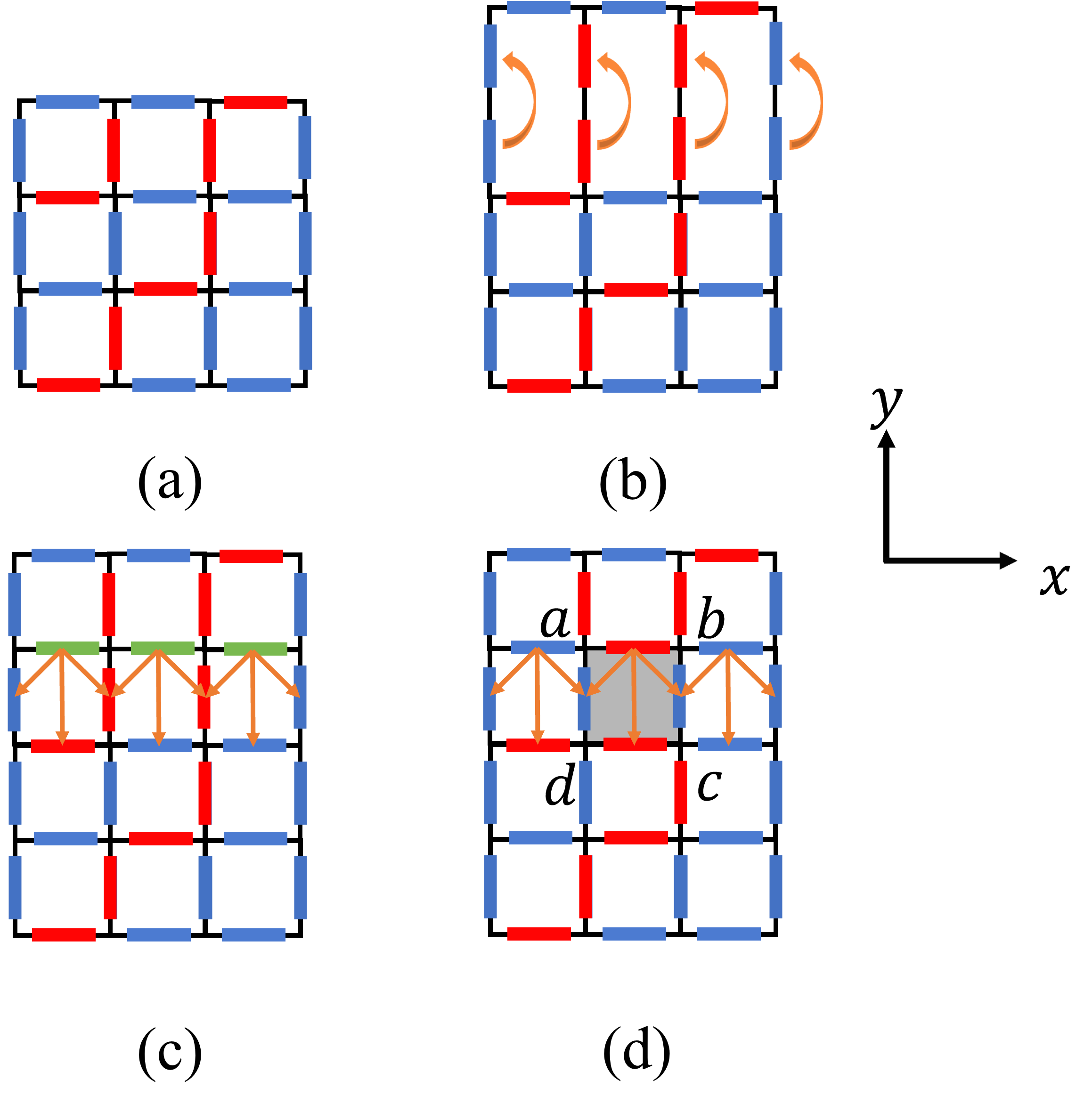
We start with a ground state of the model defined on a square lattice of the size with periodic boundary condition (PBC), and obtain a ground state on a square lattice of the size with PBC by the following transformations:
First, we choose a (-torus, a.k.a. loop) composed of the centers of parallel links along direction with the same -coordinate, and regard the as a cut: all links intersecting with the are cut into links. Without loss of generality, we assume the is located at , which means the cut links are of the form , where are integers. After that, we apply a rescaling. For each cut link , we double the length of to . Then, we can see that is cut into links and of length , and now the cut is located at . We assign the original spin on to .
Second, for each , we put an additional spin of the state on it. It means that we enlarge the Hilbert space by taking the tensor product of the original one and the added spins, and add a series of terms to the Hamiltonian to make all the added spins in the state (since a term requires a ground state to satisfy ). Then, for each original cut link , we apply a (controlled-NOT) gate with the original qubit on as control qubit and the added one on as target (see Fig. 4 (b)). By conjugate action of gates, the added terms are mapped to terms (see Appendix A). As a result, given a cut link , for an arbitrary Ising configuration from ( or ), we have , where . The ground state transformed by steps above is denoted as .
Third, we insert a product state of the size on the cut given in the first step, where is the eigenstate of with eigenvalue . That is to say, the spins composing the inserted state are located on links of the form in the rescaled lattice (see Fig. 4 (c), note that there are no spins on such links before this step). Then, we denote the tensor product of and as .
Finally, we act a series of gates on as illustrated in Fig. 4 (c) and (d). The gates are organized in a translational invariant manner, thus we only need to specify them for a specific plaquette. Without loss of generality, we take , and denote the vertices of by letters as shown in Fig. 4 (d). Concretely, we have and . Then, the gates can be explicitly specified as follows:
where refers to the spin located on the link between and vertices, points from the control qubit to target qubits.
We can straightforwardly check that after the application of the gates on , we obtain that preserves the closed strings pattern of states. To see this, we show that the by conjugate action, the gates generate all stabilizer generators we need to obtain states on the enlarged lattice. Firstly, by regarding as stabilized by a series of stabilizers with (i.e., for each stabilizer, the link where the stabilizer is defined satisfies ), under the conjugate action of gates, a stabilizer with is mapped to an term with ; then, a stabilizer obtained in the second step above is mapped to a term with ; finally, as we can notice that also in the second step above, an term with in the original lattice is mapped to a six-spin term composed of the components of all spins nearest to a rectangle (see Fig. 4 (b)), by taking the product of such a modified term and an term with , an arbitrary term with can be obtained. Therefore, the is indeed a state on the enlarged lattice. Or from another perspective, the model is a fixed point of the transformation, as symbolically expressed in Eq. (2).
III.2 Level- ERG transformation of (3D X-cube) states
In this subsection, we review the transformation of the states following the recipe in Ref. Shirley et al. 2018. Again, we firstly give an intuitive picture of the states based on the general discussion in Sec. II. In (a.k.a. 3D X-cube) model, spins are located at links of a 3D cubic lattice. In this case, terms with perpendicular , where denotes a plane containing vertex , require can only emanate perpendicular strings composed of flipped spins (see Fig. 5 (a)), thus flipped spins must form “cages” Prem et al. 2019 in a superpositioned configuration. An term flips the spins on the links of cube , thus contractible cages can freely fluctuate. We will see that, the ERG transformation indeed preserves this cage-net pattern of states.
We start with a ground state of the model defined on a cubic lattice of the size with PBC, and obtain a ground state on a cubic lattice of the size with PBC by the following transformations:
First, we choose a (-torus) composed of the centers of parallel links along direction with the same -coordinate, and regard the as a cut: all links intersecting with the are cut into links. Without loss of generality, we assume the is located at , which means the cut links are of the form , where are integers. After that, we apply a rescaling. For each cut link , we double the length of to . Then, we can see that is cut into links and of length , and now the cut is located at . We assign the original spin on to .
Second, for each , we put an additional spin of the state on it. It means that we enlarge the Hilbert space by taking the tensor product of the original one and the added spins, and add a series of terms to the Hamiltonian to make all the added spins in the state . Then, for each original cut link , we apply a gate with the original qubit on as control qubit and the added one on as target. By conjugate action of gates, the added terms are mapped to terms (see Appendix A). As a result, given a cut link , for an arbitrary Ising configuration from ( or ), we have , where (see Fig. 5 (b)). The ground state transformed by steps above is denoted as .
Third, we insert a (2D toric code) state of the size on the cut given in the first step. That is to say, the spins composing the inserted state are located on links of the form and in the rescaled lattice (see Fig. 5 (c), note that there are no spins on such links before this step). Then, we denote the tensor product of and as . As (2D toric code) model on a is -fold degenerated, this step has possible outcomes corresponding to possible inserted states.
Finally, we act a series of gates on as illustrated in Fig. 5 (d). The gates are organized in a translational invariant manner, thus we only need to specify them for a specific cube. Without loss of generality, we take , and denote the vertices of by letters as shown in Fig. 5 (d). For example, we have and . Then, the gates can be explicitly specified as follows:
where refers to the spin located on the link between and vertices, points from the control qubit to target qubits. Intuitively, we can see that by conjugate action (see Apppendix A), the gates map the stabilizer of the inserted state to , that is a stabilizer of (3D X-cube) state. Similarly, we can check that the gates generate all stabilizer generators we need to obtain states on a lattice of the size with PBC (see Sec. IV.2 for a more detailed demonstration).
Therefore, after the application of the gates on , we obtain , which is a ground state of (3D X-cube) model on a lattice of the size with PBC. Pictorially, we can see the transformed state preserves the cage-net pattern of states.
Due to the fact that there are possible choices of in the third step, for a given , we have possible outcomes. As a result, if we require the GSD formula to be symmetric for , and , the GSD of model has to satisfy , where is a constant. This result is consistent with the exact result given in Ref. Vijay et al. 2016; Li and Ye 2021. Besides, based on this method to obtain the GSD, it has been shown in Ref. Shirley et al. 2018 that the coefficients of linear terms in the are directly related to the topology of the 2D subsystems (dubbed as “leaves”) of model.

III.3 Level- ERG transformation of states
In this subsection, we demonstrate the transformation of states. Similar to model, here we give an intuitive picture of states based on the general discussion in Sec. II. In model, spins are located at links of a 4D hypercubic lattice. In this case, terms with perpendicular , where denotes a plane containing vertex , require can only emanate perpendicular strings composed of flipped spins. An term flips the spins on the links of hypercube . We will see that, the ERG transformation indeed preserves the pattern of states.
Again, we start with a ground state of the model defined on a lattice of the size with PBC, and obtain a ground state on a lattice of the size with PBC. The transformation can be described as follows:
First, we choose a (-torus) composed of the centers of parallel links along direction with the same -coordinate, and regard the as a cut: all links intersecting with the are cut into links. Without loss of generality, we assume the is located at , which means the cut links are of the form , where are integers. After that, we apply a rescaling. For each cut link , we double the length of to . Then, we can see that is cut into links and of length , and now the cut is located at . We assign the original spin on to .
Second, for each , we put an additional spin of the state on it. It means that we enlarge the Hilbert space by taking the tensor product of the original one and the added spins, and add a series of terms to the Hamiltonian to make all the added spins in the state . Then, for each original cut link , we apply a gate with the original qubit on as control qubit and the added one on as target. By conjugate action of gates, the added terms are mapped to terms (see Appendix A). As a result, given a cut link , for an arbitrary Ising configuration from ( or ), we have , where . The ground state transformed by the steps above is denoted as .
Third, we insert a (3D X-cube) state of the size on the cut given in the first step. That is to say, the spins composing the inserted state are located on links of the form , and in the rescaled lattice (note that there are no spins on such links before this step). Then, we denote the tensor product of and as . As (3D X-cube) model on the satisfies , this step has possible outcomes corresponding to possible inserted states.
Finally, we act a series of gates on as illustrated in Fig. 6. The gates are organized in a translational invariant manner, thus we only need to specify them for a specific -cube. Without loss of generality, we take , and denote the vertices of by letters as shown in Fig. 6. Then, the gates can be explicitly specified as follows:
where refers to the spin located on the link between and vertices, points from the control qubit to target qubits. Intuitively, we can see that by conjugate action (see Apppendix A), the gates map the
stabilizer of the inserted state to
that is a stabilizer of ground state. Similarly, we can check that the gates generate all stabilizer generators we need to obtain ground states on a lattice of the size with PBC (see Sec. IV.2 for a more detailed demonstration). Therefore, after the application of the gates on , we obtain , which is a ground state of model on a lattice of the size with PBC.
Similar to model, we can see that the GSD of model has to satisfy , where is a function of , and . When we require the GSD formula to be symmetric for , , and , then we have , where is a constant. This result is consistent with the result obtained by ground state decomposition in Ref. Li and Ye 2021.

III.4 Level- ERG transformation of states
For comparison, in this subsection, we demonstrate the transformation of states. We will see that, though model has the same spatial dimension as model, in the ERG transformation of its ground states we only need to add/remove rather than states. Before the demonstration, here we also give an intuitive picture of states based on the general discussion in Sec. II. In model, spins are located at plaquettes of a 4D hypercubic lattice. In this case, terms with perpendicular , where denotes a 3D subsystem containing link , require can only emanate perpendicular membranes composed of flipped spins. An term flips the spins on the plaquettes of hypercube . We will see that, the ERG transformation indeed preserves the pattern of states.
Again, we start with a ground state of the model defined on a lattice of the size with PBC, and obtain such a ground state on a lattice of the size with PBC. The transformation can be similarly described as follows:
First, we choose a (-torus) composed of the centers of parallel links along direction with the same -coordinate, and regard the as a cut: all plaquettes intersecting with the are cut into plaquettes. Without loss of generality, we assume the is located at , which means the cut plaquettes are of the form , where , is the unit vector along direction, are integers. After that, we apply a rescaling. For each cut plaquette , we double the linear size of along direction to . Then, we can see that is cut into plaquettes and with linear sizes along direction equal to , and now the cut is located at . We can assign the original spin on to .
Second, for each , we put an additional spin of the state on it. Equivalently, it means that we enlarge the Hilbert space by taking the tensor product of the original one and the added spins, and add a series of terms to the Hamiltonian to make all the added spins in the state . Then, for each original cut plaquette , we apply a gate with the original qubit on as control qubit and the added one on as target. By conjugate action of gates, the added terms are mapped to terms (see Appendix A). As a result, given a cut plaquette , for an arbitrary Ising configuration from ( or ), we have , where . The ground state transformed by the steps above is denoted as .
Third, we insert a (3D toric code) state of the size on the cut given in the first step. That is to say, the spins composing the inserted state are located on plaquettes of the form , and in the rescaled lattice (note that there are no spins on such plaquettes before this step). Then, we denote the tensor product of and as . As (3D toric code) model on the satisfies Hamma et al. 2005; Kong et al. 2020, this step has possible outcomes corresponding to possible inserted states.
Finally, we act a series of gates on as illustrated in Fig. 7. The gates are organized in a translational invariant manner, thus we only need to specify them for a specific -cube. Without loss of generality, we take , and denote the vertices of by letters as shown in Fig. 7. Then, the gates can be explicitly specified as follows:
where refers to the spin located on the plaquette between , , and vertices, points from the control qubit to target qubits. Intuitively, we can see that by conjugate action (see Apppendix A), the gates map the
stabilizer of the inserted state to
that is a stabilizer of ground state. Similarly, we can check that the gates generate all stabilizer generators we need to obtain ground states on a lattice of the size with PBC (see Sec. IV.2 for a more detailed demonstration). Therefore, after the application of the gates on , we obtain , which is a ground state of model on a lattice of the size with PBC.
Similar to model, we can see that the GSD of model has to satisfy , where is a function of and . When we require the GSD formula to be symmetric for , , and , then we have , where is a constant. This result is consistent with the result obtained by ground state decomposition in Ref. Li and Ye 2021.

IV ERG of generic levels
In this section, we firstly show a generic recipe of the construction of transformations of models with . After that, in Sec. IV.2, we prove that for such a model, the constructed ERG transformation indeed gives ground states of the same model of different sizes, i.e., the models are fixed points of the corresponding ERG transformations. Finally, in Sec. IV.3, we discuss about the hierarchy of ERG transformations and LRE states based on the constructed ERG transformations. Note that transformations of models are not included in this recipe.
IV.1 Level- ERG transformation of states
In general, for a model with , we can demonstrate the transformation of states. Again, we start with a ground state of model defined on a lattice of the size with PBC, and obtain a ground state on a lattice of the size with PBC. The transformation can be described as follows:
-
First, we choose a -torus composed of the centers of links with the same -coordinate. Without loss of generality, we set the chosen to be located at , such that it is composed of the centers of links of the form , where are integers. Then we regard the as a cut: every intersecting with the is cut into ’s with identical spins. That is to say, for each cut , we put an additional spin in the state , and then apply a gate with the original qubit as control qubit and the added one as target. In consequence, given a cut , for an arbitrary Ising configuration from ( or ), we have , where . Then, we rescale the lattice by extending the linear size of the cut along direction to , such that now the chosen is composed of sites of the form , and for a cut in the original lattice, the original and additional spins are respectively assigned to and in the rescaled lattice. The ground state transformed by this step is denoted as .
-
Second, we put a ground state of the size on the given in the previous step. That is to say, we can regard the sites as forming a hypercubic lattice defined on the , and consider a ground state defined on this lattice. Then, by taking the tensor product of and , we obtain .
-
Third, we act an LU transformation composed of a series of gates on (see Sec. IV.2 for a demonstration of this LU transformation ). After that, we obtain , which is a ground state of model on a lattice of the size with PBC.
To see that this generic recipe is consistent with the GSD results obtained by ground state decomposition in Ref. Li and Ye 2021, without loss of generality, say that in the polynomial of model on the , the coefficient of term is (here is assumed). Then, the above ERG transformation requires that the number of copies of contained in the of model grows linearly with . That is to say, the polynomial of the model has to contain the term . This result is consistent with the relevant results from Ref. Li and Ye 2021.
IV.2 models as fixed points of level- ERG transformations
In this subsection, we give the conditions that an LU transformation used in the Step 3 of the transformation of a general state should satisfy, and prove that the such an LU transformation indeed gives ground states of the model on a lattice of different sizes, by considering the conjugate action of on the Hamiltonian terms. Without loss of generality, we assume the cut is extended along , , directions, and the location is given by (in the rescaled lattice). For convenience, here we explicitly write down the Hamiltonian of a model as below:
| (7) |
where an term is the product of the -components of the spins nearest to the , a term is the product of the -components of the spins that are (a) nearest to the and (b) living in the -dimensional subsystem .
We start with the conditions that the LU transformation should satisfy. According to the LU transformation of , and models (i.e., the gates applied on states of corresponding subsections), we expect such an LU transformation in the transformation of a general state to satisfy the following conditions:
-
First, we require to be composed of a series of gates around ’s with , where all control qubits are from the cut (i.e., being located on ’s with ). Besides, we require to be translational invariant, such that the application of the gates is the same for every applied . Therefore, we only need to consider the application of gates in a single to specify . Without loss of generality, we can focus on . Here the superscript is for reference.
-
Second, for each in with , we require the qubit on it to be controlled by the qubit on , where is the unit vector along direction. Obviously, the qubit on such a is only controlled by control qubit in .
-
Third, for each in with , we require the qubit on it to be controlled by exactly nearest control qubit in . Besides, for a pair of nearest parallel qubits, we require them to be simultaneously controlled (or not) by the control qubit that links them. For example, a pair of nearest parallel qubits respectively defined on and are either both controlled by or not (here we can notice that this control qubit is the only one that links the pair, i.e., simultaneously being nearest to the pair of qubits).
The existence of such LU transformations is obvious. And we can check that when (a) , (b) and (c) , the LU transformations in the ERG transformations of , and states all satisfy the above conditions. Besides, here we should notice that each target qubit with is always controlled by two qubits. Without loss of generality, say the qubit on -cube is controlled by the qubit on , according to the translational invariance of the LU transformation, the qubit on must be controlled by the qubit on ; after that, as and are parallel -cubes connected by , must also be controlled by the qubit on . Then, we can notice that an arbitrary nearest to has the form , thus it must be either nearest to or . Since a target qubit can only be controlled by control qubit from a nearest as required by the conditions above, no other qubits in the can control . In conclusion, for any target qubit with , there are always qubits that control it.
Then, we show that though the concrete form of the LU transformation has not been specified, the above conditions can make sure that produces the ground states as expected. That is to say, for an LU transformation satisfying the conditions above, a is indeed a ground state of model.
At first, we notice that is applied on the given in Sec. IV.1, and can be obtained as a ground state of the following Hamiltonian:
| (8) |
where refers to the terms in the original model with some modifications according to the cut ’s (see below), refers to the terms of the Hamiltonian on the cut , and is added to make each pair of spins on a cut identical, where refers to a -cube with in the rescaled lattice. Note that the terms in near the are modified to to be consistent with the cut ’s, where and have the same form as an ordinary term from the original model, and satisfies . As a concrete example, in model, where , , such a modified , denoted as , is given by , where operators and themselves do not present in . Furthermore, for a term from with that involves qubit with , we can replace it by the product of the term itself and a corresponding term, such that the in the term is replaced by . This modification makes such terms “connected”. For example, in model, due to our assignment that for a cut link the original qubit is put on a link of the form , in the rescaled lattice, we would have terms such as , that is not connected, without such modifications. Similarly, we can freely add terms with to as such terms can be directly obtained by taking the products of terms with and corresponding terms. Besides, contains no terms on the . After that, we can see that all terms in still commute with each other. From another perspective, can also be be obtained by considering the conjugate action of the gates applied in the first step in Sec. IV.1. A more detailed demonstration of the terms in is given in Appendix B.
Secondly, because the transformation is a product of a series of gates, the conjugate action of on an arbitrary stabilizer can be reduced to the conjugate action of gates on . With the general mapping rules given by the conjugate action of gates (see Appendix A), we can obtain all terms in as follows:
-
First, since for an arbitrary inside the , all qubits that are controlled by the qubits from the together with the control qubits themselves form a with , terms in are mapped to terms with .
-
Second, since an arbitrary target qubit with is controlled by exactly qubits from the , each term in is mapped to a -spin term composed of the original , and the components of the qubits that control .
-
Third, further considering that an arbitrary target qubit with is only controlled by from the , a term in near the should be modified as follows: (a) for a qubit with involved in the term, multiply the term by ; (b) for a qubit with involved in the term, multiply the term by the components of the qubits that control the . As an example, for a term only involving qubits with , it is mapped to a term, where is obtained by adding to the coordinates of all qubits involved in .
-
Finally, all other terms stay invariant under the conjugate action of .
We denote the Hamiltonian of model on the lattice of the size with PBC as (see Eq. (7)). Then we can notice that by taking the product of terms obtained in the first step and terms from we can obtain all terms that exist in but superficially missing in ; by taking the product of the -spin terms obtained in the second step (which can be recognized as terms in ), modified terms obtained in the third step and terms in we can obtain all terms that exist in but superficially missing in . Therefore, all terms of can be obtained by taking the product of terms of (a more detailed demonstration is given in Appendix B). As it is also straightforward to check the other way around, finally, we can see that and are equivalent Pauli stabilizer code models with equivalent stabilizer groups, and is indeed a ground state of .
IV.3 Discussions
As we have demonstrated in this section, in the ERG transformations of different states, the added/removed states are also different LRE states. From another word, the entanglement patterns in states with different and a fixed are intrinsically different, and these models cannot be fully understood as fixed points of a finite number of types of ERG transformations. Instead, we need an infinite series of ERG transformations of different levels to understand the more general long range entanglement patterns.
Therefore, we conclude the above observations by proposing the concept of a hierarchy of ERG transformations, where each transformation is assigned with an integer level. Correspondingly, LRE states are assigned with integer levels as well (see Fig. 1). For a given stabilizer code model considered in this paper, two level- LRE () states of different sizes can be connected by a level- ERG () transformation, that is composed of LU transformations combined with addition/removal of level- LRE states. Furthermore, if we define product states and short range entangled states as states, then we have (2D toric code) states as states, (3D X-cube) states as states, states as states and so on. Besides, we can see that low level LRE states themselves can be recognized as trivial high level LRE states, just like a product state is recognized as a trivial “pure” topological order. Specially, a decoupled stack of states is also a trivial state, as it can reduced to nothing under a transformation.
V Summary and outlook
In this paper, by considering a class of Pauli stabilizer codes, we constructed a more unified ERG framework through adding/removing more general degrees of freedom. The well-established ERG processes of the (2D toric code) and (3D X-cube) model are naturally included as the simplest cases. All Pauli stabilizer codes considered here are categorized into a series of “state towers” as shown in Fig. 1; in each tower, lower LRE states of level- are added/removed in the level- ERG process of an upper LRE state of level-. Several future directions are listed below.
First, we may expect a more general ERG framework shown in Eq. (4) can be constructed in other stabilizer codes.
Second, the completeness of the concept of level of LRE states needs further exploration. For example, for type-II fracton ordered states Haah 2011; Vijay et al. 2016; Vijay et al. 2015, such as Haah’s code Haah 2011, a series of ERG transformations have been constructed and studied Dua et al. 2020; Haah 2014; Swingle and McGreevy 2016, nevertheless, whether it is possible to consistently assign a level to such Type-II fracton ordered states and corresponding ERG transformations is yet to be determined. Some further discussion about the hierarchy of ERG transformations may be beneficial for a more complete understanding of the entanglement patterns in more generic fracton orders.
Third, except for the stabilizer code models considered in this paper, physically, we can also consider models perturbed by external fields, which are no longer exactly solvable. Constructing ERG transformations for such models to investigate their fixed points is also an interesting direction. And some numerical techniques may also be useful in the study of such models Mühlhauser et al. 2020; Zhou et al. 2022; Zhu et al. 2022.
Finally, it is known that the ERG transformations are related to MERA, that is a kind of tensor networks capable of efficiently encoding the entanglement signatures of certain quantum many-body states Vidal 2008; König et al. 2009; Evenbly and Vidal 2014; Evenbly and Vidal 2014. In Ref. Shirley et al. 2018, it has been noticed that (3D X-cube) states bear exact branching MERA representations. Then it is natural to ask whether LRE states of general levels can have such tensor network representations. If so, the holographic geometries generated by such tensor networks are also worth exploring Evenbly and Vidal 2011; Swingle 2012; Evenbly 2017.
Acknowledgements.
This work was supported by NSFC Grant No. 12074438, Guangdong Basic and Applied Basic Research Foundation under Grant No. 2020B1515120100, the Fundamental Research Funds for Central Universities (22qntd3005), and the Open Project of Guangdong Provincial Key Laboratory of Magnetoelectric Physics and Devices under Grant No. 2022B1212010008.Appendix A A brief introduction of controlled-NOT () gate
Here we give a brief introduction of the controlled-NOT () gate that is to be frequently used in the main text of this paper.
By definition, gate is a 2-qubit unitary operation. In basis, for , where , gate maps to , here means tensor product, means modulo addition. Effectively, gate regards the first qubit as a control qubit, and the second qubit as a target qubit. When the control (first) qubit is , then gate does nothing; when the control qubit is , gate flips the target (second) qubit, thus the name. For example, denoting the action of gate as , we have and .
For the usage in the main text, here we also introduce the conjugate action of gate on stabilizers (i.e., Hamiltonian terms of a stabilizer code model and their products). For a state in the stabilizer subspace and a stabilizer (i.e. ), if we apply a gate on , then we have . That is to say, the transformed state is stabilized by , that is acted by the conjugate action of the gate. For a specific acting non-trivially on some control or target qubits, the correspondence between and can be expressed as followsShirley et al. 2018; Aguado and Vidal 2008:
where the first qubit refers to the control qubit, and the second qubit refers to the target qubit. For example, if we consider the conjugate action of a gate on a stabilizer , where applies a on the control qubit, and applies an identity on the target qubit, then the corresponding will apply on both qubits.
Appendix B Proof of the equivalence between Hamiltonians and
In this appendix, we concretely demonstrate that in Sec. IV.2, all terms in , the Hamiltonian of model on the lattice of the size with PBC, can be obtained by taking the product of terms in and vice versa, thus they are equivalent stabilizer code models. As we can notice that and only have different terms around the with , we only need to consider terms defined on locations with .
Before discussing about terms in , we would to like to give a detailed demonstration and classification of the terms around the cut in . Such terms in can be classified as follows:
- •
terms: terms with from that only involve qubits with .
- •
terms: terms with from that simultaneously involve qubits with and .
- •
terms: terms with from .
- •
terms: terms with from (i.e. such terms only involve qubits with ).
- •
terms: terms with from .
- •
terms: terms with from .
- •
terms: terms with from .
- •
terms: with from .
And we can notice that, around the , is composed of , , , , , and the following terms:
- •
terms: terms with that involve qubits with .
- •
terms: terms with .
Then, we consider the conjugate action of the LU transformation on the terms in , that leads to terms in (note that here the superscripts of terms are omitted as we only need to consider the types of terms):
- •
A term is mapped to , the product of the term itself and a term .
- •
A term is mapped to (a) the term itself, if the qubits with and in are controlled by the same pair of qubits from the ; (b) , the product of the term itself and a term , if otherwise.
- •
A term is mapped to (a) the term itself, if perpendicular qubits in (i.e., the qubits are nearest and from different -dimensional subsystems) share control qubit; (b) , the product of the term itself and terms and , if perpendicular qubits in have control qubits that nearest to the same ; (c) , the product of the term itself and terms , , and , if otherwise;
- •
, , terms stay invariant.
- •
An term terms with is mapped to an term with , where the is obtained by .
- •
A term term is mapped to a term with , where the is obtained as .
Because , , terms are invariant under the conjugate action of (i.e., they present in ), we can obtain an arbitrary , or term by taking the product of the corresponding transformed term with invariant terms. An arbitrary term with can be obtained as a transformed term, and an arbitrary term with can be obtained by taking the product of a transformed term and an invariant term. Besides, by taking the product of a transformed term with a term, an arbitrary term can also be obtained. Finally, because it is straightforward to check that all terms in can be obtained by taking products of terms in , as two stabilizer code models, and have equivalent sets of stabilizer generators, thus the stabilizer subspaces should be equivalent.
Appendix C Another level- ERG transformation of states
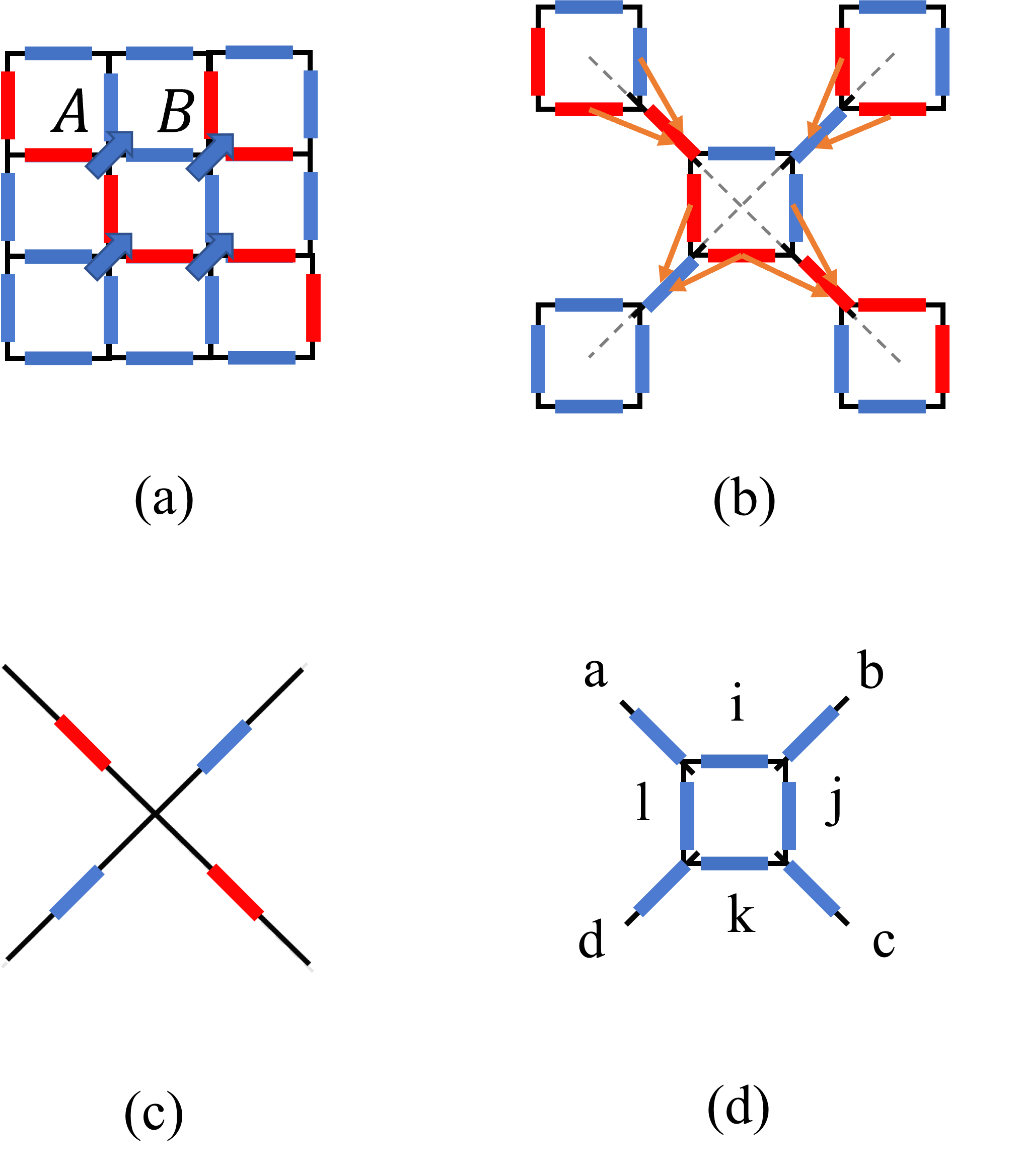
In this appendix, we review the transformation of (2D toric code) states following the recipe in Ref. Zeng et al. 2019. In this transformation of a state defined on a square lattice with PBC, we firstly separate vertices into A and B sublattices. Then, we put an additional -spin in state on each vertex (see Fig. 8(a)). After that, we apply an LU transformation , that is composed of a series of gates: for each additional spin, we act two gates targeting on it. More specifically, for an additional qubit in sublattice A, we use the qubits on the up and left links as control qubits; for an additional qubit in sublattice B, we use qubits on the up and right links (see Fig. 8(b)). The action of can be understood pictorially: recall that in any allowed Ising configuration of a state there must be either an even number or zero of spins around each vertex, thus flipped spins always form closed strings. Then, we can notice that the design of gates in exactly preserves this constraint by integrating additional spins into the closed strings pattern.
After that, we further apply an LU transformation to map the spins around each square to (normalization is omitted), and such spins can be removed out of the state as can be transformed to a product state by a local unitary operator. For the lattice, the LU transformation and the removal of spins effectively shrinks every square to a vertex as shown in Fig. 8(c). By noticing that in each configuration there is always an even number or zero of diagonal links around each square with qubits in , the resulting state also has the closed strings pattern. Here, to see that is indeed an LU transformation, we can recognize , which is the product of operators supported around each square . A acts on the four qubits on links nearest to the square (denoted by , , and ) and the four qubits on the diagonal links around (denoted by , , and , see Fig. 8(d)). Here, can be roughly recognized as a generalized gate: it takes the qubits on diagonal links as control qubits, and qubits on the square as targets. For a specific configuration of the eight qubits, the action of can be obtained as follows: a) if all control qubits are , then flip no target qubits; b) if two control qubits are , then flip the target qubits between them clockwise following the alphabetical order (e.g. if qubits on and are , then flip qubits on and ); c) if all control qubits are in , then flip qubits on and . Then, obviously satisfies , thus . Next, notice that Ising configurations form a complete basis of the Hilbert space, for an arbitrary pair of Ising configurations of the eight qubits and , we can obtain that : we only have when the control qubits in and are all the same, and only the qubits to be flipped are different in and ; otherwise, . As a result, , thus is both unitary and Hermitian. Since the transformations above do not change the pattern that the state is invariant under the action of terms on squares, and always maps the configuration of a square to or , we can see that spins nearest to each square are indeed mapped to .
Finally, we obtain a state on a square lattice with a larger lattice constant. That is to say, after an ERG transformation composed of adding/removing product states and LU transformations, the structure of the state is preserved. Or from another perspective, the model is a fixed point of the transformation as symbolically expressed in Eq. (2). A pictorial demonstration of this ERG transformation is given in Fig. 8.
References
- White (1992) Steven R. White, “Density matrix formulation for quantum renormalization groups,” Phys. Rev. Lett. 69, 2863–2866 (1992).
- White (1993) Steven R. White, “Density-matrix algorithms for quantum renormalization groups,” Phys. Rev. B 48, 10345–10356 (1993).
- Schollwöck (2005) U. Schollwöck, “The density-matrix renormalization group,” Rev. Mod. Phys. 77, 259–315 (2005).
- Vidal (2007) G. Vidal, “Entanglement renormalization,” Phys. Rev. Lett. 99, 220405 (2007).
- Aguado and Vidal (2008) Miguel Aguado and Guifré Vidal, “Entanglement Renormalization and Topological Order,” Phys. Rev. Lett. 100, 070404 (2008), arXiv:0712.0348 [cond-mat.str-el] .
- Vidal (2008) G. Vidal, “Class of quantum many-body states that can be efficiently simulated,” Phys. Rev. Lett. 101, 110501 (2008).
- König et al. (2009) Robert König, Ben W. Reichardt, and Guifré Vidal, “Exact entanglement renormalization for string-net models,” Phys. Rev. B 79, 195123 (2009), arXiv:0806.4583 [cond-mat.str-el] .
- Evenbly and Vidal (2014) G. Evenbly and G. Vidal, “Class of Highly Entangled Many-Body States that can be Efficiently Simulated,” Phys. Rev. Lett. 112, 240502 (2014), arXiv:1210.1895 [quant-ph] .
- Chen et al. (2010) Xie Chen, Zheng-Cheng Gu, and Xiao-Gang Wen, “Local unitary transformation, long-range quantum entanglement, wave function renormalization, and topological order,” Phys. Rev. B 82, 155138 (2010).
- Levin and Wen (2006) Michael Levin and Xiao-Gang Wen, “Detecting Topological Order in a Ground State Wave Function,” Phys. Rev. Lett. 96, 110405 (2006), arXiv:cond-mat/0510613 [cond-mat.str-el] .
- Li and Haldane (2008) Hui Li and F. D. M. Haldane, “Entanglement Spectrum as a Generalization of Entanglement Entropy: Identification of Topological Order in Non-Abelian Fractional Quantum Hall Effect States,” Phys. Rev. Lett. 101, 010504 (2008).
- Kitaev and Preskill (2006) Alexei Kitaev and John Preskill, “Topological Entanglement Entropy,” Phys. Rev. Lett. 96, 110404 (2006), arXiv:hep-th/0510092 [hep-th] .
- Pollmann et al. (2010) Frank Pollmann, Ari M. Turner, Erez Berg, and Masaki Oshikawa, “Entanglement spectrum of a topological phase in one dimension,” Phys. Rev. B 81, 064439 (2010).
- Zeng et al. (2019) Bei Zeng, Xie Chen, Duan-Lu Zhou, Xiao-Gang Wen, et al., Quantum information meets quantum matter (Springer, 2019).
- Gu and Wen (2009) Zheng-Cheng Gu and Xiao-Gang Wen, “Tensor-entanglement-filtering renormalization approach and symmetry-protected topological order,” Phys. Rev. B 80, 155131 (2009).
- Wen (2017) Xiao-Gang Wen, “Colloquium: Zoo of quantum-topological phases of matter,” Rev. Mod. Phys. 89, 041004 (2017).
- Girvin (2005) Steven M Girvin, “Introduction to the fractional quantum hall effect,” in The quantum Hall effect (Springer, 2005) pp. 133–162.
- Wen (1989) X. G. Wen, “Vacuum degeneracy of chiral spin states in compactified space,” Phys. Rev. B 40, 7387–7390 (1989).
- Kitaev (2006) Alexei Kitaev, “Anyons in an exactly solved model and beyond,” Ann. Phys. 321, 2–111 (2006).
- Kitaev and Laumann (2009) Alexei Kitaev and Chris Laumann, “Topological phases and quantum computation,” Les Houches Summer School “Exact methods in low-dimensional physics and quantum computing 89, 101 (2009).
- Levin and Wen (2005) Michael A. Levin and Xiao-Gang Wen, “String-net condensation: A physical mechanism for topological phases,” Phys. Rev. B 71, 045110 (2005).
- Chen et al. (2012) Xie Chen, Zheng-Cheng Gu, Zheng-Xin Liu, and Xiao-Gang Wen, “Symmetry-protected topological orders in interacting bosonic systems,” Science 338, 1604–1606 (2012).
- Shirley et al. (2018) Wilbur Shirley, Kevin Slagle, Zhenghan Wang, and Xie Chen, “Fracton models on general three-dimensional manifolds,” Phys. Rev. X 8, 031051 (2018).
- Haah (2014) Jeongwan Haah, “Bifurcation in entanglement renormalization group flow of a gapped spin model,” Phys. Rev. B 89, 075119 (2014), arXiv:1310.4507 [cond-mat.str-el] .
- Swingle and McGreevy (2016) Brian Swingle and John McGreevy, “Renormalization group constructions of topological quantum liquids and beyond,” Phys. Rev. B 93, 045127 (2016).
- Swingle and McGreevy (2016) Brian Swingle and John McGreevy, “Mixed s -sourcery: Building many-body states using bubbles of nothing,” Phys. Rev. B 94, 155125 (2016), arXiv:1607.05753 [cond-mat.str-el] .
- Dua et al. (2020) Arpit Dua, Pratyush Sarkar, Dominic J. Williamson, and Meng Cheng, “Bifurcating entanglement-renormalization group flows of fracton stabilizer models,” Phys. Rev. Research 2, 033021 (2020).
- Shirley et al. (2019) Wilbur Shirley, Kevin Slagle, and Xie Chen, “Foliated fracton order in the checkerboard model,” Phys. Rev. B 99, 115123 (2019), arXiv:1806.08633 [cond-mat.str-el] .
- Wang et al. (2019) Taige Wang, Wilbur Shirley, and Xie Chen, “Foliated fracton order in the Majorana checkerboard model,” Phys. Rev. B 100, 085127 (2019), arXiv:1904.01111 [cond-mat.str-el] .
- Shirley et al. (2022) Wilbur Shirley, Xu Liu, and Arpit Dua, “Emergent fermionic gauge theory and foliated fracton order in the Chamon model,” arXiv e-prints , arXiv:2206.12791 (2022), arXiv:2206.12791 [cond-mat.str-el] .
- Wen (2020) Xiao-Gang Wen, “Systematic construction of gapped nonliquid states,” Phys. Rev. Research 2, 033300 (2020).
- Wang (2022) Juven Wang, “Nonliquid cellular states: Gluing gauge-higher-symmetry-breaking versus gauge-higher-symmetry-extension interfacial defects,” Phys. Rev. Research 4, 023258 (2022).
- Nandkishore and Hermele (2019) Rahul M. Nandkishore and Michael Hermele, “Fractons,” Annu. Rev. Condens. Matter Phys. 10, 295–313 (2019).
- Pretko et al. (2020) Michael Pretko, Xie Chen, and Yizhi You, “Fracton phases of matter,” International Journal of Modern Physics A 35, 2030003 (2020), arXiv:2001.01722 [cond-mat.str-el] .
- Vijay et al. (2016) Sagar Vijay, Jeongwan Haah, and Liang Fu, “Fracton topological order, generalized lattice gauge theory, and duality,” Phys. Rev. B 94, 235157 (2016).
- Gottesman (1997) Daniel Gottesman, Stabilizer codes and quantum error correction, Ph.D. thesis, California Institute of Technology (1997).
- Li and Ye (2020) Meng-Yuan Li and Peng Ye, “Fracton physics of spatially extended excitations,” Phys. Rev. B 101, 245134 (2020).
- Li and Ye (2021) Meng-Yuan Li and Peng Ye, “Fracton physics of spatially extended excitations. II. Polynomial ground state degeneracy of exactly solvable models,” Phys. Rev. B 104, 235127 (2021).
- Hamma et al. (2005) Alioscia Hamma, Paolo Zanardi, and Xiao-Gang Wen, “String and membrane condensation on three-dimensional lattices,” Phys. Rev. B 72, 035307 (2005).
- Prem et al. (2019) Abhinav Prem, Sheng-Jie Huang, Hao Song, and Michael Hermele, “Cage-net fracton models,” Phys. Rev. X 9, 021010 (2019).
- Kong et al. (2020) Liang Kong, Yin Tian, and Zhi-Hao Zhang, “Defects in the 3-dimensional toric code model form a braided fusion 2-category,” Journal of High Energy Physics 2020, 78 (2020), arXiv:2009.06564 [cond-mat.str-el] .
- Haah (2011) Jeongwan Haah, “Local stabilizer codes in three dimensions without string logical operators,” Phys. Rev. A 83, 042330 (2011).
- Vijay et al. (2015) Sagar Vijay, Jeongwan Haah, and Liang Fu, “A new kind of topological quantum order: A dimensional hierarchy of quasiparticles built from stationary excitations,” Phys. Rev. B 92, 235136 (2015).
- Mühlhauser et al. (2020) M. Mühlhauser, M. R. Walther, D. A. Reiss, and K. P. Schmidt, “Quantum robustness of fracton phases,” Phys. Rev. B 101, 054426 (2020).
- Zhou et al. (2022) Chengkang Zhou, Meng-Yuan Li, Zheng Yan, Peng Ye, and Zi Yang Meng, “Evolution of dynamical signature in the X-cube fracton topological order,” Physical Review Research 4, 033111 (2022), arXiv:2203.13274 [cond-mat.str-el] .
- Zhu et al. (2022) Guo-Yi Zhu, Ji-Yao Chen, Peng Ye, and Simon Trebst, “Topological fracton quantum phase transitions by tuning exact tensor network states,” arXiv e-prints , arXiv:2203.00015 (2022), arXiv:2203.00015 [cond-mat.str-el] .
- Evenbly and Vidal (2014) G. Evenbly and G. Vidal, “Scaling of entanglement entropy in the (branching) multiscale entanglement renormalization ansatz,” Phys. Rev. B 89, 235113 (2014).
- Evenbly and Vidal (2011) G. Evenbly and G. Vidal, “Tensor Network States and Geometry,” Journal of Statistical Physics 145, 891–918 (2011), arXiv:1106.1082 [quant-ph] .
- Swingle (2012) Brian Swingle, “Entanglement renormalization and holography,” Phys. Rev. D 86, 065007 (2012), arXiv:0905.1317 [cond-mat.str-el] .
- Evenbly (2017) Glen Evenbly, “Hyperinvariant Tensor Networks and Holography,” Phys. Rev. Lett. 119, 141602 (2017), arXiv:1704.04229 [quant-ph] .