^{Wang et al.}

$\ast$ ]Corresponding author. hemin607@163.com, xiaolinli@ieee.org

BatmanNet: Bi-branch Masked Graph Transformer Autoencoder for Molecular Representation

Zhen Wang Zheng Feng Yanjun Li Bowen Li Yongrui Wang Chulin Sha Min He Xiaolin Li

Abstract

Although substantial efforts have been made using graph neural networks (GNNs) for AI-driven drug discovery (AIDD), effective molecular representation learning remains an open challenge, especially in the case of insufficient labeled molecules. Recent studies suggest that big GNN models pre-trained by self-supervised learning on unlabeled datasets enable better transfer performance in downstream molecular property prediction tasks. However, the approaches in these studies require multiple complex self-supervised tasks and large-scale datasets, which are time-consuming, computationally expensive, and difficult to pre-train end-to-end. Here, we design a simple yet effective self-supervised strategy to simultaneously learn local and global information about molecules, and further propose a novel bi-branch masked graph transformer autoencoder (BatmanNet) to learn molecular representations. BatmanNet features two tailored complementary and asymmetric graph autoencoders to reconstruct the missing nodes and edges, respectively, from a masked molecular graph. With this design, BatmanNet can effectively capture the underlying structure and semantic information of molecules, thus improving the performance of molecular representation. BatmanNet achieves state-of-the-art results for multiple drug discovery tasks, including molecular properties prediction, drug-drug interaction, and drug-target interaction, on 13 benchmark datasets, demonstrating its great potential and superiority in molecular representation learning.

keywords

molecular representation, deep learning, graph neural network, self-supervised learning

^†^†journal: Journal Title Here^†^†doi: DOI HERE^†^†copyright-year: 2023^†^†year: 2019^†^†access: Advance Access Publication Date: Day Month Year^†^†appnotes: Paper^†^†firstpage: 1^†^†address: College of Electrical and Information Engineering, Hunan University, Changsha, 410082, \stateHunan, China^†^†address: Hangzhou Institute of Medicine, Chinese Academy of Sciences, Hangzhou, 310018, \stateZhejiang, China^†^†address: Department of Health Outcomes & Biomedical Informatics, College of Medecine, University of Florida, Gainesville, 32611, \stateFL, USA^†^†address: Department of Medicinal Chemistry, Center for Natural Products, Drug Discovery and Development, University of Florida, Gainesville, 32610, \stateFL, USA^†^†address: ElasticMind Inc, Hangzhou, 310018, \stateZhejiang, China^†^†corresponding: [

1 Introduction

AI-driven drug discovery (AIDD) has attracted increasing research attention. Many remarkable developments have been achieved for the various tasks related to small molecules, e.g., molecular property prediction (ghasemi2018neural), drug-drug interaction (DDI) prediction (ryu2018deep), and drug-target (DTI) interaction prediction (abbasi2021deep; d2020machine; li2019deepatom; li2021dyscore; ye2021unified), molecule design (jin2018junction; jin2020hierarchical; wang2021multi). Effective molecular representation learning plays a crucial role in these downstream tasks. Recently, graph neural networks (GNNs) have exhibited promising potential in this emerging representation learning area, where the atoms and bonds of a molecule are treated as the nodes and edges of a graph (li2020learn). However, some limitations persist, especially when learning from insufficient labeled molecules, hindering applications to real-world scenarios. In the field of biochemistry, there is a scarcity of task-specific labeled data related to small molecules, primarily due to the high cost and time involved in acquiring high-quality molecular property labels via wet-lab experiments (xia2022survey). Supervised training of deep GNNs on these restricted datasets easily leads to the overfitting problem (li2021effective).

To overcome these challenges, some recent studies suggested that pre-training a large neural network on unlabeled datasets using self-supervised learning enables better transfer performance in downstream molecular property prediction tasks. For example, Sheng et al. wang2019smiles and Seyone et al. chithrananda2020chemberta used SMILES representation (weininger1989smiles) of molecules to pre-train a sequence-based model with the masked language-modeling task. However, lacking explicit topology representation, such methods cannot explicitly learn the molecular structural information, instead focusing their learning on the grammar of molecular strings. Recently, more research works have proposed to employ self-supervised learning strategies to pre-train models directly from molecular graphs by leveraging large-scale unlabeled molecules hu2019strategies; rong2020self; li2021effective; li2022kpgt; fang2022geometry. Although these works achieved better performances on multiple downstream molecular property prediction tasks, we contend that molecular representation learning in this way is suboptimal. In this paper, we argue that current self-supervised learning methodologies applied to molecular graphs continue to confront two principal challenges:

Complex pre-training tasks. Some previous studies have to construct a variety of complex pre-training tasks to learn local and global information about molecules rong2020self; li2021effective; li2022kpgt; fang2022geometry. These tasks often require the introduction of additional domain knowledge, such as motifs rong2020self, subgraphs li2021effective, the atomic distance matrix fang2022geometry, molecular descriptors and fingerprints li2022kpgt, to manually define the target features predicted during pre-training. The complexity of these pre-training tasks, along with the introduction of additional knowledge, has rendered the entire pre-training process incapable of being effectively accomplished in an end-to-end manner.

High computational complexity and large model size. Given that transformer-based models have demonstrated excellent prediction performance in the fields of NLP and CV, recent molecular pre-training models typically have predominantly adopted transformer-based architectures rong2020self; li2021effective; li2022kpgt. Nowadays, transformer-style models typically feature a large number of parameters. Previous molecular pre-training models encoded information directly over the entire molecular graph, resulting in exceedingly high computational complexity and large model size. That is very time-consuming, computationally expensive, and environmentally unfriendly. In addition, large models demand large training datasets and computing resources that might not be readily available, particularly for small research groups or small businesses. Therefore, it is very meaningful to design a simple and effective molecular self-supervised learning strategy while reducing the computational complexity and the number of parameters of the pre-training model.

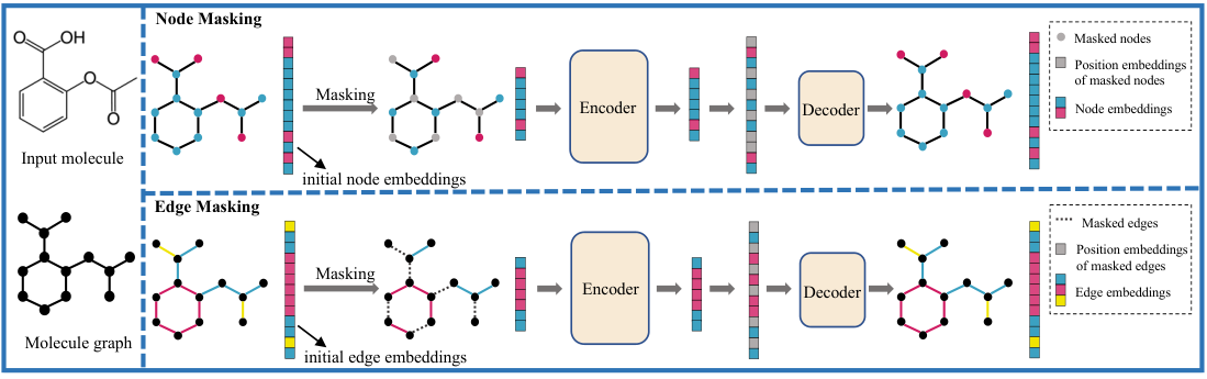
Refer to caption — Figure 1: Illustration of the designed self-supervised task of BatmanNet. A very high portion of nodes or edges is randomly masked, and then the BatmanNet is pre-trained to reconstruct the original molecule from the latent representation and mask tokens.

To address these challenges, we propose a novel molecular self-supervised framework, to alleviate the aforementioned issues and significantly improve the effectiveness and efficiency of molecular representation learning. First, we introduce a simple yet powerful self-supervised pre-training strategy. Instead of constructing complex pre-training tasks at multiple levels and introducing additional domain-specific chemical knowledge, our strategy is straightforward. We mask a high proportion ( $60\%$ ) of nodes and edges in the molecular graph, respectively, and reconstruct the missing parts through a graph-based autoencoder framework, as illustrated in Figure 1. This challenging self-supervised task enables our pre-training model to effectively and automatically learn both local and global information about molecular graphs, encouraging the acquisition of expressive structural and semantic knowledge of molecules in an end-to-end fashion. Compared to previous works rong2020self; li2021effective; li2022kpgt; fang2022geometry, our method is significantly more scalable and effective as it directly operates on the finest granularity of atoms and bonds. Second, we propose a simple, effective, and scalable form of bi-branch masked graph transformer autoencoder (BatmanNet) for molecular representation learning. Specifically, the encoder is a transformer-style architecture composed of multiple GNN-Attention blocks. The GNN is integrated into the attention layer to extract local and global information of molecular graphs, respectively. BatmanNet has an asymmetric encoder-decoder design. The encoder operates only on the visible subset of the molecular graph (without masked parts). The decoder reconstructs the molecular graph from the learned representation together with masked tokens, and its architecture is similar to the encoder but much more lightweight. With this asymmetrical design, the full set of molecular graphs is only processed by the lightweight decoder, which significantly reduces the amount of computation, the overall pre-training time, and memory consumption.

To verify the effectiveness of the proposed BatmanNet, we compared it with several state-of-the-art (SOTA) baselines on a wide range of downstream drug discovery tasks, including molecular properties prediction, drug-drug interaction prediction, and drug-target interaction prediction, with $13$ widely used benchmarks. The experimental results show that our BatmanNet performs much better on multiple drug discovery-related tasks, demonstrating the power capacity, effectiveness, and generalizability of BatmanNet.

In summary, our contributions are as follows:

•

We propose a novel self-supervised pre-training strategy for molecular representation learning to learn both local and global information of the molecules, masking nodes and edges simultaneously with a high mask ratio ( $60\%$ ) and reconstructing them via an autoencoder architecture.
•

We develop a bi-branch asymmetric graph-based autoencoder architecture, significantly enhancing the learning effectiveness and efficiency of the model and vastly reducing memory consumption.
•

We evaluated BatmanNet thoroughly on various drug discovery tasks. Experimental results demonstrate that BatmanNet outperforms competitive baselines on multiple benchmarks of drug discovery tasks.

2 Related Work

2.1 Molecular Representation Learning

Many efforts have been devoted to enhancing molecular representation learning to improve the performance of various downstream tasks involving molecules. Early feature-based approaches utilized fixed molecular representations, such as molecular descriptors and fingerprints, to represent molecules in vector spaces butler2018machine; dong2018admetlab; van2003admet. However, such methods heavily relied on complex feature engineering to achieve good predictive performance and suffered from vector sparsity issues.

In contrast to feature engineering-based representations, molecular representations learned through deep learning exhibit better generalization and higher expressiveness. Some studies coley2017convolutional; duvenaud2015convolutional introduced convolutional layers to learn the neural fingerprints of molecules and applied these neural fingerprints to downstream tasks like property prediction. Following these works, xu2017seq2seq employed SMILES representations as input and utilized RNN-based models to generate molecular representations. Some works use masked language modeling to pretrain BERT-style models (honda2019smiles; pesciullesi2020transfer; wang2019smiles; chithrananda2020chemberta) or use an autoencoder framework to reconstruct SMILES representations (winter2019learning; gomez2018automatic; xu2017seq2seq). However, the SMILES itself has several limitations in representing small molecules. First, it is not designed to capture molecular similarity, e.g., two molecules with similar chemical structures might be translated into markedly different SMILES strings, prone to misleading language models with the positional embedding (jin2018junction). Second, some essential chemical properties of molecules, such as molecular validity, are not readily expressed by the SMILES representation, resulting in more text sequences of invalid molecules. Recently, Graph Neural Networks (GNNs) have been widely applied in learning molecular graph representations, leveraging their significant advantages in modeling graph-structured data. For instance, some works kearnes2016molecular; schutt2017schnet; schutt2017quantum explored encoding molecular graphs into neural fingerprints using graph convolutional networks. Work by ryu2018deeply; xiong2019pushing proposed learning aggregation weights by extending the Graph Attention Network (GAT) velivckovic2017graph. To better capture interatomic interactions, gilmer2017neural introduced a message-passing framework, and gasteiger2020directional; yang2019analyzing extended this framework to model bond interactions. Additionally, lu2019molecular constructed a hierarchical GNN to capture multi-level interactions. While GNNs have made significant progress in the field of molecular graph representation learning, their use of message-passing operators aggregates only local information, making them incapable of capturing long-range dependencies within molecules.

2.2 Self-supervised Learning for Molecular Graphs

Self-supervised learning has a long history in machine learning and has yielded fruitful results in many fields, such as computer vision (he2022masked) and language modeling devlin2018bert. In light of this influence, self-supervised learning on molecular graphs has emerged as a core direction recently. Current self-supervised learning methods on molecular graphs can be further divided into two subgroups depending on the utilized molecular information level. One group of methods pre-trains $2$ D models from the molecular $2$ D topology li2021effective; hu2019strategies; rong2020self; li2022kpgt; liu2019n; chen2022graph; tan2022mgae. li2021effective; rong2020self; li2022kpgt all employ Transformer-style architectures to pre-train molecular graphs. In the case of li2021effective and rong2020self, motifs or subgraphs from molecules need to be predefined and extracted as prediction targets for their self-supervised tasks. li2022kpgt, on the other hand, requires the introduction of additional knowledge, with random masking of a certain proportion of the additional knowledge as part of the reconstruction target. In contrast, our proposed self-supervised learning strategy involves a simple bi-branch graph-masking task that doesn’t require specific domain knowledge, such as predefined motifs, subgraphs, or additional information. It is more straightforward, intuitive, and easier to implement. Furthermore, our approach involves the random masking of a high proportion of nodes and edges, each node and edge embedding must learn local contextual information, and the model also needs to learn global information to predict the entire graph from the remaining subgraphs. This makes our task more challenging compared to other self-supervised pretraining tasks. The pre-training models in works li2021effective; rong2020self; li2022kpgt are all constructed based on the Transformer architecture, resulting in a large number of model parameters and high computational complexity, necessitating significant computational resources. In contrast, our BatmanNet utilizes an asymmetric transformer-style autoencoder, substantially reducing the model’s parameter count and computational complexity, thereby further enhancing the efficiency of our approach. The other methods worked on the $3$ D geometry graphs with spatial positions of atoms by utilizing geometric GNN models (liu2021pre; fang2022geometry). Although graph-based methods explicitly consider molecular structural information, they usually require a large volume of molecule data for pre-training due to their complicated architectures, which may limit their generalization abilities when the data is sparse.

Among the graph-based methods, GMAE chen2022graph, MGAE tan2022mgae, and GraphMAE hou2022graphmae are the most relevant to our work. However, unlike GMAE masking nodes only and MGAE masking edges only, BatmanNet constructs a bi-branch complementary autoencoder. The dual branches perform node masking and edge masking, respectively, to enhance the expressiveness of the model. GraphMAE is designed to replace masked nodes with descriptors. In contrast, our method directly removes the masked part and adopts two branches to mask nodes and edges, respectively. The learning task in our approach is more challenging than that in GraphMAE, resulting in a more capable model. Therefore, we believe that our architecture and self-supervised learning strategy are a superior choice for molecular representation learning compared to other methods.

3 Materials and methods

3.1 Preliminaries

Graph Neural Networks (GNNs). GNNs are a class of neural networks designed for graph-structured data, and they have been successfully applied in a broad range of domains. One of the key components of most GNNs is the message passing (also called neighborhood aggregation) mechanism between nodes in the graph, where the hidden representation $\mathbf{h}_{v}$ of node $v$ is iteratively updated by aggregating the states of the neighboring nodes and edges. For a GNN with $K$ layers, repeating the message passing by $K$ times, the $v$ ’s hidden representation will contain the structural information of $K$ -hop on the graph topology. Formally, the $k$ -th layer of a GNN can be formulated as,

\mathbf{m}_{v}^{(k)}=\operatorname{AGG}^{(k)}\left(\left\{\left(\mathbf{h}_{v}^{(k-1)},\mathbf{h}_{u}^{(k-1)},\mathbf{e}_{uv}\right)\mid u\in\mathcal{N}_{v}\right\}\right),

(1)

\mathbf{h}_{v}^{(k)}=\sigma\left(\mathbf{W}^{(k)}\mathbf{m}_{v}^{(k)}+\mathbf{b}^{(k)}\right),

(2)

where $\mathbf{m}_{v}^{(k)}$ is the aggregated message, $\mathbf{h}_{v}^{(k)}$ is the representation of node $v$ at the $k$ -th layer, $\mathbf{e}_{uv}$ is the representation of edge $(u,v)$ , $\sigma(\cdot)$ is the activation function, and $\mathcal{N}_{v}$ is a set neighbors of $v$ . $\operatorname{AGG}^{(k)}(\cdot)$ is the neighborhood aggregation process of the $k$ -th layer. For convenience, we initialize $\mathbf{h}_{v}^{(0)}=X_{v}$ . After the final iteration $K$ , a READOUT function is applied to get the entire graph’s representation $\mathbf{h}_{G}$ ,

\mathbf{h}_{G}=\operatorname{READOUT}\left(\left\{\mathbf{h}_{v}^{\left(K\right)}\mid v\in\mathcal{V}\right\}\right),

(3)

where $\mathcal{V}$ is the set of nodes (atoms).

Multi-head attention mechanism. The multi-head attention mechanism is the core building block of Transformer vaswani2017attention with several stacked scaled dot-product attention layers. The input of the scaled dot-product attention layer consists of queries $\mathbf{q}$ and keys $\mathbf{k}$ with dimension $d_{k}$ and values $\mathbf{v}$ of dimension $d_{v}$ . In practice, the set of ( $\mathbf{q}$ , $\mathbf{k}$ , $\mathbf{v}$ )s are packed together into matrices ( $\mathbf{Q}$ , $\mathbf{K}$ , $\mathbf{V}$ ) so that they can be computed simultaneously. The final output matrix is computed by,

\operatorname{Attention}(\mathbf{Q},\mathbf{K},\mathbf{V})=\operatorname{softmax}\left(\frac{\mathbf{Q}\mathbf{K}^{T}}{\sqrt{d_{k}}}\right)\mathbf{V}.

(4)

Multi-head attention allows the model to focus jointly on information from different representation subspaces. Suppose multi-head attention has $h$ parallel attention layers, then the output is,

\operatorname{MultiHead}(\mathbf{Q},\mathbf{K},\mathbf{V})=\operatorname{Concat}\left(\operatorname{head}_{1},\ldots,\text{head}_{h}\right)\mathbf{W}^{O},

(5)

\text{head}_{i}=\operatorname{Attention}\left(\mathbf{Q}\mathbf{W}_{i}^{\mathbf{Q}},\mathbf{K}\mathbf{W}_{i}^{\mathbf{K}},\mathbf{VW}_{i}^{\mathbf{V}}\right),

(6)

where $\mathbf{W}_{i}^{\mathbf{Q}},\mathbf{W}_{i}^{\mathbf{K}},\mathbf{W}_{i}^{\mathbf{V}}$ are projection weights of head $i$ .

Figure 2: Overview of the BatmanNet architecture with node-branch (left) and edge-branch (right). The bottom sub-network colored light orange is BatmanNet’s encoder. After pre-training, it will be used as a feature extractor for the downstream molecular property prediction tasks by stacking two MLPs on top of two branches, and the final prediction is averaged over the two outputs. The upper sub-network colored light blue is BatmanNet’s decoder.

3.2 Overview of BatmanNet

This section describes our proposed bi-branch masked graph transformer autoencoder for molecular representation learning (BatmanNet), including the BatmanNet framework and the self-supervised pre-training strategy.

3.2.1 The BatmanNet framework

As depicted in Figure 2, BatmanNet is a bi-branch model with a node and an edge branch. Each branch focuses on learning the embeddings of nodes or edges from the input graph for fine-tuning downstream tasks. Similar to MAE (he2022masked), we propose a transformer-style asymmetric encoder-decoder architecture for each branch. By applying a bi-branch graph masking pre-training strategy, the encoder operates on partially observable signals of molecular graphs and embeds them into latent representations of nodes or edges. The lightweight decoder takes the latent representations of nodes and edges along with mask tokens to reconstruct the original molecule.

For a molecule, we denote the set of nodes (atoms) as $V$ and the set of edges (bonds) as $E$ . We introduce node graph $G_{N}$ and edge graph $G_{E}$ for each molecule. The node graph is defined as $G_{N}=(V,E)$ , where atom $v\in V$ is regarded as the node of $G_{N}$ and bond $(u,v)\in E$ as the edge of $G_{N}$ , connecting atoms $u$ and $v$ . The initial features of nodes and edges are denoted by $X_{v}$ and $e_{u}{}_{v}$ , respectively. We can apply GNNs to the node graph to perform the message passing over nodes. The edge graph $G_{E}$ is the primary dual of the node graph, describing the neighboring edges in the original graph and ensuring message passing over edges in a similar fashion (chen2017supervised). The node graph $G_{N}$ and the edge graph $G_{E}$ are taken as the inputs of the node branch and edge branch of BatmanNet, respectively.

As shown in Figure 2, the encoder consists of two symmetric multi-layer transformer-styled networks based on the implementation described in (rong2020self), mapping the initial features of visible, unmasked nodes and edges to embeddings in their latent feature spaces. The decoder takes the input of a complete set of reordered molecular representations, including (i) the embeddings of unmasked nodes and edges from the encoder and (ii) mask tokens of removed nodes and edges. The decoder uses the same transformer-styled architecture as the encoder but is more lightweight, and it is only used in the pre-training stage to perform the molecular reconstruction task. Only the encoder is used to produce molecular representations for the downstream tasks. Based on (he2022masked), a narrower or shallower decoder would not impact the overall performance of the MAE. In this asymmetric encoder-decoder design, the nodes and edges of the entire graph are only processed at the lightweight decoder. This significantly reduces the model’s computation and memory consumption pre-training.

Details of encoder and decoder. As illustrated in Figure 2, The encoder and decoder consist of a stack of $N$ and $M$ ( $M\ll N$ ) identical layers of the GNN-Attention block, respectively, with each block adopting a double-layer information extraction framework. The GNN is integrated into the attention layer to extract local and global information of molecular graphs, respectively.

In a GNN-Attention block, a GNN is used as the first layer of the information extraction network. It performs the message passing operation on the input graph to extract local information, and the output is the learned embeddings. A multi-head attention layer is then employed to capture the global information of the graph. Specifically, a GNN-Attention block comprises three GNNs, i.e., $\mathbf{G}_{\mathbf{Q}}(\cdot),\mathbf{G}_{\mathbf{K}}(\cdot)$ , and $\mathbf{G}_{\mathbf{V}}(\cdot)$ , that learn embedding of queries $\mathbf{Q}$ , keys $\mathbf{K}$ , and values $\mathbf{V}$ as follows:

\mathbf{Q}=\mathbf{G}_{\mathbf{Q}}(\mathbf{H}),

(7)

\mathbf{K}=\mathbf{G}_{\mathbf{K}}(\mathbf{H}),

(8)

\mathbf{V}=\mathbf{G}_{\mathbf{V}}(\mathbf{H}),

(9)

where $\mathbf{H}\in\mathbb{R}^{n\times d}$ is the hidden representation matrix of $n$ nodes, with an embedding size of $d$ . Then we apply equations (4), (5), and (6) to obtain the final output of the GNN-Attention block.

At the beginning of the encoder, we use a linear projection with added positional embeddings to preserve the positional information of unmasked nodes and edges. Here we adopt the absolute sinusoidal positional encoding proposed by vaswani2017attention, and the positions of nodes and edges in the input graph are indexed by RDkit before masking. By feeding the original graph and its dual graph to both branches of the encoder, respectively, we get the aggregated node embedding $\mathbf{m}_{v}$ and edge embedding $\mathbf{m}_{vw}$ as follows:

\mathbf{m}_{v}=\sum_{u\in\mathcal{N}_{v}}\mathbf{h}_{u},

(10)

\mathbf{m}_{vw}=\sum_{u\in\mathcal{N}_{v}\backslash w}\mathbf{h}_{uv}.

(11)

We add long-range residual connections from the initial features of nodes and edges to $\mathbf{m}_{v}$ and $\mathbf{m}_{vw}$ to overcome the vanishing gradient and alleviate over-smoothing at the message passing stage. In the last step, we apply a Feed Forward and LayerNorm to obtain the unmasked node embedding and edge embedding as the final output of the encoder.

At the beginning of the decoder, we first use a Feature Reordering layer (as shown in Figure 2) that concatenates the embeddings of unmasked nodes and edges from the encoder and masked tokens of removed nodes and edges, recovering their order in original input graphs by adding corresponding positional embeddings. Afterwards, the decoder uses the same transformer-styled architecture as the encoder to obtain the node embedding and edge embedding.

Reconstruction Target. BatmanNet’s node and edge branches reconstruct molecules by predicting all features of masked nodes and edges, respectively. The features of node (atom) and edge (bond) we used in BatmanNet are referred to in Supplementary Section 2.1. A linear layer is appended to each decoder’s output, and its output dimension is set as the total amount of the feature size of either atoms (for node branch) or bonds (for edge branch). Both the reconstruction tasks of nodes and edges involve high-dimension multi-label predictions, which can alleviate the ambiguity problem discussed by (rong2020self) where a limited number of the atom or edge types are used as the node/edge level pre-training targets. The pre-training loss is computed on the masked tokens similar to MAE (he2022masked), and the final pre-training loss $\mathcal{L}_{\text{pre-train}}$ is defined as:

\mathcal{L}_{\text{pre-train}}=\mathcal{L}_{\text{node}}+\mathcal{L}_{\text{edge}},

(12)

\mathcal{L}_{\text{node}}=\sum_{v\in\mathcal{V}_{\text{mask}}}\mathcal{L}_{\text{ce}}\left(\boldsymbol{p}_{v},\boldsymbol{y}_{v}\right),

(13)

\mathcal{L}_{\text{edge}}=\sum_{(u,v)\in\mathcal{E}_{\text{mask}}}\mathcal{L}_{\text{ce}}\left(\boldsymbol{p}_{(u,v)},\boldsymbol{y}_{(u,v)}\right),

(14)

where $\mathcal{L}_{\text{node}}$ and $\mathcal{L}_{\text{edge}}$ are the loss functions of the node branch and edge branch. $\mathcal{V}_{\text{mask}}$ and $\mathcal{E}_{\text{mask}}$ represent the set of masked nodes and edges, respectively. $\mathcal{L}_{\text{ce}}$ is the cross entropy loss between predicted node features $\boldsymbol{p}_{v}$ and corresponding ground-truth $\boldsymbol{y}_{v}$ or predicted edge features $\boldsymbol{p}_{(u,v)}$ and corresponding ground-truth $\boldsymbol{y}_{(u,v)}$ .

3.2.2 Pre-training strategy: Bi-branch graph masking

The efficacy of a pre-trained model heavily relies on the design of self-supervision tasks, which should ideally encompass both node and graph levels to enable the model to learn local and global molecular graph information (li2021effective; hu2019strategies; rong2020self; fang2022geometry). Inspired by MAE (he2022masked), we propose a self-supervised pre-training strategy that accomplishes this goal through a single prediction task, using a bi-branch graph masking and reconstruction approach for molecular pre-training. Specifically, given a molecular graph, our approach randomly masks a high proportion of its nodes and edges in both the node and edge branches of the model. The encoder then operates on the remaining unmasked nodes and edges. It is worth mentioning that, considering that the message passing process in GNNs is directed, we adopt the directed masking scheme (tan2022mgae) to the random masking of edges (i.e., $(u,v)$ and $(v,u)$ are different). Removing $(u,v)$ does not mean that $(v,u)$ is also removed. To distinguish $(u,v)$ and $(v,u)$ , we add the feature of the starting node (head node) to the initial feature of the edge.

Our design of the strategy is effective for two reasons. First, our node-level pre-training approach enables the learning of local contextual information beyond the k-hops range and limited shapes. Previous node/edge-level pre-training strategies typically rely on multiple prediction tasks to capture domain knowledge by learning neighboring graph structures and the regularities of the node/edge attributes distributed over these graph structures (hu2019strategies) or introducing additional definitions such as motifs rong2020self, subgraphs li2021effective, and additional knowledge li2022kpgt. In contrast, our approach randomly masks a high percentage of nodes and edges, e.g., $60\%$ , so that each node/edge has a high likelihood of missing neighboring nodes and edges simultaneously. To reconstruct the missing neighboring nodes and edges, each node and edge embedding must learn its contextual information locally. This high ratio of random masking and reconstruction removes the restriction of scale and shape of subgraphs used for prediction, thus promoting the capturing of local contextual information beyond the k-hops range and limited shapes. Second, our graph-level pre-training approach involves predicting the entire graph from the remaining nodes and edges after random masking, resulting in a more challenging task than other self-supervised pre-training tasks that typically learn global graph information with smaller graphs or motifs as the target (rong2020self; li2021effective). This more challenging pre-training task of bi-branch graph masking and reconstruction entails a more powerful model with a larger capacity for learning high-quality node and edge embeddings to capture molecular information at both the local and global levels.

Overall, our proposed pre-training strategy achieves a more efficient and effective learning of molecular information at both the node/edge and graph levels while maintaining the learning capacity of the pre-training tasks.

{sidewaystable*}

[htbp] Overall performance for classification tasks and regression tasks of molecular properties prediction. Methods Classification (AUC-ROC) Regression (RMSE) Dataset BACE BBBP ClinTox SIDER Tox21 ToxCast FreeSolv ESOL Lipo #Molecules 1513 2039 1478 1427 7831 8575 642 1128 4200 #tasks 1 1 2 27 12 617 1 1 1 ECFP (rogers2010extended) 0.861_(0.024) 0.783_(0.050) 0.673_(0.031) 0.630_(0.019) 0.760_(0.009) 0.615_(0.017) 5.275_(0.751) 2.359_(0.454) 1.188_(0.061) TF_Robust (ramsundar2015massively) 0.824_(0.022) 0.860_(0.087) 0.765_(0.085) 0.607_(0.033) 0.698_(0.012) 0.585_(0.031) 4.122_(0.085) 1.722_(0.038) 0.909_(0.060) GraphConv (kipf2016semi) 0.854_(0.011) 0.877_(0.036) 0.845_(0.051) 0.593_(0.035) 0.772_(0.041) 0.650_(0.025) 2.900_(0.135) 1.068_(0.050) 0.712_(0.049) Weave (kearnes2016molecular) 0.791_(0.008) 0.837_(0.065) 0.823_(0.023) 0.543_(0.034) 0.741_(0.044) 0.678_(0.024) 2.398_(0.250) 1.158_(0.055) 0.813_(0.042) SchNet (schutt2017schnet) 0.750_(0.033) 0.847_(0.024) 0.717_(0.042) 0.545_(0.038) 0.767_(0.025) 0.679_(0.021) 3.215_(0.755) 1.045_(0.064) 0.909_(0.098) MPNN (gilmer2017neural) 0.815_(0.044) 0.913_(0.041) 0.879_(0.054) 0.595_(0.030) 0.808_(0.024) 0.691_(0.013) 2.185_(0.952) 1.167_(0.430) 0.672_(0.051) DMPNN (yang2019analyzing) 0.852_(0.053) 0.919_(0.030) 0.897_(0.040) 0.632_(0.023) 0.826_(0.023) 0.718_(0.011) 2.177_(0.914) 0.980_(0.258) 0.653_(0.046) MGCN (lu2019molecular) 0.734_(0.030) 0.850_(0.064) 0.634_(0.042) 0.552_(0.018) 0.707_(0.016) 0.663_(0.009) 3.349_(0.097) 1.266_(0.147) 1.113_(0.041) AttentiveFP (xiong2019pushing) 0.863_(0.015) 0.908_(0.050) 0.933_(0.020) 0.605_(0.060) 0.807_(0.020) 0.579_(0.001) 2.030_(0.420) 0.853_(0.060) 0.650_(0.030) TrimNet (li2021trimnet) 0.843_(0.025) 0.892_(0.025) 0.906_(0.017) 0.606_(0.006) 0.812_(0.019) 0.652_(0.032) 2.529_(0.111) 1.282_(0.029) 0.702_(0.008) Mol2Vec (jaeger2018mol2vec) 0.841_(0.052) 0.876_(0.030) 0.828_(0.023) 0.601_(0.023) 0.805_(0.015) 0.690_(0.052) 5.752_(1.245) 2.358_(0.452) 1.178_(0.054) N-GRAM (liu2019n) 0.876_(0.035) 0.912_(0.013) 0.855_(0.037) 0.632_(0.005) 0.769_(0.027) - 2.512_(0.190) 1.100_(0.160) 0.876_(0.033) SMILES-BERT (wang2019smiles) 0.849_(0.021) 0.959 ${}_{\textbf{(0.009)}}$ 0.985 ${}_{\textbf{(0.014)}}$ 0.568_(0.031) 0.803_(0.010) 0.665_(0.010) 2.974_(0.510) 0.841_(0.096) 0.666_(0.029) pre-trainGNN (hu2019strategies) 0.851_(0.027) 0.915_(0.040) 0.762_(0.058) 0.614_(0.006) 0.811_(0.015) 0.714_(0.019) - - - GraphMAE¹¹footnotemark: 1 (hou2022graphmae) 0.863_(0.002) 0.896_(0.007) 0.850_(0.007) 0.652_(0.001) 0.794_(0.003) 0.679_(0.005) - - - GROVERbase (rong2020self) 0.878_(0.016) 0.936_(0.008) 0.925_(0.013) 0.656_(0.023) 0.819_(0.020) 0.723_(0.010) 1.592_(0.072) 0.888_(0.116) 0.563_(0.030) GROVERlarge (rong2020self) 0.894_(0.028) 0.940_(0.019) 0.944_(0.021) 0.658_(0.023) 0.831_(0.025) 0.737_(0.010) 1.544_(0.397) 0.831_(0.120) 0.560_(0.035) KPGT (li2022kpgt) 0.855_(0.011) 0.908_(0.010) 0.946_(0.022) 0.649_(0.009) 0.848_(0.013) 0.746_(0.002) 2.121_(0.837) 0.803_(0.008) 0.600_(0.010) MPG (li2021effective) 0.920_(0.013) 0.922_(0.012) 0.963_(0.028) 0.661_(0.007) 0.837_(0.019) 0.748_(0.005) 1.269_(0.192) 0.741_(0.017) 0.556 ${}_{\textbf{(0.017)}}$ GEM (fang2022geometry) 0.925_(0.010) 0.953_(0.007) 0.977_(0.019) 0.663_(0.014) 0.849_(0.003) 0.742_(0.004) - - - BatmanNet 0.928 ${}_{\textbf{(0.008)}}$ 0.946_(0.003) 0.926_(0.002) 0.676 ${}_{\textbf{(0.007)}}$ 0.855 ${}_{\textbf{(0.005)}}$ 0.756 ${}_{\textbf{(0.007)}}$ 1.174 ${}_{\textbf{(0.054)}}$ 0.736 ${}_{\textbf{(0.014)}}$ 0.578_(0.034) \botrule {tablenotes}

The methods in shading cells are pre-trained methods. The SOTA results are shown in bold. Standard deviations are in brackets.

To offer a fair comparison, we re-tested GraphMAE(hou2022graphmae) under the same experimental conditions as MPG(li2021effective).

4 Experiments and Results

To comprehensively evaluate the performance of BatmanNet, we conduct extensive experiments and compare its performance against several SOTA methods across multiple benchmarks. These benchmarks encompass a wide range of molecular property prediction tasks, including those related to physical, chemical, and biophysical properties, as well as drug-drug interaction (DDI) and drug-target interaction (DTI) prediction tasks.

4.1 Pre-training settings

4.1.1 Pre-training Datasets.

The pre-training of BatmanNet is carried out on the ZINC- $250$ K molecule dataset from kusner2017grammar. The dataset is composed of $250$ K molecules that were sampled from the ZINC database sterling2015zinc. Here we randomly split the dataset into training and validation sets in a $9:1$ ratio.

4.1.2 Experimental Configurations.

We use the Adam (kingma2014adam) optimizer and the Noam learning rate scheduler (devlin2018bert) to optimize the model and adjust the learning rate for pre-train. The batch size is set as $32$ , and the BatmanNet is implemented by PyTorch NEURIPS2019_9015. The masking ratio for both branches of BatmanNet is set as $0.6$ , while the encoder and decoder consist of $6$ and $2$ layers, respectively, with a hidden size of $100$ . The GNN-attention block of each layer utilizes $3$ GNN layers and $2$ self-attention heads. The autoencoder structure comprises roughly $2.6M$ parameters and is pre-trained for two days on a single Nvidia RTX3090.

4.1.3 Pre-trained representations visualization.

In order to visually observe the representations that the self-supervised tasks (without downstream fine-tuning) have learned, we projected them into a two-dimensional space for visualization purposes. Here, we investigated whether the pre-training method is able to effectively discriminate between molecules with valid structures and those with invalid structures. We randomly selected 1,500 molecules with valid structures from the ZINC dataset and introduced structural perturbations to generate invalid molecules by shuffling atom features and altering the order of atoms and bonds. For each valid and invalid molecule, we extracted the embedding from the last layer of the pre-trained BatmanNet as molecular representations. Subsequently, we employed the UMAP algorithm mcinnes2018umap to map these representations into a two-dimensional space for visualization. We also conducted a similar analysis on the BatmanNet model that was not pre-trained for comparison. As illustrated in Figure 3(a) and 3(b), in comparison to the not pre-trained model, the pre-trained BatmanNet demonstrates an enhanced ability to distinguish between molecules with valid structures and those with invalid structures, suggesting that pre-trained models can effectively discern the structural validity of molecules.

4.2 Molecular property prediction settings.

4.2.1 Datasets.

To assess the efficacy of pre-trained BatmanNet in predicting molecular properties, we conducted experiments on several benchmark datasets from MoleculeNet wu2018moleculenet. These datasets encompass both classification and regression tasks, and additional information about the datasets may be found in Supplementary Section 1.1. Following the previous worksrong2020self; li2021effective; fang2022geometry, We apply scaffold splitting (bemis1996properties; ramsundar2019deep) to split the dataset into training, validation, and test sets at a ratio of $8:1:1$ in each downstream task. This approach segregates the dataset into various substructures, enabling the evaluation of the model’s ability to generalize outside of the distribution, a challenging yet reliable evaluation. More details are deferred to Supplementary Section 2.

4.2.2 Baselines.

We compare the performance of BatmanNet with $20$ competitive baselines for molecular property prediction. We evaluate $10$ supervised learning models without pre-training, i.e., ECFP (rogers2010extended), TF_Robust (ramsundar2015massively), GraphConv (kipf2016semi), Weave (kearnes2016molecular), SchNet (schutt2017schnet), MPNN (gilmer2017neural), DMPNN (yang2019analyzing), MGCN (lu2019molecular), AttentiveFP (xiong2019pushing) and TrimNet (li2021trimnet), and $10$ self-supervised learning models with pre-training, i.e., Mol2Vec (jaeger2018mol2vec), N-GRAM (liu2019n), SMILES-BERT (wang2019smiles), pre-trainGNN (hu2019strategies), GraphMAE (hou2022graphmae), $\text{GROVER}_{\text{base}}$ , $\text{GROVER}_{\text{large}}$ (rong2020self), KPGT li2022kpgt, MPG (li2021effective), and GEM (fang2022geometry). Among them, ECFP is a circular topological fingerprint designed for molecular characterization, similarity searching, and structure-activity modeling. TF_Roubust is a DNN-based multi-task framework that takes molecular fingerprints as input. GraphConv, Weave, and SchNet are three graph convolution models. MPNN and its variants DMPNN and MGCN are models considering edge features during message passing. AttentiveFP is an extension of the graph attention network. TrimNet is a graph-based approach and employs a novel triplet message mechanism to learn molecular representation efficiently. Mol2Vec, N-GRAM, and SMILES-BERT are inspired by NLP approaches to pre-train a model on sequential representation. pre-trainGNN, GraphMAE, GROVER, and MPG are graph-based pre-training models with various pre-training strategies. KPGT is a knowledge-guided pre-training method based on the graph transformer. GEM is a geometry-based graph neural network architecture with several dedicated geometry-level self-supervised learning strategies to learn molecular geometry knowledge. We only report classification results for pre-trainGNN, GraphMAE, and GEM since the original implementation does not admit regression tasks without non-trivial modifications.

4.2.3 Experimental configurations and Evaluation metrics.

In order to ensure a fair comparison, we adopted the experimental setup used in previous SOTA methods—GROVER rong2020self, MPG li2021effective, and GEM fang2022geometry (Section 4.1 of GEM’s Supplementary Information). We selected the model with the best performance on the validation set. Three independent runs were conducted for each property prediction task, and we reported the mean and standard deviation of the ROC-AUC or RMSE. Further pre-training and fine-tuning details are deferred to Supplementary Section 2.

4.2.4 Experimental results.

Table 3.2.2 summarizes the performance of BatmanNet along with previous supervised and self-supervised methods on molecular properties prediction. Our results demonstrate that BatmanNet achieves state-of-the-art performance on 6 out of 9 datasets. Compared to molecular fingerprint and supervised models without pre-training, BatmanNet significantly outperforms them on all datasets. On the classification tasks, BatmanNet exceeds the previous SOTA model—GEM on $4$ out of $6$ datasets. On the regression tasks, BatmanNet outperforms the previous SOTA model—MPG on $2$ out of $3$ datasets.

Figure 4: Efficacy and Effectiveness Analysis. The figure illustrates the pre-training dataset size and model size for BatmanNet and a series of advanced baselines, along with their average AUC across all classification datasets about molecular property prediction. The horizontal axis represents the dataset size, the vertical axis represents the average AUC, the circle size corresponds to the model size, and the diamond indicates that the size of the model is unknown.

4.2.5 Efficacy and Effectiveness Analysis.

As illustrated in Figure 4, we conducted a further analysis of the pre-training dataset size and model size for BatmanNet and a series of advanced baselines. We compared their average AUC across all classification datasets about molecular property prediction, see Supplementary Table S4. The results reveal that BatmanNet achieves comparable performance to the previously state-of-the-art models while utilizing fewer training data and model parameters. This finding substantiates the superior efficacy and efficiency of our proposed method.

Table 1: DDI prediction performance of BatmanNet and other various baselines on BIOSNAP dataset

Model	AUC-ROC	PR-AUC	F1
LR	0.802_(0.001)	0.779_(0.001)	0.741_(0.002)
Nat.Prot vilar2014similarity	0.853_(0.001)	0.848_(0.001)	0.714_(0.001)
Mol2Vec jaeger2018mol2vec	0.879_(0.006)	0.861_(0.005)	0.798_(0.007)
MolVAE gomez2018automatic	0.892_(0.009)	0.877_(0.009)	0.788_(0.033)
DeepDDI (ryu2018deep)	0.886_(0.007)	0.871_(0.007)	0.817_(0.007)
CASTER huang2020caster	0.910_(0.005)	0.887_(0.008)	0.843_(0.005)
GEM fang2022geometry	0.960_(0.003)	0.956_(0.002)	0.903_(0.003)
MPG li2021effective	0.966_(0.004)	0.960_(0.004)	0.905_(0.008)
BatmanNet	0.972 ${}_{\textbf{(0.001)}}$	0.966 ${}_{\textbf{(0.001)}}$	0.916 ${}_{\textbf{(0.002)}}$
\botrule

{tablenotes}

The dataset was divided into training/validation/testing sets in a 7:1:2 ratio. The mean and standard deviation of performances run with three random seeds are reported.

Table 2: DTI prediction performance of BatmanNet and other various baselines on Human and C. elegans dataset.

Datasets	Model	Precision	Precision	AUC
	Tsubaki et al. tsubaki2019compound	0.923	0.918	0.970
	GEM fang2022geometry	0.930	0.930	0.972
Human	MPG li2021effective	0.952	0.940	0.985
	BatmanNet	0.983	0.982	0.998
	(Relative improvement)	(3.26%)	(4.47%)	(1.32%)
	Tsubaki et al. tsubaki2019compound	0.938	0.929	0.978
	GEM fang2022geometry	0.955	0.954	0.988
C.elegans	MPG li2021effective	0.954	0.959	0.986
	BatmanNet	0.988	0.987	0.999
	(Relative improvement)	(3.46%)	(2.92%)	(1.11%)
\botrule

Table 3: 5-fold cross-validation DDI prediction performance of BatmanNet and various other baselines on the TWOSIDES dataset, and the results show that BatmanNet outperforms other baselines.

Model	Precision	Recall	F1
DDI_PULearn zheng2019ddi	0.904	0.824	0.862
GEM fang2022geometry	0.928	0.929	0.928
MPG li2021effective	0.936	0.936	0.936
BatmanNet	0.939	0.939	0.939
\botrule

4.3 Drug-drug interaction prediction settings.

To assess the effectiveness of BatmanNet on DDI prediction tasks, we formulate the problem as a binary classification task, aiming to predict whether two drugs are likely to interact. Following the approach of MPG (li2021effective), we compared BatmanNet against recently proposed methods on two real-world datasets—BIOSNAP (zitnik2018biosnap) and TWOSIDES (tatonetti2012data) (For details about both datasets, refer to Supplementary Section 1.1). To ensure a fair comparison, we followed the same experimental procedure as the best approaches—MPG (li2021effective) on the aforementioned datasets. Additionally, to compare with the previous best molecular self-supervised learning model—GEM (fang2022geometry), we fine-tuned GEM on the two DDI prediction datasets under the same experimental conditions. Classification results are reported in Table 1 and Table 3. All baselines, except GEM, are taken from MPG. Results in Table 1 and Table 3 indicate that BatmanNet outperforms the previous state-of-the-art method (MPG) on both datasets. These findings demonstrate the superior performance of our BatmanNet on DDI prediction tasks.

4.4 Drug-target interaction prediction settings.

Drug-target interaction (DTI) prediction is a critical task in the field of AI-assisted drug discovery (AIDD), aimed at identifying the interaction between a compound and a target protein for drug discovery. Deep learning algorithms have been widely employed for DTI prediction, typically involving encoding compounds and proteins separately. Tsubaki et al. (tsubaki2019compound) proposed a new DTI prediction framework, using GNNs to encode compounds and CNNs to encode proteins. Another recent approach, proposed by Li et al. (li2021effective), utilized a pre-trained MolGNet as the compound encoder, achieving superior performance compared to existing methods. In this study, we modified the DTI prediction framework proposed by Tsubaki et al. (tsubaki2019compound), replacing their compound encoder with our pre-trained BatmanNet to assess its effectiveness. To ensure a fair comparison, we adopted the same experimental procedure as MPG (li2021effective) and evaluated our model on two widely used datasets, namely the Human and C. elegans datasets (Details about both datasets are available in Supplementary Section 1.1). Moreover, to compare the performance of GEM (fang2022geometry) on the DTI prediction task, we employed GEM as the compound encoder and fine-tuned it on the same two datasets. Results, as shown in Table 2, demonstrate a significant improvement in performance on both datasets when using BatmanNet as the compound encoder, with increases in the precision of 3.26% and 3.46%, respectively, compared to the previous best model—MPG (li2021effective). The results indicate the strong transfer learning capabilities of BatmanNet in molecular representation learning, offering promising prospects for its use in future DTI prediction research.

Figure 5: Ablation studies. (a), Comparison between BatmanNet with bi-branch and with a single branch (only node or edge branch) on classification tasks of molecular property prediction. (b), Comparison results of the pre-trained BaemanNet and the BatmanNet without pre-training on classification tasks of molecular property prediction. (c), Comparison of different masking ratios. The y-axis is the average AUC on all classification datasets about molecular property prediction in this paper.

4.5 Ablation studies.

To delve deeper into the factors influencing the performance of our proposed BatmanNet framework, we conducted ablation studies on 6 classification benchmarks about molecular property prediction.

Effectiveness of the Bi-branch Information Extraction Network. To assess the impact of the bi-branch design in BatmanNet, we conducted an ablation study by replacing the bi-branch information extraction network with a single-branch network, either the node branch or the edge branch. Both single-branch networks were pre-trained under the same conditions as the bi-branch network and had nearly the same size of parameters ( $2.6M$ ). Figure 5(a) shows that using the bi-branch design in BatmanNet improves the average AUC by $2.9\%$ and $3.0\%$ compared to using only the node branch or edge branch, respectively, indicating the effectiveness of the bi-branch design.

Impact of the Self-Supervised Pre-training Strategy. To evaluate the influence of our self-supervised learning strategy, we compared the classification performance of pre-trained BatmanNet and BatmanNet without pre-training on molecular property prediction tasks using the same hyperparameters. As reported in Figure 5(b), the pre-trained model consistently outperforms the non-pre-trained model, with an average AUC improvement of $4.0\%$ . These findings indicate that our self-supervised pre-training strategy effectively captures rich structural and semantic information about molecules, leading to performance improvement in downstream tasks.

Effect of Different Masking Ratio. To examine the impact of different masking ratios, we conducted a study to pre-train BatmanNet with masking ratios ranging from $10\%$ to $90\%$ , then measured the average AUC in all downstream tasks. The detailed results of this study are available in Supplementary Section 3.2, while Figure 5(c) provides an overview of our findings. We observed that setting the masking ratio to $60\%$ led to the best performance. These results suggest that when a relatively high masking ratio is used, nodes and edges are masked with a greater frequency, resulting in a more challenging pre-training task. This challenging task provides a larger capacity for remaining nodes and edges to capture molecular information in their embeddings. However, when the masking ratio was set higher than $60\%$ , there was not enough information in the remaining nodes and edges to recover the complete graph. As a result, the quality of learned embeddings started to decline.

5 Discussion

Effective molecular representation learning holds significant importance in the field of AIDD and plays a crucial role in various downstream tasks involving molecules. In this paper, we address two major challenges in current self-supervised learning methods for molecular graphs: complex pre-training tasks and high computational complexity with large model sizes. We introduce a novel self-supervised learning framework for molecular representation learning, consisting of the bi-branch masked graph transformer autoencoder (BatmanNet) and a bi-branch graph masking self-supervised learning strategy. This framework aims to mitigate the mentioned issues, facilitating the learning of more generalizable, transferable, and robust representations of molecular graphs. Extensive test results demonstrate that BatmanNet outperforms current state-of-the-art methods across multiple molecular downstream task datasets.

Our approach offers advantages over several previously advanced methods. First, prior work on molecular self-supervised learning often required constructing multiple tasks to learn local and global information about molecules hu2019strategies; rong2020self; li2021effective; fang2022geometry, along with the need of predefined additional domain knowledge, such as motifs rong2020self, subgraphs li2021effective, the atomic distance matrix fang2022geometry, or additional knowledge li2022kpgt. Our method only necessitates a simple bi-branch graph masking task combined with a customized pre-training architecture (BatmanNet) to simultaneously learn local and global information about molecules, without requiring additional domain knowledge. This makes our method more scalable and easily applicable to larger pre-training datasets, enhancing the generalization ability of the pre-trained model. It is also more general and can be adapted to graph representation learning in other fields.

Second, most previous molecular pre-trained models relied on the Transformer architecture rong2020self; li2021effective; fang2022geometry, directly encoded information from the entire molecular graph, leading to high computational complexity and a large number of model parameters. In contrast, our asymmetric transformer-based encoder-decoder architecture, where the encoder operates on partially observable signals of the molecular graph, processing the complete molecular graph only at the lightweight decoder stage, significantly reduces the model’s parameters and computational complexity, further enhancing efficiency. Comparative performance evaluations with extensively trained models reveal that our method achieves superior results with fewer pre-training data and model parameters.

While BatmanNet can generate more effective molecular representations, several potential enhancements are worth exploring. First, consideration of three-dimensional structural information in molecules. The current approach primarily focuses on the planar topological structure of molecules, neglecting the three-dimensional structural information. By incorporating three-dimensional structural details into node and edge features, the model can achieve a more comprehensive understanding of molecular features. This enhancement facilitates the accurate capture of three-dimensional structural information, thereby improving model performance, particularly in tasks involving three-dimensional structures, such as drug-target interactions. Second, expansion of pre-training dataset size. Due to computational constraints, the current small-scale models and datasets may limit the model’s performance. Further expanding our approach on a larger pretraining dataset could be valuable in assessing how much improvement can be achieved with our current small-scale models and pretraining dataset. Third, mitigating inherent biases in data-driven approaches. The current completely data-driven approach may exhibit potential data biases. Exploring effective strategies to integrate domain knowledge into our current data-driven pipelines on a primarily data-driven basis to mitigate this bias and improve model performance will be the focus of our future efforts.

In summary, our work underscores the importance of designing effective pre-training tasks for molecular representation learning and demonstrates the effectiveness of a simple, scalable, and domain-agnostic approach based on autoencoding tasks. We believe that our approach has great potential for improving the performance of molecular representation learning and can be applied to a wide range of downstream tasks in the future.

6 Key Points

•

We develop a novel deep graph neural network–BatmanNet, significantly enhancing the learning effectiveness and efficiency of the model and vastly reducing memory consumption.
•

A unique self-supervised pre-training strategy is proposed to train BatmanNet, enabling it to learn both local and global information about molecules effectively.
•

BatmanNet consistently outperforms current state-of-the-art methods across diverse drug discovery tasks, including molecular properties prediction, drug-drug interaction, and drug-target interaction.

7 Data Availability

The pre-training datasets are available on the ZINC (http://zinc15.docking.org/). The molecular properties data supporting this study’s findings are available on the website of MoleculeNet: http://moleculenet.ai. The DDI data sets including BIOSNAP and TWOSIDES are available at CASTER repository (https://github.com/kexinhuang12345/CASTER) and DDI-PULearn additional files (https://drive.google.com/drive/folders/1wKnY4L4iAjBdTMcJBewYNqCgUQ15DXmYusp=sharing). The DTI data sets including Human and C. elegans are available at https://github.com/masashitsubaki/CPI_prediction.

8 Code Availability

The source code is available on GitHub: https://github.com/wz-create/BatmanNet.

9 Author Contribution

Z.W. and X.L. conceived the research project. X.L., M.H., Z.F., and Y.L. supervised and advised the research project. Z.W. designed and implemented the BatmanNet framework. Z.W., Z.F., Y.L., and B.L. conducted the computational analyses. Z.W., Z.F., Y.L., and X.L. wrote the manuscript. All the authors discussed the experimental results and commented on the manuscript.

10 Acknowledgments

The authors thank the anonymous reviewers for their valuable suggestions.

11 Funding

This work is supported in part by funds from the National Key Research and Development Program of China (2022YFC3600902) and the Zhejiang Province Soft Science Key Project (2022C25013).

12 Competing Interests Statement

The authors declare no competing interests.

References

[1] Fahimeh Ghasemi, Alireza Mehridehnavi, Alfonso Pérez-Garrido, and Horacio Pérez-Sánchez. Neural network and deep-learning algorithms used in qsar studies: merits and drawbacks. Drug discovery today, 23(10):1784–1790, 2018.
[2] Jae Yong Ryu, Hyun Uk Kim, and Sang Yup Lee. Deep learning improves prediction of drug–drug and drug–food interactions. Proceedings of the National Academy of Sciences, 115(18):E4304–E4311, 2018.
[3] Karim Abbasi, Parvin Razzaghi, Antti Poso, Saber Ghanbari-Ara, and Ali Masoudi-Nejad. Deep learning in drug target interaction prediction: current and future perspectives. Current Medicinal Chemistry, 28(11):2100–2113, 2021.
[4] Sofia D’Souza, KV Prema, and Seetharaman Balaji. Machine learning models for drug–target interactions: current knowledge and future directions. Drug Discovery Today, 25(4):748–756, 2020.
[5] Yanjun Li, Mohammad A Rezaei, Chenglong Li, and Xiaolin Li. Deepatom: a framework for protein-ligand binding affinity prediction. In 2019 IEEE International Conference on Bioinformatics and Biomedicine (BIBM), pages 303–310. IEEE, 2019.
[6] Yanjun Li, Daohong Zhou, Guangrong Zheng, Xiaolin Li, Dapeng Wu, and Yaxia Yuan. Dyscore: A boosting scoring method with dynamic properties for identifying true binders and non-binders in structure-based drug discovery. Journal of Chemical Information and Modeling, 2022.
[7] Qing Ye, Chang-Yu Hsieh, Ziyi Yang, Yu Kang, Jiming Chen, Dongsheng Cao, Shibo He, and Tingjun Hou. A unified drug–target interaction prediction framework based on knowledge graph and recommendation system. Nature communications, 12(1):6775, 2021.
[8] Wengong Jin, Regina Barzilay, and Tommi Jaakkola. Junction tree variational autoencoder for molecular graph generation. In International conference on machine learning, pages 2323–2332. PMLR, 2018.
[9] Wengong Jin, Regina Barzilay, and Tommi Jaakkola. Hierarchical generation of molecular graphs using structural motifs. In International conference on machine learning, pages 4839–4848. PMLR, 2020.
[10] Jike Wang, Chang-Yu Hsieh, Mingyang Wang, Xiaorui Wang, Zhenxing Wu, Dejun Jiang, Benben Liao, Xujun Zhang, Bo Yang, Qiaojun He, Dongsheng Cao, Xi Chen, and Tingjun Hou. Multi-constraint molecular generation based on conditional transformer, knowledge distillation and reinforcement learning. Nature Machine Intelligence, 3(10):914–922, 2021.
[11] Pengyong Li, Jun Wang, Yixuan Qiao, Hao Chen, Yihuan Yu, Xiaojun Yao, Peng Gao, Guotong Xie, and Sen Song. Learn molecular representations from large-scale unlabeled molecules for drug discovery. arXiv preprint arXiv:2012.11175, 2020.
[12] Jun Xia, Yanqiao Zhu, Yuanqi Du, and Stan Z Li. A survey of pretraining on graphs: Taxonomy, methods, and applications. arXiv preprint arXiv:2202.07893, 2022.
[13] Pengyong Li, Jun Wang, Yixuan Qiao, Hao Chen, Yihuan Yu, Xiaojun Yao, Peng Gao, Guotong Xie, and Sen Song. An effective self-supervised framework for learning expressive molecular global representations to drug discovery. Briefings in Bioinformatics, 22(6):bbab109, 2021.
[14] Sheng Wang, Yuzhi Guo, Yuhong Wang, Hongmao Sun, and Junzhou Huang. Smiles-bert: large scale unsupervised pre-training for molecular property prediction. In Proceedings of the 10th ACM international conference on bioinformatics, computational biology and health informatics, pages 429–436, 2019.
[15] Seyone Chithrananda, Gabriel Grand, and Bharath Ramsundar. Chemberta: large-scale self-supervised pretraining for molecular property prediction. arXiv preprint arXiv:2010.09885, 2020.
[16] David Weininger, Arthur Weininger, and Joseph L Weininger. Smiles. 2. algorithm for generation of unique smiles notation. Journal of chemical information and computer sciences, 29(2):97–101, 1989.
[17] Weihua Hu, Bowen Liu, Joseph Gomes, Marinka Zitnik, Percy Liang, Vijay Pande, and Jure Leskovec. Strategies for pre-training graph neural networks. arXiv preprint arXiv:1905.12265, 2019.
[18] Yu Rong, Yatao Bian, Tingyang Xu, Weiyang Xie, Ying Wei, Wenbing Huang, and Junzhou Huang. Self-supervised graph transformer on large-scale molecular data. Advances in Neural Information Processing Systems, 33:12559–12571, 2020.
[19] Han Li, Dan Zhao, and Jianyang Zeng. Kpgt: knowledge-guided pre-training of graph transformer for molecular property prediction. In Proceedings of the 28th ACM SIGKDD Conference on Knowledge Discovery and Data Mining, pages 857–867, 2022.
[20] Xiaomin Fang, Lihang Liu, Jieqiong Lei, Donglong He, Shanzhuo Zhang, Jingbo Zhou, Fan Wang, Hua Wu, and Haifeng Wang. Geometry-enhanced molecular representation learning for property prediction. Nature Machine Intelligence, 4(2):127–134, 2022.
[21] Keith T Butler, Daniel W Davies, Hugh Cartwright, Olexandr Isayev, and Aron Walsh. Machine learning for molecular and materials science. Nature, 559(7715):547–555, 2018.
[22] Jie Dong, Ning-Ning Wang, Zhi-Jiang Yao, Lin Zhang, Yan Cheng, Defang Ouyang, Ai-Ping Lu, and Dong-Sheng Cao. Admetlab: a platform for systematic admet evaluation based on a comprehensively collected admet database. Journal of cheminformatics, 10:1–11, 2018.
[23] Han Van De Waterbeemd and Eric Gifford. Admet in silico modelling: towards prediction paradise? Nature reviews Drug discovery, 2(3):192–204, 2003.
[24] Connor W Coley, Regina Barzilay, William H Green, Tommi S Jaakkola, and Klavs F Jensen. Convolutional embedding of attributed molecular graphs for physical property prediction. Journal of chemical information and modeling, 57(8):1757–1772, 2017.
[25] David K Duvenaud, Dougal Maclaurin, Jorge Iparraguirre, Rafael Bombarell, Timothy Hirzel, Alán Aspuru-Guzik, and Ryan P Adams. Convolutional networks on graphs for learning molecular fingerprints. Advances in neural information processing systems, 28, 2015.
[26] Zheng Xu, Sheng Wang, Feiyun Zhu, and Junzhou Huang. Seq2seq fingerprint: An unsupervised deep molecular embedding for drug discovery. In Proceedings of the 8th ACM international conference on bioinformatics, computational biology, and health informatics, pages 285–294, 2017.
[27] Shion Honda, Shoi Shi, and Hiroki R Ueda. Smiles transformer: Pre-trained molecular fingerprint for low data drug discovery. arXiv preprint arXiv:1911.04738, 2019.
[28] Giorgio Pesciullesi, Philippe Schwaller, Teodoro Laino, and Jean-Louis Reymond. Transfer learning enables the molecular transformer to predict regio-and stereoselective reactions on carbohydrates. Nature communications, 11(1):1–8, 2020.
[29] Robin Winter, Floriane Montanari, Frank Noé, and Djork-Arné Clevert. Learning continuous and data-driven molecular descriptors by translating equivalent chemical representations. Chemical science, 10(6):1692–1701, 2019.
[30] Rafael Gómez-Bombarelli, Jennifer N Wei, David Duvenaud, José Miguel Hernández-Lobato, Benjamín Sánchez-Lengeling, Dennis Sheberla, Jorge Aguilera-Iparraguirre, Timothy D Hirzel, Ryan P Adams, and Alán Aspuru-Guzik. Automatic chemical design using a data-driven continuous representation of molecules. ACS central science, 4(2):268–276, 2018.
[31] Steven Kearnes, Kevin McCloskey, Marc Berndl, Vijay Pande, and Patrick Riley. Molecular graph convolutions: moving beyond fingerprints. Journal of computer-aided molecular design, 30(8):595–608, 2016.
[32] Kristof Schütt, Pieter-Jan Kindermans, Huziel Enoc Sauceda Felix, Stefan Chmiela, Alexandre Tkatchenko, and Klaus-Robert Müller. Schnet: A continuous-filter convolutional neural network for modeling quantum interactions. Advances in neural information processing systems, 30, 2017.
[33] Kristof T Schütt, Farhad Arbabzadah, Stefan Chmiela, Klaus R Müller, and Alexandre Tkatchenko. Quantum-chemical insights from deep tensor neural networks. Nature communications, 8(1):13890, 2017.
[34] Seongok Ryu, Jaechang Lim, Seung Hwan Hong, and Woo Youn Kim. Deeply learning molecular structure-property relationships using attention-and gate-augmented graph convolutional network. arXiv preprint arXiv:1805.10988, 2018.
[35] Zhaoping Xiong, Dingyan Wang, Xiaohong Liu, Feisheng Zhong, Xiaozhe Wan, Xutong Li, Zhaojun Li, Xiaomin Luo, Kaixian Chen, Hualiang Jiang, et al. Pushing the boundaries of molecular representation for drug discovery with the graph attention mechanism. Journal of medicinal chemistry, 63(16):8749–8760, 2019.
[36] Petar Veličković, Guillem Cucurull, Arantxa Casanova, Adriana Romero, Pietro Lio, and Yoshua Bengio. Graph attention networks. arXiv preprint arXiv:1710.10903, 2017.
[37] Justin Gilmer, Samuel S Schoenholz, Patrick F Riley, Oriol Vinyals, and George E Dahl. Neural message passing for quantum chemistry. In International conference on machine learning, pages 1263–1272. PMLR, 2017.
[38] Johannes Gasteiger, Janek Groß, and Stephan Günnemann. Directional message passing for molecular graphs. arXiv preprint arXiv:2003.03123, 2020.
[39] Kevin Yang, Kyle Swanson, Wengong Jin, Connor Coley, Philipp Eiden, Hua Gao, Angel Guzman-Perez, Timothy Hopper, Brian Kelley, Miriam Mathea, et al. Analyzing learned molecular representations for property prediction. Journal of chemical information and modeling, 59(8):3370–3388, 2019.
[40] Chengqiang Lu, Qi Liu, Chao Wang, Zhenya Huang, Peize Lin, and Lixin He. Molecular property prediction: A multilevel quantum interactions modeling perspective. In Proceedings of the AAAI Conference on Artificial Intelligence, volume 33, pages 1052–1060, 2019.
[41] Kaiming He, Xinlei Chen, Saining Xie, Yanghao Li, Piotr Dollár, and Ross Girshick. Masked autoencoders are scalable vision learners. In Proceedings of the IEEE/CVF Conference on Computer Vision and Pattern Recognition, pages 16000–16009, 2022.
[42] Jacob Devlin, Ming-Wei Chang, Kenton Lee, and Kristina Toutanova. Bert: Pre-training of deep bidirectional transformers for language understanding. arXiv preprint arXiv:1810.04805, 2018.
[43] Shengchao Liu, Mehmet F Demirel, and Yingyu Liang. N-gram graph: Simple unsupervised representation for graphs, with applications to molecules. Advances in neural information processing systems, 32, 2019.
[44] Hongxu Chen, Sixiao Zhang, and Guandong Xu. Graph masked autoencoder. arXiv preprint arXiv:2202.08391, 2022.
[45] Qiaoyu Tan, Ninghao Liu, Xiao Huang, Rui Chen, Soo-Hyun Choi, and Xia Hu. Mgae: Masked autoencoders for self-supervised learning on graphs. arXiv preprint arXiv:2201.02534, 2022.
[46] Shengchao Liu, Hanchen Wang, Weiyang Liu, Joan Lasenby, Hongyu Guo, and Jian Tang. Pre-training molecular graph representation with 3d geometry. In International Conference on Learning Representations, 2021.
[47] Zhenyu Hou, Xiao Liu, Yuxiao Dong, Chunjie Wang, Jie Tang, et al. Graphmae: Self-supervised masked graph autoencoders. arXiv preprint arXiv:2205.10803, 2022.
[48] Ashish Vaswani, Noam Shazeer, Niki Parmar, Jakob Uszkoreit, Llion Jones, Aidan N Gomez, Łukasz Kaiser, and Illia Polosukhin. Attention is all you need. Advances in neural information processing systems, 30, 2017.
[49] Zhengdao Chen, Xiang Li, and Joan Bruna. Supervised community detection with line graph neural networks. arXiv preprint arXiv:1705.08415, 2017.
[50] David Rogers and Mathew Hahn. Extended-connectivity fingerprints. Journal of chemical information and modeling, 50(5):742–754, 2010.
[51] Bharath Ramsundar, Steven Kearnes, Patrick Riley, Dale Webster, David Konerding, and Vijay Pande. Massively multitask networks for drug discovery. arXiv preprint arXiv:1502.02072, 2015.
[52] Max Welling and Thomas N Kipf. Semi-supervised classification with graph convolutional networks. In International Conference on Learning Representations, 2017.
[53] Pengyong Li, Yuquan Li, Chang-Yu Hsieh, Shengyu Zhang, Xianggen Liu, Huanxiang Liu, Sen Song, and Xiaojun Yao. Trimnet: learning molecular representation from triplet messages for biomedicine. Briefings in Bioinformatics, 22(4):bbaa266, 2021.
[54] Sabrina Jaeger, Simone Fulle, and Samo Turk. Mol2vec: unsupervised machine learning approach with chemical intuition. Journal of chemical information and modeling, 58(1):27–35, 2018.
[55] Matt J Kusner, Brooks Paige, and José Miguel Hernández-Lobato. Grammar variational autoencoder. In International conference on machine learning, pages 1945–1954. PMLR, 2017.
[56] Teague Sterling and John J Irwin. Zinc 15–ligand discovery for everyone. Journal of chemical information and modeling, 55(11):2324–2337, 2015.
[57] Diederik P Kingma and Jimmy Ba. Adam: A method for stochastic optimization. arXiv preprint arXiv:1412.6980, 2014.
[58] Adam Paszke, Sam Gross, Francisco Massa, Adam Lerer, James Bradbury, Gregory Chanan, Trevor Killeen, Zeming Lin, Natalia Gimelshein, Luca Antiga, Alban Desmaison, Andreas Kopf, Edward Yang, Zachary DeVito, Martin Raison, Alykhan Tejani, Sasank Chilamkurthy, Benoit Steiner, Lu Fang, Junjie Bai, and Soumith Chintala. Pytorch: An imperative style, high-performance deep learning library. In Advances in Neural Information Processing Systems 32, pages 8024–8035. Curran Associates, Inc., 2019.
[59] Leland McInnes, John Healy, and James Melville. Umap: Uniform manifold approximation and projection for dimension reduction. arXiv preprint arXiv:1802.03426, 2018.
[60] Zhenqin Wu, Bharath Ramsundar, Evan N Feinberg, Joseph Gomes, Caleb Geniesse, Aneesh S Pappu, Karl Leswing, and Vijay Pande. Moleculenet: a benchmark for molecular machine learning. Chemical science, 9(2):513–530, 2018.
[61] Guy W Bemis and Mark A Murcko. The properties of known drugs. 1. molecular frameworks. Journal of medicinal chemistry, 39(15):2887–2893, 1996.
[62] Bharath Ramsundar, Peter Eastman, Patrick Walters, and Vijay Pande. Deep learning for the life sciences: applying deep learning to genomics, microscopy, drug discovery, and more. O’Reilly Media, 2019.
[63] Santiago Vilar, Eugenio Uriarte, Lourdes Santana, Tal Lorberbaum, George Hripcsak, Carol Friedman, and Nicholas P Tatonetti. Similarity-based modeling in large-scale prediction of drug-drug interactions. Nature protocols, 9(9):2147–2163, 2014.
[64] Kexin Huang, Cao Xiao, Trong Hoang, Lucas Glass, and Jimeng Sun. Caster: Predicting drug interactions with chemical substructure representation. In Proceedings of the AAAI conference on artificial intelligence, volume 34, pages 702–709, 2020.
[65] Masashi Tsubaki, Kentaro Tomii, and Jun Sese. Compound–protein interaction prediction with end-to-end learning of neural networks for graphs and sequences. Bioinformatics, 35(2):309–318, 2019.
[66] Yi Zheng, Hui Peng, Xiaocai Zhang, Zhixun Zhao, Xiaoying Gao, and Jinyan Li. Ddi-pulearn: a positive-unlabeled learning method for large-scale prediction of drug-drug interactions. BMC bioinformatics, 20:1–12, 2019.
[67] Marinka Zitnik, Rok Sosic, and Jure Leskovec. Biosnap datasets: Stanford biomedical network dataset collection. Note: http://snap. stanford. edu/biodata Cited by, 5(1), 2018.
[68] Nicholas P Tatonetti, Patrick P Ye, Roxana Daneshjou, and Russ B Altman. Data-driven prediction of drug effects and interactions. Science translational medicine, 4(125):125ra31–125ra31, 2012.
[69] Ines Filipa Martins, Ana L Teixeira, Luis Pinheiro, and Andre O Falcao. A bayesian approach to in silico blood-brain barrier penetration modeling. Journal of chemical information and modeling, 52(6):1686–1697, 2012.
[70] Michael Kuhn, Ivica Letunic, Lars Juhl Jensen, and Peer Bork. The sider database of drugs and side effects. Nucleic acids research, 44(D1):D1075–D1079, 2016.
[71] Kaitlyn M Gayvert, Neel S Madhukar, and Olivier Elemento. A data-driven approach to predicting successes and failures of clinical trials. Cell chemical biology, 23(10):1294–1301, 2016.
[72] Govindan Subramanian, Bharath Ramsundar, Vijay Pande, and Rajiah Aldrin Denny. Computational modeling of $\beta$ -secretase 1 (bace-1) inhibitors using ligand based approaches. Journal of chemical information and modeling, 56(10):1936–1949, 2016.
[73] Tox21. Tox21 challenge. https://tripod.nih.gov/tox21/challenge/, 2017.
[74] Ann M Richard, Richard S Judson, Keith A Houck, Christopher M Grulke, Patra Volarath, Inthirany Thillainadarajah, Chihae Yang, James Rathman, Matthew T Martin, John F Wambaugh, et al. Toxcast chemical landscape: paving the road to 21st century toxicology. Chemical research in toxicology, 29(8):1225–1251, 2016.
[75] David L Mobley and J Peter Guthrie. Freesolv: a database of experimental and calculated hydration free energies, with input files. Journal of computer-aided molecular design, 28(7):711–720, 2014.
[76] John S Delaney. Esol: estimating aqueous solubility directly from molecular structure. Journal of chemical information and computer sciences, 44(3):1000–1005, 2004.
[77] Anna Gaulton, Louisa J Bellis, A Patricia Bento, Jon Chambers, Mark Davies, Anne Hersey, Yvonne Light, Shaun McGlinchey, David Michalovich, Bissan Al-Lazikani, et al. Chembl: a large-scale bioactivity database for drug discovery. Nucleic acids research, 40(D1):D1100–D1107, 2012.
[78] Lorenz C Blum and Jean-Louis Reymond. 970 million druglike small molecules for virtual screening in the chemical universe database gdb-13. Journal of the American Chemical Society, 131(25):8732–8733, 2009.
[79] Raghunathan Ramakrishnan, Mia Hartmann, Enrico Tapavicza, and O Anatole Von Lilienfeld. Electronic spectra from tddft and machine learning in chemical space. The Journal of chemical physics, 143(8):084111, 2015.
[80] Jia Li, Yu Rong, Hong Cheng, Helen Meng, Wenbing Huang, and Junzhou Huang. Semi-supervised graph classification: A hierarchical graph perspective. In The World Wide Web Conference, pages 972–982, 2019.

{appendices}

13 Supplementary Section 1: Details about Molecular Datastes

13.1 1.1 Downstream task datasets.

In this paper, we have evaluated our method on a wide range of downstream drug discovery tasks, including molecular properties prediction, drug-drug interaction (DDI) prediction, and drug-target interaction (DTI) prediction.

Molecular properties prediction datasets

•

BBBP [69] provides records of whether a compound carries the permeability property of penetrating the blood-brain barrier.
•

SIDER [70] is a database of marketed drugs and adverse drug reactions (ADR), grouped into 27 system organ classes.
•

ClinTox [71] compares drugs approved through the FDA and drugs eliminated due to toxicity during clinical trials.
•

BACE [72] provides quantitative blinding results for a set of inhibitors of human $\beta$ -secretase 1 (BACE-1).
•

Tox21 [73] is a public database measuring the toxicity of compounds on 12 different targets, including nuclear receptors and stress response.
•

ToxCast [74] providing toxicology data for 8615 compounds based on in vitro high-throughput screening.
•

FreeSolv [75] provides experimental and calculated hydration free energy of small molecules in water. The calculated values are derived from alchemical free energy calculations using molecular dynamics simulations.
•

ESOL [76] is a small dataset consisting of water solubility data for 1128 compounds.
•

Lipo [77] is curated from the ChEMBL database, which is an important feature of drug molecules that affects both membrane permeability and solubility and provides experimental results of octanol/water distribution coefficient (log D at pH 7.4) of 4200 compounds.
•

QM7 [78] is a subset of the GDB-13 database, a database of nearly 1 billion stable and synthetically accessible organic molecules, containing up to seven “heavy” atoms (C, N, O, S).
•

QM8 [79] are applied to a collection of molecules that include up to eight heavy atoms (also a subset of the GDB-17 database). It contains computer-generated quantum mechanical properties.

DDI prediction datasets

•

BIOSNAP [67] that consists of 1322 approved drugs with 41520 labeled DDIs, obtained through drug labels and scientific publications.
•

TWOSIDES [68] contains side effects caused by the combination of drugs, which contains 548 drugs and 48584 pair-wise drug-drug interactions.

DTI prediction datasets

•

Human and C.lelgan, created by Liu et al., include highly credible negative samples of compound-protein pairs by using a systematic framework. Positive samples of the datasets were retrieved from DrugBank 4.1 and Matador. We used a balanced dataset with a ratio of 1:1 of positive and negative samples following Tsubaki et al. [65] and MPG []li2021effective.

Dataset Splitting. In most machine learning applications, the traditional method of random splitting is used to split the dataset. However, in practice, the molecules used for testing may be different from the training molecules in scaffold structure, i.e., out-of-distribution prediction and the way of random splitting is ideal for simulating real-world situations. Unlike random splitting, scaffold splitting splits the data set into different subsets according to the molecule’s structure. This challenging but reliable splitting method tests the model’s generalization ability outside the distribution (out-of-distribution generalization). We use scaffold splitting to split the dataset into training, validation, and test sets at a ratio of 8:1:1 in each downstream task.

14 Supplementary Section 2: Implementation Details

14.1 2.1 Atom and bond features

We use RDKit to extract the atom and bond features as the input of GNN and the reconstruction target of BatmanNet. Table S1 shows the atom and bond features we used in BatmanNet.

14.2 2.2 Pre-training Details

We use the Adam optimizer with an initial learning rate of 0.0002 and L2 weight decay for $10^{-7}$ . We train the model for 20 epochs. The learning rate warmed over the first epoch and decreased exponentially from 0.0004 to 0.0001. Table S2 demonstrates all the hyper-parameters of the pre-training model, Among these, the parameter mask_ratio is chosen based on the experimental results in Table S5, and the batch_size is selected according to the GPU memory. The parameters depth, num_enc_mt_block, num_dec_mt_block, num_dec_mt_block, and num_attn_head are determined based on the model parameter amount, convergence situation and experience.

14.3 2.3 Fine-tuning Details

14.3.1 Fine-tuning implementation

We only use BatmanNet’s encoder for downstream tasks. Unlike the pre-training, where the model input is an incomplete molecule, the inputs of downstream tasks are complete molecules without masking. After $N$ GNN-Attention blocks, both branches of BatmanNet’s encoder perform Node Aggregation, producing two node representations $\mathbf{m}_{v}^{\text{node-branch}}$ and $\mathbf{m}_{v}^{\text{edge-branch}}$ as follows:

\mathbf{m}_{v}^{\text{node-branch}}=\sum_{u\in\mathcal{N}_{v}}\overline{\mathbf{h}}_{u},

(15)

\mathbf{m}_{v}^{\text{edge-branch}}=\sum_{u\in\mathcal{N}_{v}\backslash w}\overline{\mathbf{h}}_{uv},

(16)

where $\overline{\mathbf{h}}_{u}$ and $\overline{\mathbf{h}}_{uv}$ are the hidden states of the GNN-Attention blocks of node-branch and edge-branch. Then we also apply a single long-range residual connection to concatenate $\mathbf{m}_{v}^{\text{node-branch}}$ and $\mathbf{m}_{v}^{\text{edge-branch}}$ with initial node features and edge features, respectively. Finally, we transform the two embeddings $\mathbf{m}_{v}^{\text{node-branch}}$ and $\mathbf{m}_{v}^{\text{edge-branch}}$ through Feed Forward layers and LayerNorm to generate the final two embeddings output for downstream tasks.

Through the above process, given a molecule $G_{i}$ and the corresponding label $\boldsymbol{y}_{i}$ , BatmanNet’s encoder can generate two node embeddings, $\mathbf{H}_{i}^{\text{node-branch}}$ and $\mathbf{H}_{i}^{\text{edge-branch}}$ , from the node branch and the edge branch, respectively. Following GROVER [18], we feed these two node embeddings into a shared self-attentive READOUT function to generate two graph-level embeddings, $\boldsymbol{g}^{\text{node-branch}}$ and $\boldsymbol{g}^{\text{edge-branch}}$ . They are both obtained by:

\mathbf{S}=\operatorname{softmax}\left(\mathbf{W}_{2}\tanh\left(\mathbf{W}_{1}\mathbf{H}^{\top}\right)\right),

(17)

\boldsymbol{g}=\operatorname{Flatten}(\mathbf{SH}),

(18)

where $\mathbf{W}_{1}\in\mathbb{R}^{d_{\text{attn\_hidden}}\times d_{\text{hidden\_size}}}$ and $\mathbf{W}_{2}\in\mathbb{R}^{d_{\text{att\_out}}\times d_{\text{att\_hidden }}}$ are two weight matrix.

Molecular properties prediction. After getting two graph-level embeddings $\boldsymbol{g}^{\text{node-branch}}$ and $\boldsymbol{g}^{\text{edge-branch}}$ , we apply a Feed Forward layer for both branches to get predictions $\boldsymbol{p}_{i}^{\text{node-branch}}$ and $\boldsymbol{p}_{i}^{\text{edge-branch}}$ .

\boldsymbol{p}_{i}^{\text{node-branch}}=f\left(\boldsymbol{W}\boldsymbol{g}^{\text{node-branch}}+b\right),

(19)

\boldsymbol{p}_{i}^{\text{edge-branch}}=f\left(\boldsymbol{W}\boldsymbol{g}^{\text{edge-branch}}+b\right),

(20)

DDI prediction. In the DDI prediction task, the input is a pair of molecules, which are encoded into two sets of graph-level embeddings ( $\boldsymbol{g}_{1}^{\text{node-branch}}$ and $\boldsymbol{g}_{1}^{\text{edge-branch}}$ , $\boldsymbol{g}_{2}^{\text{node-branch}}$ and $\boldsymbol{g}_{2}^{\text{edge-branch}}$ ) by the encoder of BatmanNet, respectively. The predictions $\boldsymbol{p}_{i}^{\text{node-branch}}$ and $\boldsymbol{p}_{i}^{\text{edge-branch}}$ are calculated by:

\boldsymbol{p}_{i}^{\text{node-branch}}=f\left(\boldsymbol{W}\boldsymbol{g}_{pair}^{\text{node-branch}}+b\right),

(21)

\boldsymbol{p}_{i}^{\text{edge-branch}}=f\left(\boldsymbol{W}\boldsymbol{g}_{pair}^{\text{edge-branch}}+b\right),

(22)

\boldsymbol{g}_{pair}^{\text{node-branch}}=\operatorname{Concat}\left(\boldsymbol{g}_{1}^{\text{node-branch}},\boldsymbol{g}_{2}^{\text{node-branch}}\right),

(23)

\boldsymbol{g}_{pair}^{\text{edge-branch}}=\operatorname{Concat}\left(\boldsymbol{g}_{1}^{\text{edge-branch}},\boldsymbol{g}_{2}^{\text{edge-branch}}\right),

(24)

DTI prediction. In this study, following MPG [13], we adapt Tsubaki et al.’s DTI framework to accomplish the DTI prediction task by replacing the molecular encoder (GNN) with our BatmanNet’s encoder. The protein sequence encoder is a CNN model. It uses the attention mechanism to derive the protein sequence representation $\boldsymbol{y}_{p}$ . Given a set of hidden vectors of sub-sequences in a protein $S=(s_{1},s_{2},...,s_{n})$ , the $\boldsymbol{y}_{p}$ is calculated by:

\boldsymbol{y}_{p}=\sum_{i}^{n}\left(\alpha_{i}h_{i}\right),

(25)

\boldsymbol{\alpha}_{i}=\sigma\left(\boldsymbol{h}_{m}^{T}\boldsymbol{h}_{i}\right),

(26)

\boldsymbol{h}_{m}=f\left(\boldsymbol{W}\boldsymbol{g}_{m}+b\right),

(27)

\boldsymbol{h}_{i}=f\left(\boldsymbol{W}s_{i}+b\right)

(28)

where $\boldsymbol{g}_{m}$ is a molecular vector and the weight for $s_{i}$ considering $\boldsymbol{g}_{m}$ . $\boldsymbol{W}$ is the pearned weight matrix, $b$ is the bias vector, and $\boldsymbol{\alpha}_{i}$ is the attention weights.

Like the molecular properties prediction, we get two molecular embeddings $\boldsymbol{g}^{\text{node-branch}}$ and $\boldsymbol{g}^{\text{edge-branch}}$ by the encoder of BatmanNet. Then we get two protein embeddings $\boldsymbol{y}_{p}^{\text{node-branch}}$ and $\boldsymbol{y}_{p}^{\text{edge-branch}}$ by formula (25). The predictions $\boldsymbol{p}_{i}^{\text{node-branch}}$ and $\boldsymbol{p}_{i}^{\text{edge-branch}}$ are calculated by:

\boldsymbol{p}_{i}^{\text{node-branch}}=f\left(\boldsymbol{W}\boldsymbol{y}_{pair}^{\text{node-branch}}+b\right),

(29)

\boldsymbol{p}_{i}^{\text{edge-branch}}=f\left(\boldsymbol{W}\boldsymbol{y}_{pair}^{\text{edge-branch}}+b\right),

(30)

\boldsymbol{y}_{pair}^{\text{node-branch}}=\operatorname{Concat}\left(\boldsymbol{g}^{\text{node-branch}},\boldsymbol{y}_{p}^{\text{node-branch}}\right),

(31)

\boldsymbol{y}_{pair}^{\text{edge-branch}}=\operatorname{Concat}\left(\boldsymbol{g}^{\text{edge-branch}},\boldsymbol{y}_{p}^{\text{edge-branch}}\right),

(32)

The final loss of downstream tasks consists of the supervised loss $\mathcal{L}_{\text{sup}}$ and the disagreement loss [80] $\mathcal{L}_{\text{diss}}$ , where the disagreement loss is to train the two predictions to be consistent.

\mathcal{L}_{\text{fine-tune}}=\mathcal{L}_{\text{sup}}+\mathcal{L}_{\text{diss}},

(33)

\mathcal{L}_{\text{sup}}=\mathcal{L}\left(\boldsymbol{p}_{i}^{\text{node-branch}},\boldsymbol{y}_{i}\right)+\mathcal{L}\left(\boldsymbol{p}_{i}^{\text{edge-branch}},\boldsymbol{y}_{i}\right),

(34)

\mathcal{L}_{\text{diss}}=\left\|\boldsymbol{p}_{i}^{\text{node-branch}}-\boldsymbol{p}_{i}^{\text{edge-branch}}\right\|_{2}.

(35)

14.3.2 The Fine-tuning Hyperparams

For each task, we try different hyper-parameter combinations via random search to find the best results Table S3 shows all the hyper-parameters of the fine-tuning model.

Table S1: Atom and Bond features.

	Features	Size	Description
	Atom type	23	The atom type (e.g., C, N, O), by atomic number
	Number of H	6	The number of bonded hydrogen atoms
Atom	Charge	5	The formal charge of the atom
	Chirality	4	The chiral-tag of the atom
	Is-aromatic	1	Whether the atom is part of an aromatic system or not
Bond	Bond type	5	The bond type (e.g., single, double, triple et al.)
	Stereo	6	The stereo-configuration of the bond

Table S2: The pre-training hyper-parameters.

Hyper-parameter	Value	Description
batch_size	32	The input batch_size
hidden_size	100	The hidden_size of encoder and decoder
depth	3	The number of GNN layers in GNN-Attention block
num_enc_mt_block	6	The number of the GNN-Attention block in encoder
num_dec_mt_block	2	The number of the GNN-Attention block in decoder
num_attn_head	2	The number of attention heads in the GNN-Attention block
mask_ratio	0.6	The mask ratio
init_lr	0.0002	The initial learning rate of Noam learning rate schedular
max_lr	0.0004	The maximum learning rate of Noam learning rate schedular
final_lr	0.0001	The final learning rate of Noam learning rate schedular

Table S3: The fine-tuning hyper-parameters.

Hyper-parameter	Value	Description
batch_size	32	The input batch_size
ffn_hidden_size	200	The hidden_size of MLP layers
ffn_num_layer	2	The number of MLP layers
attn_hidden	200	The hidden_size for the self-attentive readout
attn_out	2	The number of output heads for the self-attentive readout
dist_coff	0.1	The coefficient of the disagreement loss
init_lr	max_lr / 10	The initial learning rate of Noam learning rate schedular
max_lr	0.0001 0.001	The maximum learning rate of Noam learning rate schedular
final_lr	max_lr / (5-10)	The final learning rate of Noam learning rate schedular

Table S4: The table illustrates the pre-training dataset size and model size for BatmanNet and a series of advanced baselines, along with their average AUC across all classification datasets for molecular property prediction.

Model	Pre-training Data Size (M)	Model Size (M)	AVG-AUC /%
GraphMAE	2	-	78.90
GROVERbase	11	40	82.28
GROVERlarge	11	100	83.40
KPGT	2	-	82.53
MPG	11	55	84.18
GEM	20	-	85.15
BatmanNet	0.25	2.6	84.78

{sidewaystable*}

[htbp] Overall performance for classification tasks and regression tasks of molecular properties prediction following the same experimental settings used in GEM Methods Classification (AUC-ROC) Dataset BACE BBBP Clin Tox SIDER Tox21 ToxCast HIV MUV Avg #molecules 1513 2039 1478 1427 7831 8575 41127 93087 - #tasks 1 1 2 27 12 617 1 17 - D-MPNN 0.809_(0.006) 0.710_(0.003) 0.906_(0.006) 0.570_(0.007) 0.759_(0.007) 0.655_(0.003) 0.771_(0.005) 0.786_(0.014) 0.746 AttentiveFP 0.784_(0.022) 0.643_(0.018) 0.847_(0.003) 0.606_(0.032) 0.761_(0.005) 0.637_(0.002) 0.757_(0.014) 0.766_(0.015) 0.735 N-GramRF 0.779_(0.015) 0.697_(0.006) 0.775_(0.040) 0.668_(0.007) 0.743_(0.004) - 0.772_(0.001) 0.769_(0.007) - N-GramXGB 0.791_(0.013) 0.691_(0.008) 0.875_(0.027) 0.655_(0.007) 0.758_(0.009) - 0.787_(0.004) 0.748_(0.002) - PretrainGNN 0.845_(0.007) 0.687_(0.013) 0.726_(0.015) 0.627_(0.008) 0.781_(0.006) 0.657_(0.006) 0.799_(0.007) 0.813_(0.021) 0.742 GROVERbase 0.826_(0.007) 0.700_(0.001) 0.812_(0.030) 0.648_(0.006) 0.743_(0.001) 0.654_(0.004) 0.625_(0.009) 0.673_(0.018) 0.710 GROVERlarge 0.810_(0.014) 0.695_(0.001) 0.762_(0.037) 0.654_(0.001) 0.735_(0.001) 0.653_(0.005) 0.682_(0.011) 0.673_(0.018) 0.708 GraphMAE 0.831_(0.009) 0.720_(0.006) 0.823_(0.012) 0.603_(0.011) 0.755_(0.006) 0.641_(0.003) 0.772_(0.010) 0.763_(0.024) 0.739 GEM 0.856_(0.011) 0.724_(0.004) 0.901_(0.013) 0.672_(0.004) 0.781_(0.001) 0.692_(0.004) 0.806_(0.009) 0.817_(0.005) 0.781 BatmanNet 0.861 ${}_{\textbf{(0.028)}}$ 0.838 ${}_{\textbf{(0.005)}}$ 0.897_(0.012) 0.659_(0.003) 0.792 ${}_{\textbf{(0.003)}}$ 0.718 ${}_{\textbf{(0.007)}}$ 0.812 ${}_{\textbf{(0.009)}}$ 0.784_(0.014) 0.795 \botrule

Methods	Regression (RMSE)
Model	ESOL	FreeSolv	Lipo	Avg
#molecules	1128	642	4200	-
#tasks	1	1	1	-
D-MPNN	1.050_(0.008)	2.082_(0.082)	0.683_(0.016)	1.272
AttentiveFP	0.877_(0.029)	2.073_(0.183)	0.721_(0.001)	1.224
N-Gram_RF	1.074_(0.107)	2.688_(0.085)	0.812_(0.028)	1.525
N-Gram_XGB	1.083_(0.082)	5.061_(0.744)	2.072_(0.030)	2.739
PretrainGNN	1.100_(0.006)	2.764_(0.002)	0.739_(0.003)	1.534
GROVERbase	0.983_(0.090)	2.176_(0.052)	0.817_(0.008)	1.325
GROVERlarge	0.895_(0.017)	2.272_(0.051)	0.823_(0.010)	1.330
GEM	0.798_(0.029)	1.877_(0.094)	0.660_(0.008)	1.112
BatmanNet	0.792 ${}_{\textbf{(0.013)}}$	1.802 ${}_{\textbf{(0.006)}}$	0.729_(0.015)	1.108

15 Supplementary Section 3: Supplementary Experimental Results

15.1 3.1 Additional experiments

We additionally conduct experiments on molecular properties prediction following the same experimental settings used in GEM [20]. As shown in Table 14.3.2, BatmanNet achieves state-of-the-art performance on 7 out of 11 datasets, with an overall relative improvement of $1.1\%$ compared to the previous SOTA results on all the datasets ( $1.8\%$ on classification tasks and $0.4\%$ on regression tasks). Note that, the results of GraphMAE are from [47], and the results of other baselines are directly copied from [20].

Figure S1: The influence of the masking ratio on each benchmark dataset.

15.2 3.2 Details of The Effect of Different Masking Ratio

Table S5 shows the specific experimental results of the BatmanNet pre-trained with different masking ratios (ranging from 0.1 to 0.9) on eight benchmark datasets. Figure S1 shows the influence of the masking ratio on each benchmark dataset, respectively. The results show that setting the masking ratio to $60\%$ achieves the best prediction performance, demonstrating the consistency of our BatmanNet’s performance on various datasets.

Table S5: The experimental results of the BatmanNet pre-trained with different masking ratios (ranging from 0.1 to 0.9) on eight benchmark datasets. We report the mean (and standard deviation) AUC for each dataset of three random seeds with scaffold splitting.

Ratio	BBBP	SIDER	ClinTox	BACE	Tox21	ToxCast	Avg
0.1	$0.923_{(0.032)}$	$\text{0.662}_{\text{(0.015)}}$	$\text{0.905}_{\text{(0.028)}}$	$\text{0.913}_{\text{(0.007)}}$	$\text{0.843}_{\text{(0.014)}}$	$\text{0.739}_{\text{(0.011)}}$	0.831
0.2	$\text{0.929}_{\text{(0.027)}}$	$\text{0.667}_{\text{(0.003)}}$	$\text{0.912}_{\text{(0.012)}}$	$\text{0.915}_{\text{(0.006)}}$	$\text{0.845}_{\text{(0.009)}}$	$\text{0.745}_{\text{(0.009)}}$	0.836
0.3	$\text{0.933}_{\text{(0.018)}}$	$\text{0.668}_{\text{(0.003)}}$	$\text{0.918}_{\text{(0.025)}}$	$\text{0.919}_{\text{(0.013)}}$	$\text{0.848}_{\text{(0.017)}}$	$\text{0.749}_{\text{(0.007)}}$	0.839
0.4	$\text{0.940}_{\text{(0.011)}}$	$\text{0.671}_{\text{(0.006)}}$	$\text{0.920}_{\text{(0.028)}}$	$\text{0.920}_{\text{(0.014)}}$	$\text{0.850}_{\text{(0.014)}}$	$\text{0.750}_{\text{(0.009)}}$	0.842
0.5	$\text{0.943}_{\text{(0.019)}}$	$\text{0.675}_{\text{(0.004)}}$	$\text{0.925}_{\text{(0.025)}}$	$\text{0.925}_{\text{(0.014)}}$	$\text{0.851}_{\text{(0.013)}}$	$\text{0.753}_{\text{(0.008)}}$	0.845
0.6	0.946 ${}_{\textbf{(0.007)}}$	0.676 ${}_{\textbf{(0.004)}}$	0.926 ${}_{\textbf{(0.015)}}$	0.928 ${}_{\textbf{(0.015)}}$	0.855 ${}_{\textbf{(0.013)}}$	0.756 ${}_{\textbf{(0.009)}}$	0.848
0.7	$\text{0.942}_{\text{(0.008)}}$	$\text{0.674}_{\text{(0.004)}}$	0.926 ${}_{\textbf{(0.011)}}$	0.924_(0.016)	$0.848_{(0.012)}$	$0.751_{(0.007)}$	0.844
0.8	$\text{0.938}_{\text{(0.012)}}$	$\text{0.673}_{\text{(0.004)}}$	$\text{0.921}_{\text{(0.288)}}$	$\text{0.918}_{\text{(0.016)}}$	$\text{0.844}_{\text{(0.014)}}$	$\text{0.750}_{\text{(0.008)}}$	0.841
0.9	$\text{0.932}_{\text{(0.020)}}$	$0.668_{(0.005)}$	$\text{0.910}_{\text{(0.022)}}$	$\text{0.915}_{\text{(0.015)}}$	$\text{0.840}_{\text{(0.015)}}$	$\text{0.746}_{\text{(0.011)}}$	0.835