Enhanced Tracking and Beamforming Codebook Design for Wideband Terahertz Massive MIMO System

Exploitation of Terahertz (THz) spectrum is expected to accommodate enormous emerging wireless applications with high data throughput requirements [1, 2, 3, 4, 5]. Benefited from the abundant band resources and high frequency, the supported devices and transmission rate are prominently enlarged in THz wireless communication[6]. To overcome the severe signal attenuation in THz band, massive multiple-input multiple-output (MIMO) is indispensable to generate narrow ’pencil’ beam with enhanced array gain [7, 8]. Besides, given the limited hardware and power consumption in radio frequency (RF) chain, hybrid beamforming structure has been widely adopted in millimeter wave (mmWave) and THz systems to further upgrade energy efficiency [9, 10].

Due to the massive number of antennas and huge spectrum bandwidth, beam squint effect is deadly harmful in wideband THz massive MIMO system [11, 12, 13, 14]. In beam squint effect, one propagation path points in distinct beam directions at different subcarriers since the shifted phase in realistic channel varies with frequency. Unfortunately, the conventional phase shifter (PS)-aided analog precoder is frequency-independent and beam mismatch then appears in THz wideband beamforming, which may severely weaken communication quality.

Up to now, the existing schemes against beam squint can be divided into two categories. One is based on the conventional PS-aided hybrid precoding structure, including window compensation [15] and beam broadening [16]. The former is to scale signals in spatial-frequency domain via energy-focusing window, and the latter is to establish several virtual sub-arrays for evenly distributed array gain across the whole frequency band. Other related hybrid precoding designs can also be found in [17, 18]. The other category is true time delay (TTD)-based [19, 20]. Inspired by large-bandwidth phased radar system, we can perfectly mitigate beam squint by replacing PSs with TTDs, which can adaptively control the time delay of received signals from each antenna [21, 22]. Given that TTDs occupy quite high hardware cost and power consumption, [19] established a hybrid network with a few TTDs and abundant PSs, which can approach near-optimal performance on sum-rate and array gain across the whole THz frequency band. All in all, the PS-aided schemes only partially relieve incompatibility inside beam squint, but fortunately the TTD-based method can be regarded as an exhaustively perfect enabler for beam squint compensation [16].

Besides, the channel state information (CSI) acquirement appears urgently challenging due to the lengthy pilot overhead as antennas grow in THz operating band [4]. As antennas increase and beam width gets narrower, much more beams should be searched in a fixed angular interval for the optimal beamforming direction, which requires unaffordable pilot overhead due to the monogamy between timeslot and beam. Therefore, traditional mmWave beam searching schemes are no longer appropriate such as hierarchical sweeping [23], user mobility-assisted tracking [24] like Kalman filtering [25], and so on [26]. Fortunately, by adopting beam squint effect and TTD-aided beamforming structure, [27] innovatively designed a specific pairing between frequency and beam angle, which is quite similar to the frequency-scanned radar. Multiple beams are generated and utilized simultaneously via several subcarriers with only one RF chain for tracking, which also means that several beams can be searched at one timeslot and pilot overhead is then reduced by $90\%$.

However, there still exist some puzzles for TTD-aided THz wireless communications. From point of view of tracking, limited by the beam pattern and pairing rule, the zooming pairing scheme [27] only obtains good performance on semi-angular domain $[-1,0]$, but suffers from severe performance degradation when spatial direction is located inside $[0,1]$. And power leakage problem herein seems more challenging since the pairing for beam direction is non-uniform and previous fine-tune methods like spatial rotation [25] cannot be employed directly. On the other hand, joint consideration of tracking and beamforming is necessary for TDD-aided system due to the same hardware support. Since TTDs and PSs are conjugate and both restricted to finite value sets in practice, quantized codebook design and resolution analysis are significant in TTD-PS-aided transceiver, especially to support both the beamforming and tracking modules simultaneously. Unfortunately, to our best knowledge, there exist few studies that thoroughly addressed the above puzzles.

Correspondingly, the contributions of this article are summarized as follows:

• •

  Based on the TTD-aided frequency-dependent beams, we provide a new pairing policy between frequency and angular directions (called forward-backward-pairing), and further propose an enhanced wideband frequency-scanning-based tracking scheme. More efficient beam patterns can be generated to simultaneously search several beam angles via subcarrier indices at one timeslot, and the whole angular domain $[-1,1]$ can be robustly supported with lower pilot overhead.

• •

  We develop a novel compressive phase retrieval (CPR)-based method for power leakage compensation after wideband pairing-based tracking. In this gridless compensation scheme, we exploit the commonalities among multiple pilot timeslots and several subcarriers to further improve tracking accuracy. Simulation results confirm the superiority of the compensation scheme in wideband frequency-scanning-based tracking.

• •

  Besides, we further theoretically expand the tracking coverage under one timeslot for lower overhead. We derive closed-form upper bound of angular searching radius. In certain utmost directions, the frequency-dependent beam coverage, i.e., the angular tracking range, can be enlarged by $50\%$.

• •

  Moreover, we design a quantized decoupled codebook for both TTDs and PSs in TDD-aided beamforming architecture, which is realistic and modified from the basic discrete Fourier transform (DFT) codebook. The new quantized codebook can simultaneously support TTD-aided beamforming and tracking with quite low degradation. The resolutions among codewords are then analyzed theoretically.

The rest of this paper is organized as follows. In Section II, we introduce the TTD-aided beamforming structure and analyze the propagation channel in time and frequency domain. In Section III, we propose the coupled codebook for TTDs and PSs in equivalent baseband model and further provide analysis for array gain and beam characteristics. The enhanced forward-backward wideband-mapping tracking algorithm is proposed in Section IV, while we design a novel CPR-based energy-focusing scheme for power leakage problem. In Section V we give thorough analysis and evaluation for the proposed tracking scheme and obtain closed-form searching ranges. In Section VI we provide the codebook resolution requirement with joint consideration of TTD-based beamforming and tracking. Finally, we show the simulation results in Section VII and conclude this paper in Section VIII.

Notations: Lower-case and upper-case boldface letters $\mathbf{a}$ and $\mathbf{A}$ denote a vector and a matrix respectively. The operators $(\cdot)^{*}$, $(\cdot)^{T}$ and $(\cdot)^{H}$ denote conjugate, transposition and conjugate transposition of matrix. We use $(\cdot)^{-1}$ and $(\cdot)^{{\dagger}}$ to denote inverse and pseudo-inverse. $\text{Tr}(\cdot)$ denotes matrix trace. $\otimes$ and $\circ$ denote the Kronecker product and Hadamard product, respectively. $\mathbf{I}_{M}$ is identity matrix with size $M\times M$. The operator $\text{diag}(\mathbf{a})$ is a square diagonal matrix with entries of $\mathbf{a}$ on its diagonal. $||\bm{\Delta}||_{F}$ and $||\bm{\Delta}||_{2}$ denote Frobenius norm and $l_{2}$ norm for matrix $\bm{\Delta}$. $\mathcal{CN}(\bm{\mu},\mathbf{\Sigma})$ stands for a circularly symmetric complex Gaussian distribution with mean $\bm{\mu}$ and variance $\mathbf{\Sigma}$.

Let us consider a wideband TTD-aided massive MIMO system as shown in Fig. 1(a), where the base station (BS) is configured with uniform linear array (ULA) of $N_{\text{BS}}$ antennas and $N_{\text{RF}}$ RF chains. The carrier frequency and system bandwidth are set as $f_{c}$ and $B$, respectively. Denote $d=\frac{c}{2f_{c}}$ as the fixed antenna spacing and $c$ is the propagation velocity of electromagnetic waves. For convenience, we assume the $2M+1$ baseband subcarriers are symmetric to zero with subcarrier spacing $f_{d}=\frac{B}{2M}$, which can be written as $f^{\text{b}}_{m}=mf_{d},m=-M,\dots,M$. Furthermore, the up-conversion subcarrier frequencies can be written as

In the TTD-aided hybrid beamforming transceiver as shown in Fig. 1(a), $N_{\text{TTD}}$ TTD lines are equipped between each RF chain and corresponding $N_{\text{BS}}$ PSs. Specifically, overall $N_{\text{BS}}$ phase shifters assigned to each RF chain are divided into $N_{\text{TTD}}$ groups, i.e., the number of phase shifters assigned to each TTD is marked as $P$ and satisfies that $N_{\text{TTD}}\cdot P=N_{\text{BS}}$. According to [16], the $k$-th TTD line’s time-domain response can be written as $\delta(t-\hat{t}_{k})$. Correspondingly, the frequency responses for PS and TTD can be formulated as follows.

where we define auxiliary time delay as

and $\hat{t}$ is the real delay time caused by TTD. By utilizing the TTD line network, different phase biases under several frequencies, caused by beam squint phenomenon, can be effectively compensated ¹¹ 1 The tradeoff for TTD number has been studied in [19] and near-optimal beamforming performance was theoretically confirmed with limited TTD lines. . And we can express the received signal at the subcarrier $f_{m}$ as:

where $\mathbf{H}_{m}=[\mathbf{h}_{1,m},\dots,\mathbf{h}_{K,m}]\in\mathbb{C}^{N_{\text{BS}}\times K}$ represents THz channel matrix for $K$ users in the frequency $f_{m}$. $\mathbf{F}_{m}\in\mathbb{C}^{N_{\text{BS}}\times N_{\text{RF}}}$ and $\mathbf{D}_{m}\in\mathbb{C}^{N_{\text{RF}}\times N_{\text{RF}}}$ denote analog (PS+TTD) and baseband digital precoders, respectively. And $\mathbf{n}\sim\mathcal{CN}(\mathbf{0},\sigma_{N}^{2}\mathbf{I}_{K})$ represents additive white Gaussian noise (AWGN) at all $K$ users with noise power $\sigma_{N}^{2}$. The analog beamforming matrix $\mathbf{F}_{m}$ can be further decomposed as PS and TTD two parts as follows

where $\mathbf{F}_{\text{PS}}\in\mathbb{C}^{N_{\text{BS}}\times N_{\text{RF}}}$ and $\mathbf{F}_{\text{TTD},m}\in\mathbb{C}^{N_{\text{TTD}}\times N_{\text{RF}}}$ denote the frequency response matrix of phase shifters and TTD lines at $f_{m}$, respectively. $[\mathbf{F}_{\text{TTD},m}]_{n,k}=e^{-j\pi\frac{f_{m}}{f_{c}}t_{n,k}}$ denotes the response for the $n$-th TTD of $k$-th RF chain at subcarrier $f_{m}$, with auxiliary delay time set as $t_{n,k}$. Similarly, $[\mathbf{F}_{\text{PS}}]_{n,k}=e^{-j\pi\phi_{n,k}}$ is respective shifted phase through PS network.

The widely utilized ray-based time-domain channel impulse response [28] between the $k$-th UE and the $n$-th wideband THz BS antenna $h_{k,n}(t)$ is expressed as

where $\delta(\cdot)$ denotes the Dirac delta function, $\psi_{k,l}$ is the $l$-th beam angle of arrival (AoA) and $(n-1)\frac{\psi}{f_{c}}$ is the delay difference among BS antennas which causes the spatial-wideband effect [13]. By transforming the impulse response into frequency domain and reshaping it into a vector along all antennas, we can obtain the corresponding frequency response:

and the frequency-dependent steering vector

Due to the severe path loss under extreme high frequency and large antenna number, line-of-sight (LoS) beam is dominant among all channel paths in THz communication. Besides, it is worth noting that we mainly focus on beam tracking and beamforming codebook design of wideband THz system. Without loss of generality, we only consider one UE (one RF chain) scenario in this paper ²² 2 Multi-user scenario can be similarly extended with additional consideration of Inter-User Interference (IUI) in beam selection module, which has been deeply studied in conventional mmWave hybrid beamforming.. Then the corresponding simplified signal in $l$-th timeslot can be rewritten as:

where $\bm{\phi}\in\mathbb{C}^{N_{\text{BS}}\times 1}$ is phase shift vector and $\bm{t}\in\mathbb{C}^{N_{\text{TTD}}\times 1}$ is the time delay vector.

In this section we give the codebook design for TTD-aided system, which is the basis for all practical beamforming and tracking modules next. Moreover, it is necessary to analyze the codebook-based array gain and corresponding beam characteristics in this section, since the analysis and inference are extremely instructive for the following beam tracking, codebook design and performance analysis.

Inspired by the derivation from [20, 27], we establish an equivalent beamforming model as shown in Fig. 1(b). We divide the TTD phase $e^{-j\pi\frac{f_{m}}{f_{c}}t_{n}}$ into frequency-independent part $e^{-j\pi t_{n}}$ and baseband part $e^{-j\pi\frac{f_{m}^{b}}{f_{c}}t_{n}}$, and merge the former part into PS network. Define the equivalent PS values as $\bm{\psi}=\bm{\phi}+(\bm{t}\otimes 1_{P\times 1})$, and the equivalent signal model ³³ 3 Notice that the tuple $\{\bm{f}_{\text{PS}}(\bm{\psi}),f_{m}^{b}(\bm{t})\}$ is a bijection to $\{\bm{f}_{\text{PS}}(\bm{\phi}),\bm{f}_{m}(\bm{t})\}$ and is reversible from the latter, which also means the two models are equivalent. can be further rewritten as

where baseband time delay $\bm{f}_{m}^{b}(\bm{t})$ is defined as $[\bm{f}_{m}^{b}(\bm{t})]_{n}=e^{-j\pi\frac{f_{m}^{b}}{f_{c}}t_{n}}$. Intuitively speaking, the equivalent PS array $\mathbf{f}_{\text{PS}}$ provides the rough beam direction while the baseband TTD array $\mathbf{f}^{b}_{\text{TTD},m}$ undertakes a fine-tune for compensation of beam squint. Therefore, the codebook for $\bm{\psi}$ and $\bm{t}$ can be designed as discrete Fourier transform (DFT)-style:

where $\mathbb{U}^{Q}_{R}([a,b])$ denotes uniform quantization for interval $[a,b]$ with sampling spacing (resolution) $R$. After the codeword selection of $\bm{\psi}$ and $\bm{t}$, we can directly calculate realistic PS value $\bm{\phi}$ and delay time $\hat{\bm{t}}$ to further control the initial TTD-aided transceiver. The quantization resolution design of $t$ and $\psi$ in (11) will be shown in Section VI, with joint consideration of beamforming and tracking. So for brevity, we don’t illustrate too much about codebook performance in this section.

Next, we analyze the array gain based on the codebook above, which can be calculated as follows:

where

is the normalized Dirichlet function, with period $T_{\text{Dir}}=2$ and main lobe’s semi-width $W_{\text{Dir}}^{\text{semi}}=\frac{2}{N}$ [29].

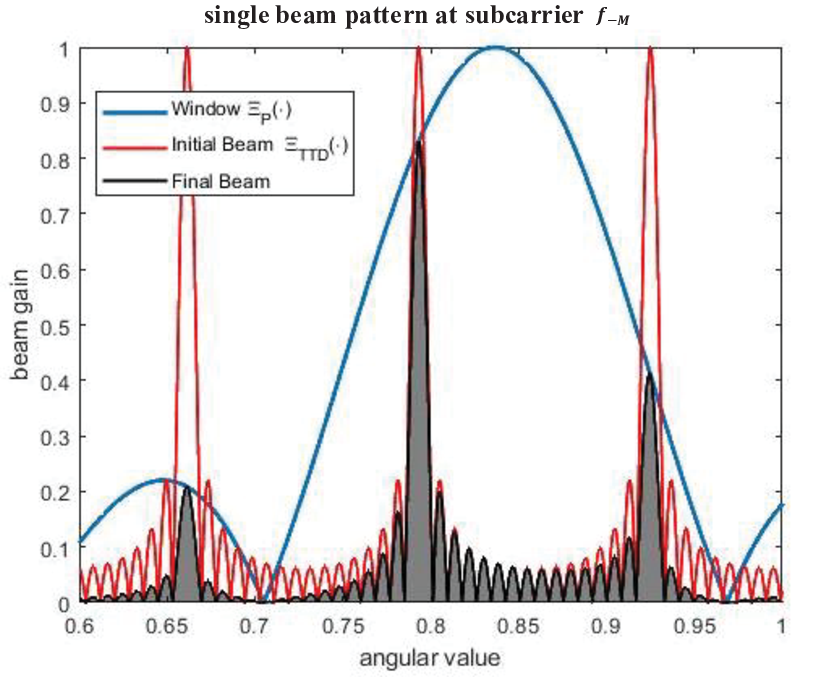
Based on the derivation in (12), we exploit some interesting properties of the two Dirichlet functions $\Xi_{P}(\cdot)$ and $\Xi_{N_{\text{TTD}}}(\cdot)$, which may be helpful for the following beam tracking and performance analysis. We herein regard real channel angle $\theta$ as the function argument. As for the former $\Xi_{P}(\frac{f_{m}}{f_{c}}\theta-\psi)$, the period, semi-width and the global-maximum point location are calculated as:

Similarly, as for the latter $\Xi_{N_{\text{TTD}}}(P(\frac{f_{m}}{f_{c}}\theta-\psi-\frac{f_{m}^{b}}{f_{c}}t))$, the period, semi-width and the global-maximum point location are

It is worth noting that the former period $T^{(1)}_{m}$ is much larger than $T^{(2)}_{m}$ and near to the width of argument interval $[-1,1]$. Therefore, we can regard the former Dirichlet function $\Xi_{P}(\frac{f_{m}}{f_{c}}\theta-\psi)$ as a window for the second term $\Xi_{N_{\text{TTD}}}(\cdot)$ and almost all components outside the main lobe of $\Xi_{P}$ are filtered to zero, as depicted in Fig. 2. Besides, notice that the former period $T^{(1)}_{m}$ is equal to the latter semi-width $W^{(2)}_{m}$, which means that there must exist only two peaks inside main lobe of $\Xi_{P}$ (when $\theta^{(1)}_{c,m}\neq\theta^{(2)}_{c,m}$). The maximum array gain at subcarrier $f_{m}$ almost always appears at $\theta=\theta_{m,c}^{(2)}+kT_{m}^{(2)}$ and must have $|\theta-\theta_{c,m}^{(1)}|<W_{m}^{(1)}$.

For wideband beamforming, we set PS and TTD parameters equal to the physical user direction $\theta_{0}$ ideally, i.e., $\psi=t=\theta_{0}$. In this way, the global-maximum point for array gain $\mathcal{G}$ locates at $\theta=\theta_{0}$ for all subcarriers $f_{m}$, which means beam squint is perfectly eliminated via TTD line.

As for TTD-aided wideband tracking, we configure the equivalent PS/TTD values $\psi,t$ bias to real beam angle. Notice the maximum array gain at subcarrier $f_{m}$ must lie in $\theta^{(2)}_{m,c}\ (+kT_{m}^{(2)})$ and thus we can strictly design the values of $\psi$ and $t$ to form particular beam patterns for tracking, i.e., establish a monotonical bijection between subcarriers $\{f_{m}\}$ and quantized angle set $\{\theta_{m}\}$ via maximum array gain location (15), i.e.,

where $\theta_{m}$ denotes the angular location with maximum beamforming gain at frequency $f_{m}$.

For clearer illustration of the frequency-scanning tracking, we provide the holistic gain distribution of overall subcarriers in Fig. 4(b), where $2M+1$ beamforming curves are plotted, corresponding to the whole $2M+1$ subcarriers. Each curve here displays a similar beam pattern to the gray region of Fig. 2. We can obviously observe the monotonical bijective relationship between subcarriers $\{f_{m}\}$ and quantized angular values $\{\theta_{m}\}$ in Fig. 4(b). Following this mechanism, we can easily screen the maximum beamforming gain, corresponding subcarrier and angular direction to implement tracking procedure in one timeslot.

In this section, we focus on the two tracking algorithms’ performance comparison and take the tracking range $\alpha$ as one important criterion, which directly controls the overhead consumption. Furthermore, one critical question is whether the range in (25) is maximum or not. Fortunately the answer is negative. An exquisite enlarged range with closed form is provided in this section ⁴⁴ 4 Without loss of generality, we only consider the spatial beam direction $\theta\in[0,1]$ and neglect the negative interval $[-1,0)$ in Section V and Section VI, due to its symmetry properties..

In this section, we give a joint consideration of TTD-aided tracking and beamforming. The above analysis is based on the infinite resolution of $\psi$ and $t$ in (11). However the beamforming codebook size is always countable in practice, which inspires us to evaluate the performance with finite beamforming codeword configuration.

As for beamforming module, given the DFT-based codeword pattern derived in (11), the quantization for $\psi$ and $t$ are easily yielded to

which denotes uniform quantization for the whole angular domain $[-1,1]$ with codebook size as $N_{\text{BS}}$ (resolution as $\Delta t^{\text{BF}}=2/N_{\text{BS}}$). Then at each subcarrier, $N_{\text{BS}}$ almost-orthogonal beams are generated to provide full communication direction coverage, just like the conventional narrowband DFT-based analog beamforming.

As for tracking module, in the forward-pairing scheme, substituting the radius constraint (20) to $t^{\text{fw}}$ (18), we can get that $t^{\text{fw}}=\frac{Mf_{d}}{f_{c}}\frac{1}{P}\geq 1$ since $\frac{1}{P}=\frac{N_{\text{TTD}}}{N_{\text{BS}}}\geq\frac{Mf_{d}}{f_{c}}$ according to [19, equ.25]. We can observe that the codewords in beamforming ($|t^{\text{BF}}|\leq 1$) and tracking ($t^{\text{fw}}>1$) are incompatible if we adopt the tracking radius upper bound (20), and thus the fixed radius $\alpha^{\text{fixed,fw}}$ should be further reduced from $\frac{1}{P}-\frac{Mf_{d}}{f_{c}}$. From another aspect, if we utilize the beamforming codebook (40) for forward-pairing track, we should ensure that $t^{\text{fw}}\leq 1$ and then get $\alpha^{\text{fw}}\leq\frac{Mf_{d}}{f_{c}}(1-\theta_{0})$, which means the fixed searching radius doesn’t exist at all.

References

- [1] H. Sarieddeen, N. Saeed, T. Y. Al-Naffouri, and M.-S. Alouini, “Next generation terahertz communications: A rendezvous of sensing, imaging, and localization,” IEEE Communications Magazine, vol. 58, no. 5, pp. 69–75, 2020.
- [2] Z. Chen, X. Ma, B. Zhang, Y. Zhang, Z. Niu, N. Kuang, W. Chen, L. Li, and S. Li, “A survey on terahertz communications,” China Communications, vol. 16, no. 2, pp. 1–35, 2019.
- [3] C. Lin, G. Y. Li, and L. Wang, “Subarray-based coordinated beamforming training for mmwave and sub-thz communications,” IEEE Journal on Selected Areas in Communications, vol. 35, no. 9, pp. 2115–2126, 2017.
- [4] H. Elayan, O. Amin, B. Shihada, R. M. Shubair, and M.-S. Alouini, “Terahertz band: The last piece of rf spectrum puzzle for communication systems,” IEEE Open Journal of the Communications Society, vol. 1, pp. 1–32, 2020.
- [5] K. Tekbıyık, A. R. Ekti, G. K. Kurt, and A. Görçin, “Terahertz band communication systems: Challenges, novelties and standardization efforts,” Physical Communication, vol. 35, p. 100700, 2019.
- [6] K. David and H. Berndt, “6g vision and requirements: Is there any need for beyond 5g?,” IEEE vehicular technology magazine, vol. 13, no. 3, pp. 72–80, 2018.
- [7] J. Hoydis, S. ten Brink, and M. Debbah, “Massive mimo in the ul/dl of cellular networks: How many antennas do we need?,” IEEE Journal on Selected Areas in Communications, vol. 31, no. 2, pp. 160–171, 2013.
- [8] T. L. Marzetta, “Noncooperative cellular wireless with unlimited numbers of base station antennas,” IEEE Transactions on Wireless Communications, vol. 9, no. 11, pp. 3590–3600, 2010.
- [9] O. E. Ayach, S. Rajagopal, S. Abu-Surra, Z. Pi, and R. W. Heath, “Spatially sparse precoding in millimeter wave mimo systems,” IEEE Transactions on Wireless Communications, vol. 13, no. 3, pp. 1499–1513, 2014.
- [10] X. Gao, L. Dai, S. Han, C.-L. I, and R. W. Heath, “Energy-efficient hybrid analog and digital precoding for mmwave mimo systems with large antenna arrays,” IEEE Journal on Selected Areas in Communications, vol. 34, no. 4, pp. 998–1009, 2016.
- [11] M. Wang, F. Gao, N. Shlezinger, M. F. Flanagan, and Y. C. Eldar, “A block sparsity based estimator for mmwave massive mimo channels with beam squint,” IEEE Transactions on Signal Processing, vol. 68, pp. 49–64, 2020.
- [12] B. Wang, M. Jian, F. Gao, G. Y. Li, and H. Lin, “Beam squint and channel estimation for wideband mmwave massive mimo-ofdm systems,” IEEE Transactions on Signal Processing, vol. 67, no. 23, pp. 5893–5908, 2019.
- [13] B. Wang, F. Gao, S. Jin, H. Lin, and G. Y. Li, “Spatial- and frequency-wideband effects in millimeter-wave massive mimo systems,” IEEE Transactions on Signal Processing, vol. 66, no. 13, pp. 3393–3406, 2018.
- [14] S. Targonski and D. Pozar, “Minimization of beam squint in microstrip reflectarrays using an offset feed,” in IEEE Antennas and Propagation Society International Symposium. 1996 Digest, vol. 2, pp. 1326–1329 vol.2, 1996.
- [15] B. Wang, X. Li, F. Gao, and G. Y. Li, “Power leakage elimination for wideband mmwave massive mimo-ofdm systems: An energy-focusing window approach,” IEEE Transactions on Signal Processing, vol. 67, no. 21, pp. 5479–5494, 2019.
- [16] F. Gao, B. Wang, C. Xing, J. An, and G. Y. Li, “Wideband beamforming for hybrid massive mimo terahertz communications,” IEEE Journal on Selected Areas in Communications, vol. 39, no. 6, pp. 1725–1740, 2021.
- [17] Q. Wan, J. Fang, Z. Chen, and H. Li, “Hybrid precoding and combining for millimeter wave/sub-thz mimo-ofdm systems with beam squint effects,” IEEE Transactions on Vehicular Technology, vol. 70, no. 8, pp. 8314–8319, 2021.
- [18] Y. Chen, Y. Xiong, D. Chen, T. Jiang, S. X. Ng, and L. Hanzo, “Hybrid precoding for wideband millimeter wave mimo systems in the face of beam squint,” IEEE Transactions on Wireless Communications, vol. 20, no. 3, pp. 1847–1860, 2021.
- [19] J. Tan and L. Dai, “Delay-phase precoding for thz massive mimo with beam split,” in 2019 IEEE Global Communications Conference (GLOBECOM), pp. 1–6, 2019.
- [20] K. Dovelos, M. Matthaiou, H. Q. Ngo, and B. Bellalta, “Channel estimation and hybrid combining for wideband terahertz massive mimo systems,” IEEE Journal on Selected Areas in Communications, vol. 39, no. 6, pp. 1604–1620, 2021.
- [21] E. Carrasco, J. A. Encinar, and M. Barba, “Bandwidth improvement in large reflectarrays by using true-time delay,” IEEE Transactions on Antennas and Propagation, vol. 56, no. 8, pp. 2496–2503, 2008.
- [22] E. Ghaderi, A. Sivadhasan Ramani, A. A. Rahimi, D. Heo, S. Shekhar, and S. Gupta, “An integrated discrete-time delay-compensating technique for large-array beamformers,” IEEE Transactions on Circuits and Systems I: Regular Papers, vol. 66, no. 9, pp. 3296–3306, 2019.
- [23] C. Qi, K. Chen, O. A. Dobre, and G. Y. Li, “Hierarchical codebook-based multiuser beam training for millimeter wave massive mimo,” IEEE Transactions on Wireless Communications, vol. 19, no. 12, pp. 8142–8152, 2020.
- [24] X. Gao, L. Dai, Y. Zhang, T. Xie, X. Dai, and Z. Wang, “Fast channel tracking for terahertz beamspace massive mimo systems,” IEEE Transactions on Vehicular Technology, vol. 66, no. 7, pp. 5689–5696, 2017.
- [25] J. Zhao, F. Gao, W. Jia, S. Zhang, S. Jin, and H. Lin, “Angle domain hybrid precoding and channel tracking for millimeter wave massive mimo systems,” IEEE Transactions on Wireless Communications, vol. 16, no. 10, pp. 6868–6880, 2017.
- [26] G. Arredondo, W. Chriss, and E. Walker, “A multipath fading simulator for mobile radio,” IEEE Transactions on Communications, vol. 21, no. 11, pp. 1325–1328, 1973.
- [27] J. Tan and L. Dai, “Wideband beam tracking in thz massive mimo systems,” IEEE Journal on Selected Areas in Communications, vol. 39, no. 6, pp. 1693–1710, 2021.
- [28] C. Han and Y. Chen, “Propagation modeling for wireless communications in the terahertz band,” IEEE Communications Magazine, vol. 56, no. 6, pp. 96–101, 2018.
- [29] R. J. Mailloux, Phased array antenna handbook. Artech house, 2017.
- [30] S. Boyd, S. P. Boyd, and L. Vandenberghe, Convex optimization. Cambridge university press, 2004.