Scalable multiscale-spectral GFEM with an application to composite aero-structuresJournal: Journal of Computational Physics
Abstract
In this paper, the first large-scale application of multiscale-spectral generalized finite element methods (MS-GFEM) to composite aero-structures is presented. The crucial novelty lies in the introduction of A-harmonicity in the local approximation spaces, which in contrast to [Babuska, Lipton, Multiscale Model. Simul. 9, 2011] is enforced more efficiently via a constraint in the local eigenproblems. This significant modification leads to excellent approximation properties, which turn out to be essential to capture accurately material strains and stresses with a low dimensional approximation space, hence maximising model order reduction. The implementation of the framework in the Distributed and Unified Numerics Environment (DUNE) software package, as well as a detailed description of all components of the method are presented and exemplified on a composite laminated beam under compressive loading. The excellent parallel scalability of the method, as well as its superior performance compared to the related, previously introduced GenEO method are demonstrated on two realistic application cases, including a C-shaped wing spar with complex geometry. Further, by allowing low-cost approximate solves for closely related models or geometries this efficient, novel technology provides the basis for future applications in optimisation or uncertainty quantification on challenging problems in composite aero-structures.
Keywords:
Multiscale-spectral Generalized Finite Element Methods (MS-GFEM) , GenEO coarse space , A-harmonic subspace , large-scale composite structure , parallel scalability1 Introduction
Ill-conditioned and multiscale partial differential equations (PDEs) arise in many fields, where the computation of a resolved, fine-scale solution or a robust low-dimensional approximation can be challenging. Due to the interaction of their mesoscopic structure (ply level; sub-millimeter scale) and their geometric macroscopic features (structural level; meter scale), composite aero-structures are naturally, inherently multiscale. To model the behavior of a large scale composite structure, the numerical model needs to accurately represent the meso-scale configuration of the material as well as the macro-scale geometry of the part. Full mesoscopic descriptions of large components naturally lead to models with huge numbers of degrees of freedom. This makes the computations prohibitively expensive, particularly in contexts where many evaluations are required, e.g. optimisation or uncertainty quantification. As a result, composite aero-structures provide an ideal test bed for the new multiscale method proposed in this paper, which allows for the interaction of fine and coarse scale behaviour to be captured without becoming excessive in cost.
1.1 High Performance Solvers for Composite Applications
Due to strongly varying parameters across the simulation domain, elasticity problems arising in composite materials lead to Finite Element (FE) matrices that are extremely ill-conditioned [1, 2]. This poor conditioning is due to the contrast in stiffness between the carbon fibres and the surrounding resin matrix, as well as the complex anisotropy arising from the inclusion of long directional fibres. As a result, composite laminates have both low-energy modes, whereby the stiff fibres act as rigid body inclusions and the complement resin deforms easily; and also very high-energy modes, in deformation regimes with stretched, stiff fibres. This contrast between low and high energy modes is at the heart of the ill-conditioning (high condition number) in composite applications.
Whilst sparse direct solvers, like UMFPACK [3] or the ones provided in the Abaqus package [4], can reliably solve such systems, they are inherently limited in their scalability. This immediately restricts the physical scale of composites that can be simulated. Iterative solvers such as Conjugate Gradient (CG) or GMRES [5] in turn promise massive parallel scalability for modern High Performance Computing (HPC) systems, but their efficiency (i.e. number of iterations) strongly depends on the condition number of the matrix.
In order to render such iterative solvers robust, preconditioners are essential. Whilst Algebraic Multigrid (AMG) preconditioners are in general a promising choice regarding robustness and scalability, tests with two AMG implementations, in dune-istl [6] and BoomerAMG [7], have demonstrated poor performance in composite applications [1, 2]. The reason is that, without a problem-specific local aggregation strategy, coarse grids in AMG do not capture the low-energy modes in composites structures, which motivates the search for alternative strategies that produce fast approximate coarse representations at a larger scale. The Generalized Eigenproblems in the Overlaps (GenEO) method [8] provides such a coarsening, leading to a robust, theoretical bound on the condition number of the preconditioned system for a two-level Schwarz Domain Decomposition (DD) method [9]. A problem-specific coarse space is computed from some tailored, local eigenproblems on overlapping subdomains. Robust scale-up to several thousands of processor cores for composites applications has been shown in [2, 10]. While the iterative solver now only needs few iterations, a considerable cost is expended in solving the independent local eigenproblems.
To avoid these tremendous computational costs of direct simulations of multiscale problems, computational homogenization methods [11, 12, 13] have been well developed and widely used in the engineering community. Moreover, in practical engineering applications, multiscale problems are typically solved multiple times with different source terms and possibly local changes in model parameters, such that the higher setup cost of such methods can be offset. Most of those methods, however, are based on scale separation hypotheses, and may fail for typical problems in realistic applications that do not exhibit such a scale separation.
1.2 Multiscale Methods in Composite Analysis
To efficiently solve multiscale problems without scale separation for repeated analysis required in an uncertainty quantification context, various multiscale model order reduction methods have been developed, such as the multiscale finite element method (MsFEM) [14], the generalized finite element method (GMsFEM) [15], localized orthogonal decomposition (LOD) [16], flux norm homogenization [17], and the generalized finite element method (GFEM) [18, 19, 20], to cite a few. Most of these methods were developed in the context of numerical multiscale methods and are based on representing the solution space on a coarse grid by a low dimensional space that is spanned by some pre-computed local basis functions that take into account the structural meso-scale information in the material parameters.
The multiscale-spectral generalized finite element method (MS-GFEM), the focus of this work, was first proposed by Babuska and Lipton [18] for solving heterogeneous diffusion problems, but motivated also by problems in linear elasticity and in particular fibre-reinforced composites. The approach builds optimal local approximation spaces from eigenvectors of local eigenproblems posed on A-harmonic spaces defined for oversampling subdomains. Crucially, the global approximation error is fully controlled by the local approximation errors, which are rigorously proved to decay nearly exponentially – a feature not shared by most other ad-hoc constructed numerical multiscale approaches. For diffusion problems the implementation details were discussed in [20] together with numerical results on a two-dimensional toy example.
In a recent paper [21], Ma, Scheichl and Dodwell proposed new local eigenproblems involving the partition of unity to construct new optimal local approximation spaces for the MS-GFEM method, resulting in a GenEO-type coarse-space approximation. Significant advantages of the new local approximation spaces were demonstrated and sharper decay rates for the local approximation errors were proved. In [22], the MS-GFEM method was then also formulated and analysed for the first time in the discrete setting, as a non-iterative domain decomposition type method for solving linear systems resulting from FE discretizations of the fine-scale problem. Very similar local and global error estimates as in the continuous setting were derived. Furthermore, an efficient method to solve the (discrete) local eigenproblems was proposed, where the A-harmonic condition is directly incorporated into the eigenproblem. More recently, this approach was applied to other multiscale PDEs, such as Helmholtz [23], parabolic [24] and singularly perturbed [25] problems. Although numerical results of various simple, two-dimensional examples have demonstrated the efficiency of the MS-GFEM method, up to now, there is no study available in the literature on the application of the MS-GFEM method to realistic, large-scale, three-dimensional multiscale problems and on the implementation and performance of the method on massively parallel computers.
1.3 Contributions of this paper
This paper represents the first large-scale application of GenEO as a multiscale-spectral GFEM, providing good approximations to fine-scale solutions with a very low number of basis functions. The reformulation of GenEO as a GFEM method in local A-harmonic subspaces distinguishes our methodology from the one proposed by Babuska and Lipton [19]. Most notably, in contrast to [19] our method is inherently adaptive — we can control the error a posteriori by simply setting a threshold on the eigenvalues to decide which eigenvectors need to be included into the local spaces; see Theorem 3.1. The paper constitutes an extension of the work proposed by Ma and co-authors [21, 22] by generalizing the method to three dimensional elasticity problems, demonstrated with two real-world application cases. The theoretical background of our formulation as well as its implementation are described in detail and its excellent performance and scalability are demonstrated. The resulting coarse space turns out to have significantly better approximation properties than GenEO in the elasticity problems considered here. In particular, local A-harmonicity is crucial for accurate strain approximation with significant practical improvements demonstrated in numerical experiments.
Our method provides efficient reduced order models for large-scale problems that exhibit strong dependence on local details. The efficiency arises from a decomposition of the global problem into independent sub-problems that can be treated fully in parallel. A scalability test is presented in this paper that demonstrates this high efficiency even for very large structures. The accuracy of the approximation space is fully adjustable: a single threshold parameter on the local eigenvalues allows for an optimisation of the amount of model order of reduction. The approach does not rely on a scale separation hypothesis between material scales (meso- and macro-scale for the examples illustrated in the paper), the proposed multi-scale framework is particularly well suited for composite aero-structures. This is demonstrated via an application on a realistic C-spar model – a demonstrator application in the UK-EPSRC-funded CerTest project on composite structural design and certification (see the acknowledgements in Section 7).
A key motivation for the approach presented in this paper is the development of an offline-online framework, where the costly local model order reductions are reused across multiple similar simulation runs, reducing the overall cost to a fraction, as suggested in [15] but with significantly smaller coarse spaces. This promises to accelerate uncertainty quantification or optimisation tasks on challenging composites models and will be described in detail in a subsequent paper.
In addition, this paper reports on other technical improvements and recent developments of the dune-composites module within DUNE [26]. Support for GenEO is extended to unstructured DUNE grids, which is crucial for engineering applications such as composite parts with complex geometry (e.g., T-joint stiffeners) that cannot be discretized solely using a structured grid. Since the implementations of unstructured grids do not natively support overlapping subdomains in DUNE, the overlapping FE matrices needed in GenEO are constructed directly from assembled ones on a non-overlapping grid partition.
2 Problem formulation
Let us start by formulating the anisotropic, linear elasticity equations for composite structures and their finite element discretization. The composite structure is assumed to occupy a bounded and (for simplicity) polyhedral domain with boundary and unit, outward normal . At each point we define a vector-valued displacement and denote by the body force per unit volume. The infinitesimal strain tensor, is defined as the symmetric part of the displacement gradients:
| (1) |
where . The strain tensor is connected to the Cauchy stress tensor via the generalized Hooke’s law:
| (2) |
where the material tensor is a symmetric, positive definite fourth order tensor. The studied material will be further described in Section 5.1.
Now, let and be disjoint open subsets of such that and consider the function space
| (3) |
Given functions and , prescribing the Dirichlet and Neumann boundary data, the weak formulation of the problem to be considered consists in seeking the unknown displacement field with on such that
| (4) |
where the bilinear form and the functional are defined by
| (5) |
The variational problem (4) is discretized with conforming FEs on a mesh on by introducing the FE space as the tensor product of the spaces , spanned by the usual Lagrange bases on . We find a function such that on and then seek an approximation , where , such that
| (6) |
We block together displacements from all three space dimensions, so that denotes the vector of displacement coefficients containing all space components associated with the basis function. The displacement vector at a point is then given by , . The system (6) is equivalent to a symmetric positive-definite (spd) system of algebraic equations:
| (7) |
The blocks in the global stiffness matrix and in the load vector, for any , are given by and . The vector is the block vector of unknown FE coefficients.
System (7) can be assembled elementwise using Gaussian integration:
| (8) |
The elementwise bilinear form is trivial to obtain here by restricting the integrals in eq. 4 to . Later, restrictions of to mesh-resolved subdomains will be crucial in defining coarse space approximations. For any mesh-resolved subdomain , the restriction of to is denoted by
| (9) |
3 Multiscale-spectral generalized finite element method
In this section, the methods employed in this paper are defined alongside some theoretical results. In addition to generalized finite element methods (GFEM), we also describe the GenEO space, which was originally designed as a coarse space for two-level additive Schwarz methods in [8]. Here, it is for the first time applied as a multiscale method for stand-alone coarse approximation to a realistic three-dimensional multiscale problem in composites, in the form of the multiscale-spectral generalized finite element method (MS-GFEM) method [18, 21, 22].
3.1 Domain decomposition

Both the two-level additive Schwarz method and GFEM are based on a decomposition of the domain into non-overlapping subdomains that are resolved by the mesh ; see Figure 1 for an example. Each non-overlapping subdomain is extended by adding layers of neighboring elements to create an overlapping partition of .
Next, the local finite element (FE) spaces
are defined, where the former restricts to the subdomain while the latter restricts this space further to functions whose support is contained entirely in .
A key ingredient of GenEO-type coarse spaces and of GFEM is a partition of unity (PoU) subordinate to the overlapping decomposition . A particular partition of unity specific to the FE setting was constructed in [8]. For each , let
| (10) |
denote the set of internal degrees of freedom in , and define for each degree of freedom a weight such that
With these weights we can define a family of local partition of unity operators , , such that
| (11) |
It follows immediately from the definition that the operators satisfy
| (12) |
Here denotes the prolongation operator defined as the extension of a function in by zero. In [8], it was suggested that the weights can be set as
that is, one over the number of subdomains that contain as an internal degree of Freedom (DoF). Other partitions of unity can also be used. In the numerical experiments below, we will use a different (smoother) partition of unity.
3.2 GenEO coarse space
The GenEO space – designed in the context of additive Schwarz preconditioning methods, as a robust coarse space correction for multiscale variational problems – is based on the following generalized eigenvalue problem (GEVP) on each subdomain : Find , such that
| (13) |
In the original publication [8], the bilinear form on the right hand side of (13) was restricted to the overlap , but as shown in subsequent publications, such as [27], the GenEO space defined by the GEVP in (13) has very similar coarse space correction properties.
Only the lowest-energy eigenfunctions in (13), i.e., the ones corresponding to the smallest eigenvalues, are used to define the GenEO coarse space. Denote by and the -th smallest eigenvalue and the corresponding eigenfunction on subdomain . Then, the GenEO coarse space is defined by
| (14) |
where the partition of unity operators are used to "stitch" the local approximation spaces on the subdomains together and to guarantee that . This definition of still leaves open the number of eigenfunctions to be included.
In the context of two-level additive Schwarz methods, where the GenEO coarse space is combined (additively) with local solves on the overlapping subdomains to obtain a preconditioning matrix for , it is then possible to bound the condition number of the preconditioned system independently of the mesh size , the subdomain size or the heterogeneity in the coefficient. In particular, [8, Corollary 3.23] states
| (15) |
where is a typically small constant depending only on , the maximum number of subdomains overlapping at any point. Thus, the condition number can be controlled by choosing the number of eigenfunctions per subdomain such that is bounded uniformly across all subdomains. The eigenvalues converge to as increases, but no theoretical results on the rate of convergence exist in general.
3.3 Generalized FE methods with GenEO-type local approximation
The GenEO space in (14) is in essence a global approximation space of generalized FEM type [28], where a fairly arbitrary family of local approximation spaces can be "stitched" together via a partition of unity to build the global space. As such, for (the subdomain size) sufficiently small or for sufficiently large, it is possible to solve the FE problem directly to a required accuracy in , in the spirit of the GFEM. However, as we will see below in the numerical experiments, the rate of convergence with respect to is rather poor when the local bases are computed as in (13). A significantly more efficient GFEM can be designed by slightly modifying the GEVP (13) as shown in the following.
In this subsection, a particular family of GenEO-type local approximation spaces is constructed and used within the framework of the GFEM as a stand-alone coarse approximation. Compared with the original version, there are two key ingredients in this GenEO-type coarse space that provide a better accuracy for coarse approximation. The first is oversampling. Similarly to the construction of the overlapping subdomains, we extend each overlapping subdomain further by adding more layers of fine-mesh elements to create an oversampling subdomain . The local eigenproblems used for constructing the coarse space will be defined on instead of . The second ingredient is A-harmonicity. To make this notion precise, we first introduce the following local FE spaces defined on the oversampling domains:
| (16) |
| (17) |
The space consists of FE functions restricted to that vanish on the external Dirichlet boundary of , whereas consists of FE functions that vanish on both the external Dirichlet boundary and the interior boundary of . The A-harmonic local FE space on is then defined as
| (18) |
Functions in are referred to as A-harmonic FE functions. As we will see below, the local eigenvectors used for building the coarse space are A-harmonic FE functions instead of general FE functions.
With the above notations, we now define a local eigenproblem similar to (13) on each oversampling subdomain: Find , such that
| (19) |
Note that since and can be identified with FE functions in , the right-hand side of the above GEVP is well-defined.
Let denote the -th eigenpair of the GEVP (19) with eigenvalues enumerated in increasing order. The desired GenEO-type GFEM coarse space is defined almost identically to the standard version (14):
| (20) |
The last ingredient of the MS-GFEM method is a global particular function built from local particular functions. On each oversampling subdomain , we first define a local particular function , where satisfies
| (21) |
with being the restriction of to , and satisfies on and
| (22) |
Note that vanishes on all interior subdomains where or whenever on . On subdomains intersecting it would in fact be possible to combine problems (21) and (22) into one local problem, but this leads to a slightly larger constant in Theorem 3.1 below. Therefore, we work with local particular functions defined via (21) and (22) in this paper. The global particular function is then defined by “stitching” together the local functions using the partition of unity:
| (23) |
Having defined the coarse space and the global particular function , we are now ready to give the MS-GFEM method for solving the fine-scale FE problem (6): Find , where , such that
| (24) |
To assess the quality of the MS-GFEM approximation, we estimate the energy norm of the error . Following the lines of the proofs of Theorems 2.1 and 3.4 in [21], we can derive the following bound:
Theorem 3.1.
| (25) |
is known explicitly and bounded by the maximum number of oversampling domains that overlap at any given point in , and is the smallest eigenvalue corresponding to any eigenvector not included in the local basis on .
Thus, the efficiency of the MS-GFEM method is controlled by the speed at which the eigenvalues in (19) grow. To estimate this growth rate, let and denote the diameter of and , respectively. The following (informal) theorem in dimensions, similar to Theorem 4.6 in [22], gives an exponential bound on the eigenvalues, which can be proved following the lines of the proofs of Theorem 4.6 in [22] and Theorem 7.3 in [19] (details will be given in a forthcoming paper).
Theorem 3.2.
Let be sufficiently small. Then there exist independent of , such that for
| (26) |
The constants , and can again be derived explicitly. The value of and thus the convergence rate grows with the amount of oversampling, i.e., with decreasing .
Combining the exponential bound (26) on the local eigenvalues and the global error estimate (25) provides a rigorous, exponential error bound for the MS-GFEM method. It is important to note that the exponential growth rate of the local eigenvalues critically relies on the two aforementioned ingredients of the new coarse space, i.e., oversampling and A-harmonicity. The global error estimate (25) also holds for the standard GenEO coarse space when used as a coarse approximation. However, without the two key ingredients, the eigenvalues of the local GEVP (13) do not grow exponentially fast, making the standard GenEO coarse space significantly less efficient; see Subsection 5.4.
Apart from the exponential decay rate of the error with respect to the number of local basis functions, Theorem 3.2 also provides an explicit decay rate of the error with respect to the oversampling size, which offers a second handle to control the error of the method, in addition to a change in the size of the local approximation spaces. This turns out to be of great importance in reducing the size of the global coarse problem; see Subsection 5.6.
We end this subsection by discussing ways to solve the local GEVP (19). Due to the presence of the A-harmonic condition, a straightforward yet time-consuming way of solving (19) is to first construct the basis functions of the A-harmonic FE space by solving many local boundary value problems [18, 20, 29]. Instead, we use a different and more efficient method proposed in [22], where the A-harmonic condition is directly incorporated into the local GEVP. To this end, a Lagrange multiplier is introduced and the local GEVP (19) is rewritten in an equivalent mixed formulation: Find , and such that
| (27) | ||||||
The implementation details of how the augmented system (27) is solved are presented in Subsection 4.3.
4 Implementation
The DUNE [26] package is an open-source, modular toolbox for the numerical solution of PDE problems. It leverages advanced C++ programming techniques in order to provide modularity from the ground up while producing highly efficient applications. As such, it allows the reuse of many existing components when implementing our new mathematical methods for HPC applications. The new methods were integrated in the dune-composites module [1], which facilitates setting up elasticity models and provides access to efficient solvers that scale to thousands of cores on modern HPC systems, despite the typically bad conditioning of composites problems. This was achieved through an HPC-scale GenEO implementation [10] developed as part of dune-composites and later moved into the lower-level discretization module dune-pdelab [30] within DUNE. The dune-pdelab module and several lower-level DUNE modules are used within dune-composites to obtain the finite element discretizations on the fine level.
Within the DUNE framework a number of grid implementations are provided for various purposes. Initially, only YASPGrid, a structured grid, provided native support for overlapping domain decomposition methods, where each process holds a copy of elements in its overlap region and may exchange data attached to associated DoF s with neighboring processes. Since the methods considered here are constructed using overlapping subdomains, we need this kind of communication mechanism. In previous work within dune-composites [1], the restriction to cuboid domains induced by YASPGrid was overcome by applying a geometric transformation to the grid. However, for many relevant engineering applications, a smooth transformation from a cuboid geometry to the actual geometry is not available. Thus, DoF-based communication was extended to support unstructured grids as well. In order to handle more general model geometries, the grid creation was first shifted to a pre-processing step using Gmsh [31]. The grid import is facilitated by the IO functionality of dune-grid.
4.1 Algebraic overlap construction for GenEO
In order to provide overlap and communication across overlaps on unstructured grids, an algebraic approach was introduced where finite element matrices defined on overlapping subdomains are constructed from corresponding matrices assembled on non-overlapping subdomains .
Figure 1 illustrates our notation for non-overlapping and overlapping subdomains. We begin with a matrix on a non-overlapping subdomain , and assume it has neighboring subdomains , , with corresponding matrices . We identify coinciding DoF s in and through a global indexing, as provided by non-overlapping DUNE grids. On subdomain , we now identify all DoF s directly connected to those in , and provide process with unique indices and the connectivity graph of this newly identified layer of DoF s. Since connected DoF s in a FE discretization are either associated with the same element or adjacent elements, we now are in a position where each process is aware of its neighbors’ DoF s within the first layer of elements along the respective boundary.
By a recursive application of this algorithm, as shown in Figure 2, we can now grow the algebraic overlap by an arbitrary number of layers of elements, without having to rely on the grid implementation to provide connectivity graphs. In the following, we will define the number of layers of elements added to a subdomain as (for overlap) – even though the overlap of a domain with its neighbour is in fact . Finally, using the extended connectivity graphs above we can construct a communication mechanism between neighbors to exchange overlap data of vectors defined on the extended domains. We now have the communication infrastructure to generate a GenEO space in a parallel way in place . While the method above allows us to extend connectivity graphs of non-overlapping matrices into neighboring subdomains, mimicking the connectivity graphs of the overlapping matrices , the GenEO method obviously requires the actual matrix entries. Using communication across the algebraic overlap, the required matrix entries can be exchanged between neighbors. This relies on the basic assumption (satisfied in general) that the bilinear form of the weak formulation can be decomposed additively into elementwise bilinear forms , such that with the grid on . For linear elasticity this is trivially satisfied, see (8).
As a result, retrieving matrix entries from neighbors and adding them where DoF s belong to multiple subdomains leads to a correct construction of an overlapping subdomain matrix from non-overlapping ones. There is one exception however: At the boundary of the overlapping domain, retrieving the entries of an interior DoF will not yield the correct result since the integration domain of said interior DoF extends beyond as shown in Figure 3. We circumvent this issue by not sending individual matrix entries in from process to process , but instead by assembling a new matrix on the domain for that purpose as shown in Figure 4. In practice, we communicate the partition of unity generated from the already available matrix graph of to all neighbors, and use as a convenient proxy to the desired domain snippet. Since we have the decomposition
all snippets together form the desired overlapping subdomain. Exploiting additivity of the bilinear form and of the FE matrix entries, this assembly strategy delivers the correct overlapping matrix for .
4.2 Partition of Unity and oversampling
As explained in section 3.1, various partition of unity operators can be used in the GenEO theory, as long as they fulfill condition (11). One suitable choice is a smooth transition from zero on to one on , as illustrated in Figure 5 (left). It is the choice made for the GenEO coarse space in [1] (where it is used as a preconditioner). To construct this partition of unity, a weight is attributed to each DoF . Initially, is set to on and to on the remaining vertices in , where is the number of layers added. For each DoF , using the extended connectivity graph of in its vicinity and comparing with neighboring weights, the weight is then reduced incrementally in the subdomain interior such that
where are the neighboring DoF s of . It suffices to iterate this times. As an example, the partition of unity in Figure 5 (left) has been constructed with . The communication mechanism between subdomains is used to associate to each DoF their corresponding counterpart in the neighboring subdomain . The partition of unity is then simply defined as:
where is the number of subdomains sharing the DoF .
The handling of oversampling subdomains is controlled via the choice of the partition of unity. The implementation of the partition of unity for the oversampled subdomains is the same as the one described above with a different initialisation of . In particular, is initialized to not only on , but also for a further layers of DoF s before applying the iterative process above. Thus, the partition of unity is a vector defined on the full oversampling subdomain that takes the value zero on . In the following, we will choose a variable oversampling size and keep one layer of non-zero partition of unity overlap, i.e., , as shown in Figure 5 (right).

4.3 Enforcing A-harmonicity within the GEVP in DUNE
As described in [22], the eq. 27 can be formulated as a matrix eigenvalue problem. To achieve that, the DoF associate with are partition into three sets:
Those sets of DoF are depicted in Figure 1. We also define as the sizes of the corresponding set . The GEVP in matrix form is defined as follows: Find , and :
| (28) |
where and . The blocks , , are zero since the partition of unity vanishes on . The oversampling, created via the choice of partition of unity, will also affect the the right hand side of eq. 28, such that not only the blocks , , but also all entries in corresponding to the oversampling region will be zero (see Figure 5). The GEVP solution to construct the local basis is then , where is a zero-vector corresponding to the DoF s in , which combined with provides an A-harmonic coefficient vector on all of . Instead of generating each block individually, it is extracted from using the sets of DoF s . In practice, the matrix
is built by block. The top left block is obtained by removing the rows and columns corresponding to from . In the elasticity case, Dirichlet boundary conditions are imposed in DUNE by altering rows in the matrix – one on the diagonal, zero elsewhere – so the set can be easily detected. Then finally is obtained by removing the rows and columns corresponding to . The block that is removed corresponds to . DoF s belonging to are detected and saved during the overlap creation phase.
Once the basis is obtained, the next step in the construction of the coarse space is to multiply the eigenvectors by the partition of unity, see eq. 14. To improve the conditioning of the coarse space problem, a re-orthogonalization step via a Gram-Schmidt process is carried out following this multiplication. Contrary to [22], we have implemented directly eq. 28, since the simplification of eq. 28 proposed in [22] for diffusion problems requires a special handling of subdomains that are only affected by Neumann boundaries , which is more involved for linear elasticity in 3D.
4.4 Boundary conditions at the coarse level
The eigenvectors of the local GEVP s have to be combined with local particular solutions if the body force is nonzero or if touches the global Dirichlet boundary and the boundary displacement is nonzero. A particular solution is obtained by solving the local partial differential equation (PDE)
The solution is then multiplied by the partition of unity and orthogonalized with respect to using again Gram-Schmidt. We denote the resulting vector by . This vector is then normalized and appended to the basis.
At the coarse level, inhomogeneous Dirichlet boundary conditions are imposed by altering the coarse matrix and the coarse vector . If denotes the index of the particular solution on subdomain in the coarse system, then a Dirichlet boundary condition, imposed on via the particular solution , is enforced in the coarse system by setting:
4.5 Hardware and software
For solving the local GEVP, we use Arpack [32] through the Arpack++ wrapper in symmetric shift-invert mode. As subdomain solver, we use UMFPack [3] in the eigenvalue solver. The domain partition of into non-overlapping subdomains is carried out by the graph partitioner ParMetis [33].
The numerical results have been carried out on the Hamilton HPC Service at Durham University. Its last version, called Hamilton8, provides a total of 15,616 CPU cores, 36TB RAM and 1.9PB disk space. Hamilton8 is composed of 120 standard compute nodes, each with 128 CPU cores (2x AMD EPYC 7702), 256GB RAM and 400GB local SSD storage.
5 Numerical Experiments: Performance tests for MS-GFEM on composite structures
Throughout this paper, we assume a linear elastic behavior of the composite material. For aerospace applications, considering damage behavior is essential. Ultimately, our framework will be applied to model large displacement effects and the onset of failure. To achieve this, two requirements need to be validated. Firstly, it is essential to have an efficient linear elastic solver for a large-scale model to be used within any non-linear iteration. Secondly, the approximate solution needs to accurately represent relevant damage criteria, especially local extrema.
In this section, after a brief description of the composite models, we first analyse the output from all components of the MS-GFEM when applied to a composite beam. The method is then applied to a complex, aerospace part using a composite failure criterion to assess the accuracy. Finally, the parallel scaling of the method is investigated, demonstrating the efficiency of the proposed MS-GFEM on large composite structures.
5.1 Specification of the considered composite model problems

In the following three subsections, first a laminated beam under compression is considered in order to evaluate the performance of the method proposed in this study. It is illustrated in Figure 6 (a). The laminated beam has a length of mm, a width of mm and a thickness of mm. The laminate is made up of a stack of three layers (or plies) of the same thickness. Each layer represents a uni-directional composite made up of carbon fibres embedded into resin. Plies are modelled as homogeneous orthotropic elastic materials, characterised by nine parameters and a vector of orientations . The elastic properties of AS4/8552 ([34]) have been chosen for this example. In the global coordinate system, the material tensor is orientated using standard tensor rotations, following the stacking sequence []. For more details see, e.g., [35]. The study considers the elastic behavior of the laminated beam under compression. The uni-axial compression, illustrated in Figure 7(b), is modeled as a displacement imposed Dirichlet boundary condition.
Then for the remainder of the paper, a realistic aerospace part is used to demonstrate the high quality of the achieved coarse approximation. The aerospace part in question is a mm long C-shaped wing spar section (C-spar) with a joggle region in its center, creating a geometric feature in the structure, see Figure 6 (b). The material is a laminated composite, composed of 24 uni-directional layers (carbon fibers and resin) of each, which are orientated as follows:
The behavior of the C-spar under compression will be investigated using the same boundary conditions as the ones used in the beam example above.
In both examples, as visualized in Figure 6, for the local approximation we use FE grids with piecewise linear elements, reduced integration to avoid shear-locking and one element through thickness per layer.
5.2 Local GEVP outputs

We start by analysing the local generalized eigenvalue problems (GEVP), in particular the behavior of the smallest eigenvalue corresponding to any eigenvector not included in the local approximation space, which is the main parameter driving the method accuracy (cf. the error bound in eq. 25). First, the decay of for representative subdomains is analysed, as well as the shape of the associated eigenvectors. Then, the effect of the oversampling size is discussed. A particular focus will be on the local finite element aspect ratio which severely affects the accuracy of the computed eigenvectors/-values and thus also the observed actual decay of the error bound.
The beam domain in Figure 6 (a) is decomposed into subdomains for the first experiment; see Fig. 7 (b). In each subdomain, a local eigenvalue problem is solved to construct the local approximation space with a fixed number of oversampling layers. In Figure 7 (c,d) a selection of exemplary, local GEVP solutions on two representative subdomains are presented together with a semi-logarithmic plot of in Fig. 7(a). For the eigenvalue plot two further subdomains are added. In total, there is one subdomain intersecting (), one intersecting and two interior subdomains (), with the first one of the two having a higher surface-to-volume ratio.
The semi-logarithmic plot of in Fig. 7(a) demonstrates the predicted, nearly exponential decay of the local approximation error with respect to the basis size () in all cases. The decay is faster for subdomains intersecting ; the more the subdomain intersects the faster is the decay. A further factor is the surface-to-volume ratio. The higher this ratio the slower the exponential decay of , as exemplified by the relative decays of subdomains and . The partitioning of the domain could be optimised to unify the surface-to-volume ratio over all subdomains. In fact, for simple, laminated composites a regular domain decomposition could be chosen, e.g., into rectangular subdomains. Here, however, we do not make this choice in order to show the robustness of the approach to rather general subdomain partitionings, as provided by automatic graph partitioners such as ParMetis [33], and thus to show the potential of the approach for simulating very complex structures.
In the interior subdomain , the first six eigenvectors (indices to ) depicted in Figure 7 (d) correspond to the zero energy modes (or rigid body modes) representing shifts and rotations of the structure. The following modes for and the first few modes for in Figure 7 (c) correspond to low-energy deformations of the subdomain: bending and shearing. The higher-energy modes correspond to higher frequency deformations ().

As explained in Section 3.3, the oversampling parameter is key to the decay rate of the local approximation errors. In Figure 8, the reciprocal eigenvalues for subdomain are presented for a range of oversampling sizes. The decay of clearly accelerates as the oversampling size is increased. Thus, for a desired error bound (i.e. ), subdomains with larger amounts of oversampling lead to significantly smaller local bases and consequently to an overall smaller coarse space. The trade-off, however, is that the dimensions of the local GEVP s grow significantly with the amount of oversampling and this will be discussed later. In general, the objective is to pick the minimal number of modes to approximate the solution (displacement) and its derivative (strain and stress) sufficiently well. The accuracy of the coarse approximation and the effect of changing the main tuning parameters (basis / oversampling size) will be analysed in Section 5.3. The efficiency study will be performed for the more complex C-spar structure and is presented in Section 5.6.

The results in Figures 7 and 8 are computed using square elements with an aspect ratio of one between horizontal (through-thickness) and vertical (in-plane) edges. However, such a choice leads to an unreasonably high number of elements in larger composite structures with a larger number of more realistic, thinner plies, such as the C-spar described in Section 5.1 and depicted at he bottom of Figure 6. To build a reasonably sized model, the in-plane discretization has to be reduced, leading to flat elements with a larger aspect ratio. Unfortunately this reduces the accuracy significantly, as presented for four element aspect ratios and in Figure 9 (b), where the relative -error for each eigenpair is shown. As a consequence, after a similar initial decay (up to ) we observe a change in the slope of for aspect ratios bigger than one in Figure 9 (a). For very large aspect ratios of 15 and above, it even leads to a plateau in (see Figure 7 (a), red curve). This is to be expected, due to the larger condition numbers of the stiffness matrices in the GEVP leading to more unstable eigensolves.
Increasing the oversampling size does not alleviate this problem, as seen in Figure 9 (c,d); the relative -errors in the eigenpairs are independent of and the slope of changes roughly at the same value of . We also tested a different type of higher-order finite element, namely a 20-DoF quadratic serendipity element, but the loss of accuracy due to high element aspect ratios persists. However, the slope change and the plateau of the eigenvalues for larger aspect ratios do not have a strong impact, since they occur only at values well below what is needed for good practial approximation, especially for higher oversampling sizes.
5.3 Coarse approximation accuracy
In this section, we investigate the accuracy of the MS-GFEM approximation. The fine-scale reference solution is computed using an iterative CG method with GenEO as preconditioner. By setting a sufficiently low tolerance, the error due to the iterative solution via CG can be neglected.
We consider in the following the relative errors in -norm between the coarse approximations of displacement and strain fields, and , and their fine-scale counterparts, and , i.e.,
Figure 10 (a) shows the fine-scale approximation of the displacement field of the beam under compressive loading. The unit displacement ( mm) applied here causes the characteristic out-of-plane deformation of the structure related to the non-symmetric stacking sequence chosen for this example. A maximum displacement of mm is observed on the two sides of the beam. Figure 10 (b) depicts the fine-scale strain approximation in the direction of compression, denoted by here. The order of magnitude of strains is .

The main parameter driving the accuracy of the coarse approximation is the smallest eigenvalue corresponding to any local eigenvector not included in the basis. As explained above, the size of each of the local bases and the oversampling size will be decisive to control this parameter. For our analysis we vary these two key parameters up to maxima of and , for which the error bound lies below . The relative -errors for displacement and strain are shown in Figure 10, resp. (c) and (d), using a logarithmic scale. Both and decay exponentially with respect to for all amounts of oversampling. The decay rate of the errors is higher for larger oversampling sizes, which is in agreement with the behavior of the reciprocal eigenvalues depicted in Figure 8.
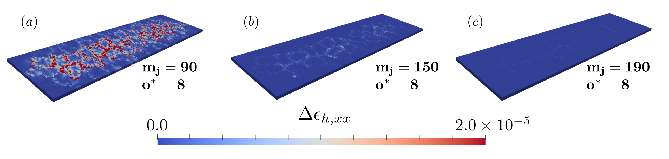
We further investigate the location of the largest strain error, in order to explain in more detail its dependence on and . The coarse approximation of the strain field has been projected onto the fine-scale space to allow a direct comparison element-by-element. The absolute differences between the fine-scale solution and the coarse approximation of the strain field are depicted in Figure 11 for three different values of the local basis size per subdomain, , and a fixed value of . The aim is to investigate the error behavior alongside the convergence curve for in Figure 10 (d). The three chosen basis sizes produce coarse-space solutions of high accuracy with relative -errors bellow . The error maxima are observed on subdomains located in the center of the beam. Indeed, the local error on each subdomain follows the decrease of . As shown in Figure 7 (a), interior subdomains (e.g., ) need more eigenvectors for the same local error. Eventually, a sufficiently large local basis size ensures an accurate approximation for all subdomains.

Conversely, for fixed Figure 12 assesses the impact of the oversampling size, varying . As expected, small oversampling size leads to an error localised at subdomain interfaces. Increasing the oversampling area decreases the interface errors, and, eventually a smooth and very low error is observed across the domain for . This example showcases one of the main advantages of the MS-GFEM: the interface problem at subdomain boundaries is handled by oversampling. Thus, the approximation is then robust to the chosen domain decomposition and there is no scale separation between the ply scale (mesoscopic) and the structural scale (macroscopic).

In Figure 13, the strain error is evaluated for a fixed eigenvalue threshold for various oversampling sizes, to study the impact on the overall coarse space size. For fixed accuracy, the size of the coarse space is reduced by when increasing to and by from to . This improved model order reduction obviously reduces the cost of the coarse problem solve, but it does increase the size of the local problems and thus the cost of solving the local GEVPs. This cost trade-off will be studied more carefully in Section 5.6 for the C-spar.
5.4 Importance of the A-harmonic condition for composite problems

To emphasize the necessity of the A-harmonic condition in our framework, we compare the new MS-GFEM space to the classic GenEO coarse space with the GEVPs formulated directly in the FE space , i.e., without enforcing A-harmonicity. The theoretical error bound in Theorem 3.1 is the same for both GFEM spaces, with and without the A-harmonic condition in the GEVP. Crucially, in both cases the approximation error is bounded by the reciprocal of the smallest eigenvalue corresponding to any eigenvector that is not included in the coarse space .
Figure 14 (right) shows that the decay of for is comparable between classic GenEO and the A-harmonic formulation, since the first modes (rigid body, shear and bending) appear in both. In fact, the classic GenEO coarse space with a small number of lowest-eigenvalue modes was shown in Reinarz et al. [2] to provide a robust preconditioner within CG that reduces the condition number effectively and leads to a low number of CG iterations for composites problems. Beyond that, we observe in Figure 14 (right) that the spectrum for the classic GenEO formulation decays much slower and eventually almost stagnates, when compared to MS-GFEM. This is reflected in the coarse approximation error in Figure 14 (left), as predicted in Theorem 3.1.Even including eigenvectors in classic GenEO is not sufficient to accurately represent the strain field in this application (with ). MS-GFEM with A-harmonic GEVPs, on the other hand, achieves an excellent coarse approximation at much lower basis sizes.
5.5 Method accuracy on an aerospace part

In this section, the behavior of the C-spar, described in Section 5.1, under compression is investigated. The domain, shown in Figure 6 (b), is divided into subdomains. For an oversampling size of and a tolerance of on we obtain local basis sizes varying between and . These parameters lead to an average subdomain size of and a model order reduction of . With 4GB of RAM per subdomain to compute the local GEVP this parameter choice requires 4 nodes of the HPC cluster Hamilton8 for the 256 subdomains. The element aspect ratio is 15 for this example (see Figure 6). Thus, as for the simple beam example, the possible coarse approximation accuracy is limited by the fine scale error.
In order to assess the coarse approximation, the longitudinal compressive failure criterion
| (29) |
from [36] is computed, which is a linear combination of relevant stress components: transverse and shear. A detailed description of the material parameters that are involved is outlined in [36]; the notation denotes the positive part of the argument. It represents the initiation of the fiber kinking mechanism, observed for fiber reinforced composites under compression. In slender composite structures, this failure mode typically appears after the buckling of the structure, but even in the pre-buckling context, this criterion gives a good insight into the usefulness of the method for studying compressive failure.
The elementwise longitudinal compressive failure criterion, computed in local coordinates, is plotted in Figure 15 (a). To compute it the coarse approximation is first projected onto the fine scale FE space . The relative error with respect to a direct meso-scale approximation in is shown in Figure 15 (b). With the chosen parameters, the relative error on the failure criterion is below . In Figure 15 (a), four plies (ply 6, 12, 18 and 24) are highlighted in a certain part of the domain, representing each stacking orientation and showing that the coarse approximation is able to accurately represent the quick variation of the compressive failure criterion through thickness. The remaining error is small and uniformly distributed, with higher values near subdomain boundaries and on interior subdomains, in agreement with the observations on the beam example.
5.6 Method scalability

A parallel (weak) scaling test of the method is presented in Figure 16, where the cost of the local GEVP solves and the cost of the coarse solve are assessed using C-spars of different lengths while fixing the discretization of the meso-structure: elements through thickness (one per ply) and a constant element size in the other directions (aspect ratio 15). The C-spar models vary between mm with (Model 1) and m with (Model 7). The number of processors () employed for each model have been chosen such that remains constant.
Three combinations of parameters have been tested, choosing and and selecting a threshold of and for the reciprocal of the local eigenvalues. Parameter sets and assess the scalability of the method for a highly accurate solution with . In Set , chosen to reduce RAM consumption, whereas in Set a larger oversampling size of is selected, thus requiring more RAM. This trade-off will be further discussed below. Set has been selected to study how the method scales for a lower eigenvalue threshold of with smaller and half the amount of subdomains in Sets and , such that is roughly the same.
For all three sets, the GEVP solve step scales perfectly, since it requires no parallel communication. As expected the local GEVP solve times increase slightly between Sets and due to the slightly bigger local problem sizes. The overall cost for the coarse space setup for each model is essentially identical, since it is dominated by the cost of solving the local GEVPs and can also be carried out fully in parallel with only some local data exchange. In contrast, the final coarse space problem (24) is (currently) solved on one processor, and thus eventually dominates the overall cost for larger models. To remain efficient, the coarse space size needs to be optimized. For all considered models, the model order reduction is around for Set and around for Set . As a consequence, the increase in oversampling size from Set to Set significantly reduces the cost of the coarse solve, particularly for the larger models (4–5–6). These gains clearly outweigh the higher cost for the local GEVP solves, but there is a limit to this improvement, preventing the use of too large oversampling sizes, namely the amount of local memory (RAM) needed to process the local GEVPs in parallel. In this example, subdomains with have more than DoF, necessitating over 8GB of RAM per subdomain for the local GEVPs. A reasonable oversampling size thus needs to balance performance and memory consumption.
The strength of our approach is the ability to construct approximation spaces of adjustable complexity in a very simple way. A cheaper approximation can be built by choosing a lower threshold for selecting the local eigenvectors. In particular, for Set , where and , the size of local bases reduces to between and , leading to a model order reduction of about . This allows the construction and solve of the coarse-space approximation for a m C-spar (Model 7) on 512 processors in 10 minutes, further pushing the scalability test. The model order reduction is then sufficient to keep all the coarse solve computation times under seconds, even for the Model 7. The accuracy of the solution of two sets of parameters: and is compared in Figure 17 for Model 6. Both qualitatively, as visible on Figure 17, and quantitatively (relative -errors) the displacement field appears to be well represented for both sets, which is in agreement with the beam example observations.

However, as expected, since it is derived from the stresses (eq. 29), the accuracy of the compressive criterion in Set is affected by the small basis size. Despite a visible noise on the compressive failure criterion of Set (see the zoom-in in Figure 17), global extrema are preserved. Hence, this set of parameters is able to detect the global maximum of the criterion at very cheap cost.
6 Conclusion & future work
In this paper, we have presented the first scalable HPC implementation of a MS-GFEM method and demonstrated that it delivers high quality approximate solutions for very small coarse space sizes. As proven in previous theoretical work, this is due to the nearly exponential decay of the reciprocal eigenvalues in the local generalised eigenvalue problems. Here, we have demonstrated that this nearly exponential decay crucially relies on enforcing an A-harmonic constraint on the local eigenproblems also in composites applications, and that oversampling of the local subdomains is essential to achieve good accuracies at small local basis sizes. While the related GenEO-coarse space, which does not enforce A-harmonicity in the local eigenproblems, also leads to acceptable results in approximating displacements, we have seen that A-harmonicity is crucial to accurately approximate strains, stresses and derived failure criteria in composite applications.
We have demonstrated good parallel scalability on several hundreds of processor cores. While a single solve of the fine-scale problem is cheaper using, e.g., GenEO-preconditioned Krylov methods, the localized approach of MS-GFEM opens up new opportunities for parallel scalability. When solving large numbers of closely related problems, eigenvectors from unaffected subdomains may be retained, solving costly eigenproblems only where model parameters or geometry changes between runs. If only a few subdomains are affected, the global solution can be computed using a significantly smaller number of processors in the same time as a full run. This is especially interesting in future Uncertainty Quantification (UQ) applications, such as the impact of (meso-scale) localized wrinkles in composite structures on the strength or the failure behaviour of the overall (macro-scale) structure. In such applications, the problem setup will essentially be identical in all but a few subdomains and large numbers of runs are required.
The integration of our new MS-GFEM method into an offline/online framework, where local approximation spaces will only be updated in a few subdomains between runs, is currently ongoing and will form part of a subsequent publication. This will also include the application of the offline/online framework as part of Uncertainty Quantification (UQ) methods for composites; in particular, exploiting the natural hierarchy of approximate models in the MS-GFEM framework within multilevel UQ methods such as MLMC [37] or MLMCMC [38].
The coarse space solves have been handled by a single processor in this study. Another way to improve the framework efficiency will be to parallelize the coarse space solve, using a direct or an iterative parallel solver. This aspect and the management of parallel resources in the online runs will also be explored.
On the practical side, our approach has a largely automatic workflow, from domain decomposition to the automatic generation of a coarse space specifically tuned to the given problem. The balance between global approximation error and basis size can be controlled by setting a single threshold for the selection of eigenvectors. In multiscale applications, and specifically composites, MS-GFEM is particularly interesting since we obtain a low-dimensional approximation without assuming scale separation. Instead, the eigenproblems capture the structure of the given problem, providing better quality than hand-tuned approximations. The resulting coarse space then accurately captures fine- and coarse-scale interaction.
A very relevant aspect in the study of composite materials is material failure under load. In contrast to linear elasticity (as covered by this work), non-linear models are needed to simulate the failure of composites aero-structures (non-linear geometry, damage initiation and propagation). We are therefore also extending our methods to nonlinear solvers and implement nonlinear material behavior in dune-composites.
7 Acknowledgement
The research was supported by the UK Engineering and Physical Sciences Research Council (EPSRC) through the Programme Grant: ‘Certification of Design: Reshaping the Testing Pyramid’ EP/S017038/1 (https://www.composites-certest.com/). This multidisciplinary project aims at developing new approaches to enable the design and certification of lighter, more cost and fuel efficient composite aero-structures. The funding received is gratefully acknowledged. This work made use of the facilities of the Hamilton HPC Service of Durham University. We thank Anne Reinarz (Durham University) for her support in the HPC experiments. Richard Butler holds a Royal Academy of Engineering-GKN Aerospace Research Chair in Composites.
References
- [1] A. Reinarz, T. Dodwell, T. Fletcher, L. Seelinger, R. Butler, R. Scheichl, Dune-composites — a new framework for high-performance finite element modelling of laminates, Composite Structures 184 (2018) 269–278.
- [2] R. Butler, T. Dodwell, A. Reinarz, A. Sandhu, R. Scheichl, L. Seelinger, High-performance dune modules for solving large-scale, strongly anisotropic elliptic problems with applications to aerospace composites, Computer Physics Communications 249 (2020) 106997.
- [3] T. A. Davis, Algorithm 832: UMFPACK v4.3 — an unsymmetric-pattern multifrontal method, ACM Trans. Math. Softw. 30 (2) (2004) 196–199.
- [4] Dassault Systèmes, Abaqus analysis user’s manual, Simulia Corp. Providence, RI, USA 40 (2007).
- [5] Y. Saad, Iterative Methods for Sparse Linear Systems, SIAM, 2003.
- [6] M. Blatt, P. Bastian, The iterative solver template library, in: International Workshop on Applied Parallel Computing, Springer, 2006, pp. 666–675.
- [7] U. M. Yang, V. E. Henson, BoomerAMG: A parallel algebraic multigrid solver and preconditioner, Applied Numerical Mathematics 41 (1) (2002) 155–177.
- [8] N. Spillane, V. Dolean, P. Hauret, F. Nataf, C. Pechstein, R. Scheichl, Abstract robust coarse spaces for systems of PDEs via generalized eigenproblems in the overlaps, Numerische Mathematik 126 (4) (2014) 741–770.
- [9] A. Toselli, O. Widlund, Domain Decomposition Methods — Algorithms and Theory, Vol. 34, Springer Science & Business Media, 2004.
- [10] L. Seelinger, A. Reinarz, R. Scheichl, A high-performance implementation of a robust preconditioner for heterogeneous problems, in: R. Wyrzykowski, E. Deelman, J. Dongarra, K. Karczewski (Eds.), Parallel Processing and Applied Mathematics, Springer International Publishing, Cham, 2020, pp. 117–128.
- [11] J. Guedes, N. Kikuchi, Preprocessing and postprocessing for materials based on the homogenization method with adaptive finite element methods, Computer Methods in Applied Mechanics and Engineering 83 (2) (1990) 143–198.
- [12] V. Kouznetsova, M. G. Geers, W. Brekelmans, Multi-scale second-order computational homogenization of multi-phase materials: a nested finite element solution strategy, Computer Methods in Applied Mechanics and Engineering 193 (48-51) (2004) 5525–5550.
- [13] V. P. Nguyen, M. Stroeven, L. J. Sluys, Multiscale continuous and discontinuous modeling of heterogeneous materials: a review on recent developments, Journal of Multiscale Modelling 3 (04) (2011) 229–270.
- [14] T. Y. Hou, X.-H. Wu, A multiscale finite element method for elliptic problems in composite materials and porous media, Journal of Computational Physics 134 (1) (1997) 169–189.
- [15] Y. Efendiev, J. Galvis, T. Y. Hou, Generalized multiscale finite element methods (GMsFEM), Journal of Computational Physics 251 (2013) 116–135.
- [16] A. Målqvist, D. Peterseim, Localization of elliptic multiscale problems, Mathematics of Computation 83 (290) (2014) 2583–2603.
- [17] L. Berlyand, H. Owhadi, Flux norm approach to finite dimensional homogenization approximations with non-separated scales and high contrast, Archive for Rational Mechanics and Analysis 198 (2) (2010) 677–721.
- [18] I. Babuška, R. Lipton, Optimal local approximation spaces for generalized finite element methods with application to multiscale problems, Multiscale Modeling & Simulation 9 (1) (2011) 373–406.
- [19] I. Babuška, X. Huang, R. Lipton, Machine computation using the exponentially convergent multiscale spectral generalized finite element method, ESAIM: Mathematical Modelling and Numerical Analysis 48 (2) (2014) 493–515.
- [20] I. Babuška, R. Lipton, P. Sinz, M. Stuebner, Multiscale-spectral GFEM and optimal oversampling, Computer Methods in Applied Mechanics and Engineering 364 (2020) 112960.
- [21] C. Ma, R. Scheichl, T. Dodwell, Novel design and analysis of generalized finite element methods based on locally optimal spectral approximations, SIAM Journal on Numerical Analysis 60 (1) (2022) 244–273.
- [22] C. Ma, R. Scheichl, Error estimates for discrete generalized FEMs with locally optimal spectral approximations, Mathematics of Computation 91 (338) (2022) 2539–2569.
- [23] C. Ma, C. Alber, R. Scheichl, Wavenumber explicit convergence of a multiscale GFEM for heterogeneous helmholtz problems, arXiv preprint arXiv:2112.10544 (2021).
- [24] J. Schleuß, K. Smetana, Optimal local approximation spaces for parabolic problems, Multiscale Modeling & Simulation 20 (1) (2022) 551–582.
- [25] C. Ma, J. M. Melenk, Exponential convergence of a generalized FEM for heterogeneous reaction-diffusion equations, arXiv preprint arXiv:2209.01957 (2022).
- [26] P. Bastian, M. Blatt, A. Dedner, N.-A. Dreier, C. Engwer, R. Fritze, C. Gräser, C. Grüninger, D. Kempf, R. Klöfkorn, M. Ohlberger, O. Sander, The Dune framework: Basic concepts and recent developments, Computers & Mathematics with Applications 81 (2021) 75–112.
- [27] P. Bastian, R. S. Scheichl, L. Seelinger, A. Strehlow, Multilevel spectral domain decomposition, SIAM Journal on Scientific Computing (2022) S1–S26.
- [28]
J. M. Melenk,
On
generalized finite element methods, PhD Thesis, University of Maryland
(1995).
URL {}{}}{https://www.asc.tuwien.ac.at/melenk/publications/diss.ps.gz}{cmtt} - [29] K.~Chen, Q.~Li, J.~Lu, S.~J. Wright, Randomized sampling for basis function construction in generalized finite element methods, Multiscale Modeling & Simulation 18~(2) (2020) 1153--1177.
- [30] P.~Bastian, F.~Heimann, S.~Marnach, Generic implementation of finite element methods in the Distributed and Unified Numerics Environment (DUNE)., Kybernetika 46~(2) (2010) 294--315.
- [31] C.~Geuzaine, J.-F. Remacle, Gmsh: A 3-D finite element mesh generator with built-in pre-and post-processing facilities, International Journal for Numerical Methods in Engineering 79~(11) (2009) 1309--1331.
- [32] R.~B. Lehoucq, D.~C. Sorensen, C.~Yang, ARPACK users' guide: solution of large-scale eigenvalue problems with implicitly restarted Arnoldi methods, SIAM, 1998.
- [33] G.~Karypis, V.~Kumar, Multilevel k-way partitioning scheme for irregular graphs, Journal of Parallel and Distributed Computing 48~(1) (1998) 96--129.
- [34] O.~Falcó, R.~Ávila, B.~Tijs, C.~Lopes, Modelling and simulation methodology for unidirectional composite laminates in a virtual test lab framework, Composite Structures 190 (2018) 137--159.
- [35] C.~G. Koay, On the six-dimensional orthogonal tensor representation of the rotation in three dimensions: A simplified approach, Mechanics of Materials 41~(8) (2009) 951--953.
- [36] C.~Furtado, G.~Catalanotti, A.~Arteiro, P.~Gray, B.~Wardle, P.~Camanho, Simulation of failure in laminated polymer composites: Building-block validation, Composite Structures 226 (2019) 111168.
- [37] M.~B. Giles, Multilevel Monte Carlo Path Simulation, Oper. Res. 56~(3) (2008) 607–617.
- [38] T.~J. Dodwell, C.~Ketelsen, R.~Scheichl, A.~L. Teckentrup, Multilevel Markov Chain Monte Carlo, Siam Review 61~(3) (2019) 509--545.