Zi Xu, Zi-Qi Wang, Jun-Lin Wang and Yu-Hong Dai

Zeroth-Order Alternating Gradient Descent Ascent Algorithms for a Class of Nonconvex-Nonconcave Minimax ProblemsThanks: This work is supported by National Natural Science Foundation of China under the grants 12071279, 12021001, 11991021 and by General Project of Shanghai Natural Science Foundation (No. 20ZR1420600).

Zi Xu xuzi@shu.edu.cn Affiliation: Department of Mathematics Affiliation: Shanghai University Affiliation: Shanghai 200444, People’s Republic of China Affiliation: and Affiliation: Newtouch Center for Mathematics of Shanghai University Affiliation: Shanghai University Affiliation: Shanghai 200444, People’s Republic of China Zi-Qi Wang colwzq@shu.edu.cn Affiliation: Department of Mathematics Affiliation: Shanghai University Affiliation: Shanghai 200444, People’s Republic of China Jun-Lin Wang wjl37@shu.edu.cn Affiliation: Department of Mathematics Affiliation: Shanghai University Affiliation: Shanghai 200444, People’s Republic of China Yu-Hong Dai dyh@lsec.cc.ac.cn Thanks: Corresponding author. Affiliation: LSEC, ICMSEC, Academy of Mathematics and Systems Science, Chinese Academy of Sciences Affiliation: Academy of Mathematics and Systems Science, Chinese Academy of Sciences Affiliation: Beijing 100190, China

Abstract

In this paper, we consider a class of nonconvex-nonconcave minimax problems, i.e., NC-PL minimax problems, whose objective functions satisfy the Polyak-Łojasiewicz (PL) condition with respect to the inner variable. We propose a zeroth-order alternating gradient descent ascent (ZO-AGDA) algorithm and a zeroth-order variance reduced alternating gradient descent ascent (ZO-VRAGDA) algorithm for solving NC-PL minimax problem under the deterministic and the stochastic setting, respectively. The total number of function value queries to obtain an $\epsilon$ -stationary point of ZO-AGDA and ZO-VRAGDA algorithm for solving NC-PL minimax problem is upper bounded by $\mathcal{O}(\varepsilon^{-2})$ and $\mathcal{O}(\varepsilon^{-3})$ , respectively. To the best of our knowledge, they are the first two zeroth-order algorithms with the iteration complexity gurantee for solving NC-PL minimax problems.

^†^†heading: ? 2022 1- 12/21; Revised / / 21-0000^†^†shortheadings: Zeroth-Order AGDA Algorithms for Nonconvex-Nonconcave Minimax Problems / Xu, Wang, Wang and Dai^†^†firstpage: 1^†^†editor: My editor

1 Introduction

Consider nonconvex minimax problems under both the deterministic setting, i.e.,

\displaystyle\min_{x}\max_{y}f(x,y),

(1)

and the stochastic setting with the objective function being an expectation function, i.e.,

\displaystyle\min_{x}\max_{y}g(x,y)=\mathbb{E}_{\xi\sim\mathcal{P}}G(x,y;\xi),

(2)

where $f(x,y),G(x,y;\xi):\mathbb{R}^{d_{1}}\times\mathbb{R}^{d_{2}}\rightarrow\mathbb{R}$ are smooth functions, possibly nonconvex in variable $x$ and nonconcave in variable $y$ , $\xi$ is a random variable following an unknown distribution $\mathcal{P}$ , and $\mathbb{E}$ denotes the expectation function.

Recently, many applications such as adversarial attacks on deep neural networks (DNNs), reinforcement learning, robust training, hyperparameters tuning and bandit convex optimization in machine learning or deep learning fields (Chen et al. 2017; Finlay and Oberman 2019; Snoek et al. 2012) are nonconvex minimax optimization problems in which only the objective function but not the gradient information is available. In this paper, we consider the same setting that the gradient of the function in the problems (1) and (2) cannot be obtained directly, and the corresponding algorithm is called zeroth-order algorithm.

There are some existing works that focus on zeroth-order algorithms for solving minimax optimization problems under the nonconvex-strongly concave setting. For example, for solving (1) (resp. (2)), Wang et al. (Wang et al. 2020) proposed two single-loop algorithms, i.e., ZO-GDA and ZO-GDMSA (resp. ZO-SGDA and ZO-SGDMSA), and the total number of calls of the zeroth-order oracle to obtain an $\epsilon$ -stationary point is bounded by $\mathcal{O}(\kappa^{5}(d_{1}+d_{2})\epsilon^{-2})$ (resp. $\mathcal{O}(\kappa^{5}(d_{1}+d_{2})\epsilon^{-4})$ ) and $\mathcal{O}(\kappa(d_{1}+\kappa d_{2}\log(\epsilon^{-1}))\epsilon^{-2})$ (resp. $\mathcal{O}(\kappa(d_{1}+\kappa d_{2}\log(\epsilon^{-1}))\epsilon^{-4})$ ) respectively, where $\kappa$ is the condition number. For solving (2), Liu et al. 2020 proposed an alternating projected stochastic gradient descent-ascent method called ZO-Min-Max which can find an $\varepsilon$ -stationary point with the total complexity of $\mathcal{O}((d_{1}+d_{2})\varepsilon^{-6})$ . There are some multi-loop algorithms combined with variance-reduced or momentum techniques are also proposed to solve (2). For example, Xu et al. 2020 proposed a variance reduced gradient descent ascent (ZO-VRGDA) algorithm, which achieves the total complexity of $\mathcal{O}(\kappa^{3}(d_{1}+d_{2})\varepsilon^{-3})$ , and Huang et al. 2020 proposed an accelerated momentum-based descent ascent (Acc-ZOMDA) method with the total complexity of $\mathcal{O}(\kappa^{3}(d_{1}+d_{2})^{3/2}\epsilon^{-3})$ .

Under nonconvex-concave setting, the only zeroth-order algorithm that we know is the ZO-AGP algorithm proposed by Xu et al. 2023a and its iteration complexity is bounded by $\mathcal{O}(\varepsilon^{-4})$ with the number of function value estimation per iteration being bounded by $\mathcal{O}(d_{1}+d_{2})$ .

1.1 Related Works

We give a brief review on first-order algorithms for solving minimax optimization problems. For solving convex-concave minimax optimization problems, there are many existing works. For instance, Nemirovski 2004 proposed a mirror-prox algorithm and Nesterov 2007 proposed a dual extrapolation algorithm to solve smooth convex-concave minimax problems. An extra-gradient algorithm and an optimistic gradient descent ascent algorithm to solve bilinear and strongly convex-strongly concave minimax optimization problems were proposed in (Mokhtari et al. 2020), and both of them own the iteration comlexity of $\mathcal{O}(\kappa\log(1/\varepsilon))$ . Lin et al. 2020b proposed a near optimal algorithm for solving convex-concave minimax optimization problems, which achieves a iteration complexity of $\mathcal{O}(\varepsilon^{-1})$ . For nonconvex-strongly concave minimax problems, Luo et al. 2020 proposed a stochastic recursive gradient descent ascent (SREDA) algorithm, and the gradient complexity of which is $\tilde{\mathcal{O}}(\kappa^{3}\varepsilon^{-3})$ . For general nonconvex-concave minimax problem, many nested-loop algorithms have been proposed in (Rafique et al. 2021; Nouiehed et al. 2019; Thekumparampil et al. 2019; Kong and Monteiro 2021; Ostrovskii et al. 2021; Yang et al. 2020b). To the best of our knowledge, Lin et al. 2020b proposed an accelerated algorithms called MINIMAX-PPA, which has the best iteration complexity of $\tilde{\mathcal{O}}(\varepsilon^{-2.5})$ till now. Several single-loop methods were also proposed to solve the problem. GDA-type algorithms (Chambolle and Pock 2016; Ho and Ermon 2016; Daskalakis et al. 2017; Daskalakis and Panageas 2018; Gidel et al. 2018; Letcher et al. 2019; Lin et al. 2020a; Lu et al. 2020; Pan et al. 2021; Shen et al. 2022; Zhang et al. 2020), which run a gradient descent step on $x$ and a gradient ascent step on $y$ simultaneously at each iteration. Xu et al. 2023b proposed a unified single-loop alternating gradient projection (AGP) algorithm for solving nonconvex-(strongly) concave and (strongly) convex-nonconcave minimax problems, which can find an $\varepsilon$ -stationary point with the gradient complexity of $\mathcal{O}(\varepsilon^{-4})$ .

Now we give a brief introduction about variance reduced algorithms for minimax optimization. The variance reduced technique was first proposed for sloving general minimization optimization problem, and many classical algoritms including SAGA, SVRG, SARAH, SPIDER and SpiderBoost all employ variance reduced technique (Defazio et al. 2014; Reddi et al. 2016; Johnson and Zhang 2013; Allen-Zhu and Hazan 2016; Allen-Zhu 2017; Nguyen et al. 2017a; Nguyen et al. 2017b; Nguyen et al. 2021; Fang et al. 2018; Wang et al. 2018). For nonconvex-strongly concave minimax optimization, several variance reduction methods have been proposed for solving minimax optimization, such as PGSVRG (Rafique et al. 2021), the SAGA-type algorithm (Wai et al. 2019), and SREDA (Luo et al. 2020). However, to the best of our knowledge, there are no zeroth-order algorithms utilizing variance reduction techniques for solving general nonconvex-concave minimax optimization problems.

In this paper, we consider a class of nonconvex-nonconcave minimax problems, i.e., the nonconvex-PL (NC-PL) minimax problems, for which we assume $f(x,y)$ in (1) and (2) satisfies the Polyak-Łojasiewicz (PL) condition with respect to $y$ , which is the same as in (Nouiehed et al. 2019; Yang et al. 2020b; Yang et al. 2020a). This condition was originally introduced by (Polyak 1963) and is proved to be weaker than strong convexity in (Karimi et al. 2016). The PL condition has also drawn much attention in machine learning and deep learning problems, and has been shown to hold in linear quadratic regulators (Fazel et al. 2018), as well as overparametrized neural networks (Liu et al. 2022). For NC-PL minimax problems, we propose a zeroth-order alternating gradient descent ascent (ZO-AGDA) algorithm and a zeroth-order variance reduced alternating gradient descent ascent (ZO-VRAGDA) algorithm for solving (1) and (2) with the total number of function value queries of $\mathcal{O}(\varepsilon^{-2})$ and $\mathcal{O}(\varepsilon^{-3})$ respectively. To the best of our knowledge, they are the first two zeroth-order algorithms with the complexity gurantee for solving NC-PL minimax problems under both the deterministic and the stochastic setting.

2 Preliminaries

2.1 Notations

Throughout the paper, we use the following notations. $\langle x,y\rangle$ denotes the inner product of two vectors of $x$ and $y$ . $\|\cdot\|$ denotes the Euclidean norm. We use $\mathbb{R}^{d_{1}}$ to denote the space of $d_{1}$ dimension real valued vectors. $\mathbb{E}_{u}(\cdot)$ means the expectation over the random vector $u$ , $\mathbb{E}_{(u,\xi)}(\cdot)$ means the joint expectation over the random vector $u$ and the random variable $\xi$ , and $\mathbb{E}_{(U,\mathcal{B})}$ denotes the joint expectation over the set $U$ of random vectors and the set $\mathcal{B}$ of random variables $\{\xi_{1},\cdots,\xi_{b}\}$ . Denote $\Phi(x)=\max\limits_{y}f(x,y)$ , $\Phi^{*}=\min\limits_{x}\Phi(x)$ and $\Psi(x)=\max\limits_{y}g(x,y)$ , $\Psi^{*}=\min\limits_{x}\Psi(x)$ .

2.2 Zeroth-order gradient estimator

For solving problems (1) and (2), since the gradient information is not available directly, we first introduce the idea of uniform smoothing gradient estimator (UniGE). Specifically, for (1), the UniGE of $\nabla_{x}f(x,y)$ and $\nabla_{y}f(x,y)$ are respectively defined as

		$\displaystyle\hat{\nabla}_{x}f(x,y)=\frac{f(x+\mu_{1}{u},y)-f(x,y)}{\mu_{1}/d_{1}}{u},$		(3)
		$\displaystyle\hat{\nabla}_{y}f(x,y)=\frac{f(x,y+\mu_{2}{v})-f(x,y)}{\mu_{2}/d_{2}}{v},$		(4)

where $\mu_{1},\mu_{2}$ are two smoothing parameters, $u\in\mathbb{R}^{d_{1}}$ and $v\in\mathbb{R}^{d_{2}}$ are random vectors that are generated from the uniform distribution over $d_{1}$ -dimensional and $d_{2}$ -dimensional unit sphere respectively. For convenience, for any $u\in\mathbb{R}^{d_{1}}$ and $v\in\mathbb{R}^{d_{2}}$ , we denote

	$\displaystyle f_{\mu_{1}}(x,y)$	$\displaystyle=\mathbb{E}_{u}f(x+\mu_{1}u,y),$
	$\displaystyle f_{\mu_{2}}(x,y)$	$\displaystyle=\mathbb{E}_{v}f(x,y+\mu_{2}v).$

Note that $\mathbb{E}_{u}(\hat{\nabla}_{x}f(x,y))=\nabla_{x}f_{\mu_{1}}(x,y)$ and $\mathbb{E}_{v}(\hat{\nabla}_{y}f(x,y))=\nabla_{y}f_{\mu_{2}}(x,y)$ by Lemma 5 in (Ji et al. 2019).

Similarly, for (2), given $\mathcal{B}=\{\xi_{1},\cdots,\xi_{r}\}$ and $\bar{\mathcal{B}}=\{\zeta_{1},\cdots,\zeta_{r}\}$ drawn i.i.d. from an unknown distribution $\mathcal{P}$ , we respectively define the UniGE of $\nabla_{x}G(x,y,\xi)$ and $\nabla_{y}G(x,y,\zeta)$ as

		$\displaystyle\hat{\nabla}_{x}G(x,y;\mathcal{B})=\frac{1}{r}\sum_{i=1}^{r}\hat{\nabla}_{x}G(x,y;\xi_{i})=\frac{1}{r}\sum_{i=1}^{r}\frac{G(x+\mu_{1}{u}_{i},y;\xi_{i})-G(x,y;\xi_{i})}{\mu_{1}/d_{1}}{u}_{i},$
		$\displaystyle\hat{\nabla}_{y}G(x,y;\bar{\mathcal{B}})=\frac{1}{r}\sum_{i=1}^{r}\hat{\nabla}_{y}G(x,y;\zeta_{i})=\frac{1}{r}\sum_{i=1}^{r}\frac{G(x,y+\mu_{2}{v}_{i};\zeta_{i})-G(x,y;\zeta_{i})}{\mu_{2}/d_{2}}{v}_{i},$

where $u_{i}\in\mathbb{R}^{d_{1}}$ and $v_{i}\in\mathbb{R}^{d_{2}}$ are random vectors generated from the uniform distribution over $d_{1}$ -dimensional and $d_{2}$ -dimensional unit sphere respectively. We also denote that

	$\displaystyle g_{\mu_{1}}(x,y)$	$\displaystyle=\mathbb{E}_{(u,\xi)}G(x+\mu_{1}u,y;\xi),$
	$\displaystyle g_{\mu_{2}}(x,y)$	$\displaystyle=\mathbb{E}_{(v,\zeta)}G(x,y+\mu_{2}v;\zeta)$

for any $u\in\mathbb{R}^{d_{1}}$ and $v\in\mathbb{R}^{d_{2}}$ .

Note that for any random variable $\xi$ , we have $\mathbb{E}_{(u,\xi)}[\hat{\nabla}_{x}G(x,y;\xi)]=\nabla_{x}g_{\mu_{1}}(x,y)$ and $\mathbb{E}_{(v,\zeta)}[\hat{\nabla}_{y}G(x,y;\zeta)]=\nabla_{y}g_{\mu_{2}}(x,y)$ by Lemma 5 in (Ji et al. 2019). Then obviously we have $\mathbb{E}_{(U,\mathcal{B})}[\hat{\nabla}_{x}G(x,y;\mathcal{B})]=\nabla_{x}g_{\mu_{1}}(x,y)$ and $\mathbb{E}_{(V,\bar{\mathcal{B}})}[\hat{\nabla}_{y}G(x,y;\bar{\mathcal{B}})]=\nabla_{y}g_{\mu_{2}}(x,y)$ where $U=\{u_{1},\cdots,u_{r}\}$ and $V=\{v_{1},\cdots,v_{r}\}$ .

Actually, there are two major zeroth-order gradient estimators that are usually used in previous exisiting works. One is the UniGE, which has also been used in some other existing works, e.g., (Liu et al. 2020; Bravo et al. 2018; Ji et al. 2019; Huang et al. 2020; Xu et al. 2023a). Another commonly used zeroth-order gradient estimator is Gaussian gradient estimator (Ghadimi et al. 2016; Nesterov and Spokoiny 2017; Fazel et al. 2018), which can not lead to a better iteration complexity than that of UniGE when used in the two proposed algorithms that shown in the following sections.

3 A Zeroth-order Algorithm for Deterministic NC-PL Minimax Problems

The alternating gradient descent ascent (AGDA) algorithm is a well-known method for solving minimax problems, and has widely been studied in (Letcher et al. 2019; Chambolle and Pock 2016; Daskalakis et al. 2017; Daskalakis and Panageas 2018; Lin et al. 2020a). ZO-AGDA algorithm is a randomized version of AGDA algorithm, and is not a new algorithm, which has been proposed in (Liu et al. 2020; Wang et al. 2020). However, the two existing zeroth-order versions of the AGDA algorithm are designed and analyzed for solving nonconvex-strongly concave minimax problems. For NC-PL minimax problems, there is no existing algorithms with complexity guarantee before. In this section, we propose a zeroth-order alternating gradient descent ascent (ZO-AGDA) algorithm for solving (1), i.e., the deterministic NC-PL problem, and analyze its iteration complexity. The detailed algorithm is listed as follows.

Algorithm 1 (ZO-AGDA Algorithm)

Input

x_{1},y_{1},\alpha,\beta

; Set

t=1

Perform the following update for

x_{t}

x_{t+1}=x_{t}-\alpha\hat{\nabla}_{x}f(x_{t},y_{t})

(5)

with

\hat{\nabla}_{x}f(x_{t},y_{t})

being defined as in (3);

Perform the following update for

y_{t}

y_{t+1}=y_{t}+\beta\hat{\nabla}_{y}f(x_{t+1},y_{t})

(6)

with

\hat{\nabla}_{y}f(x_{t+1},y_{t})

being defined as in (4);

If converges, stop; otherwise, set

t=t+1,

go to Step 2.

For simplicity, in the following analysis, we denote $s_{t}=\hat{\nabla}_{x}f(x_{t},y_{t})$ and $w_{t}=\hat{\nabla}_{y}f(x_{t+1},y_{t})$ .

3.1 Technical Preparations

In this section, we analyze the iteration complexity of the ZO-AGDA algorithm for solving (1).

Firstly, we give some mild assumptions for (1).

Assumption 1.

For any fixed $x,\max\limits_{y}f(x,y)$ has a nonempty solution set and a finite optimal value. $f(x,y)$ satisfies the Polyak-Łojasiewicz (PL) condition in $y$ , i.e., $\forall x,y$ , there exists a $\mu>0$ such that $\|\nabla_{y}f(x,y)\|^{2}\geqslant 2\mu$ $[\max\limits_{y}f(x,y)-f(x,y)]$ .

Assumption 2.

$f(x,y)$ has Lipschitz continuous gradients, i.e., there exists a constant $l>0$ such that $\forall x_{1},x_{2}\in\mathbb{R}^{d_{1}}$ , $y_{1},y_{2}\in\mathbb{R}^{d_{2}}$ ,

	$\displaystyle\\|\nabla_{x}f(x_{1},y_{1})-\nabla_{x}f(x_{2},y_{2})\\|\leqslant l[\\|x_{1}-x_{2}\\|+\\|y_{1}-y_{2}\\|],$
	$\displaystyle\\|\nabla_{y}f(x_{1},y_{1})-\nabla_{y}f(x_{2},y_{2})\\|\leqslant l[\\|x_{1}-x_{2}\\|+\\|y_{1}-y_{2}\\|].$

Lemma 1.

(Lemma 4.1(a) in (Gao et al. 2018)) If Assumption 2 holds, then $f_{\mu_{1}}(x,y)$ and $f_{\mu_{2}}(x,y)$ have Lipschitz continuous gradients, and it holds that

		$\displaystyle\\|\nabla_{x}f_{\mu_{1}}(x,y)-\nabla_{x}f(x,y)\\|^{2}\leqslant\frac{\mu_{1}^{2}d_{1}^{2}l^{2}}{4},$		(7)
		$\displaystyle\\|\nabla_{y}f_{\mu_{2}}(x,y)-\nabla_{y}f(x,y)\\|^{2}\leqslant\frac{\mu_{2}^{2}d_{2}^{2}l^{2}}{4},$		(8)
		$\displaystyle\mathbb{E}\\|\frac{d_{1}[f(x+\mu_{1}u,y)-f(x,y)]}{\mu_{1}}u\\|^{2}\leqslant 2d_{1}\\|\nabla_{x}f(x,y)\\|^{2}+\frac{\mu_{1}^{2}d_{1}^{2}l^{2}}{2},$		(9)
		$\displaystyle\mathbb{E}\\|\frac{d_{2}[f(x,y+\mu_{2}v)-f(x,y)]}{\mu_{2}}v\\|^{2}\leqslant 2d_{2}\\|\nabla_{y}f(x,y)\\|^{2}+\frac{\mu_{2}^{2}d_{2}^{2}l^{2}}{2}.$		(10)

Lemma 2.

(Lemma A.5 in (Nouiehed et al. 2019)) If Assumptions 1 and 2 hold, then $\nabla\Phi(x)=\nabla_{x}f(x,y^{*}(x))$ , for any $y^{*}(x)\in\underset{y}{\arg\max}f(x,y)$ , and $\Phi(\cdot)$ is $L$ -smooth with $L:=l+\frac{l^{2}}{2\mu}$ .

Lemma 3.

If Assumptions 1 and 2 hold, then for any given $x$ and $y$ , we have

\displaystyle\|\nabla_{x}f(x,y)-\nabla\Phi(x)\|^{2}\leqslant\kappa^{2}\|\nabla_{y}f(x,y)\|^{2},

(11)

where $\kappa=l/\mu$ .

Proof.

If Assumptions 1 and 2 hold, then by Theorem 1 in (Karimi et al. 2016), for any given $x$ , and $\forall y$ ,

\|\nabla_{y}f(x,y)\|\geqslant\mu\|\hat{y}^{*}(x,y)-y\|,

(12)

where $\hat{y}^{*}(x,y)=\arg\min\{\|y-y^{*}(x)\|\mid y^{*}(x)\in\underset{y}{\arg\max}f(x,y)\}$ . Then, by Assumption 2 and (12), we obtain

\displaystyle\|\nabla_{x}f(x,y)-\nabla\Phi(x)\|^{2}\leqslant l^{2}\|y-\hat{y}^{*}(x,y)\|^{2}\leqslant\kappa^{2}\|\nabla_{y}f(x,y)\|^{2}.

∎

3.2 Complexity Analysis

We first give the $\epsilon$ -stationary point definition of (1) as follows, which is also used in (Yang et al. 2022).

Definition 4.

$\hat{x}$ is an $\epsilon$ -stationary point of (1) if $\mathbb{E}\|\nabla\Phi(\hat{x})\|\leqslant\epsilon$ .

Lemma 5.

Denote $V_{t}=\frac{3}{2}\Phi(x_{t})-\frac{1}{2}f(x_{t},y_{t})$ . If Assumptions 1 and 2 hold, and if $\beta\leqslant\frac{1}{4d_{2}L}$ , $\alpha\leqslant\text{min}\{\frac{\beta}{32\kappa^{2}},\frac{1}{10d_{1}L}\}$ , we get

\displaystyle\mathbb{E}V_{t}-\mathbb{E}V_{t+1}

\displaystyle\geqslant\frac{\alpha}{4}\mathbb{E}\|\nabla\Phi(x_{t})\|^{2}-\frac{\theta_{1}}{4}\mu_{1}^{2}-\frac{3d_{2}^{2}L^{2}\beta}{16}\mu_{2}^{2},

(13)

where $\theta_{1}=(5d_{1}L+\frac{3}{2\alpha}+\frac{3}{2}L+d_{2}L)d_{1}^{2}L^{2}\alpha^{2}$ .

Proof.

By Assumption 2 and (6), we can get

	$\displaystyle f(x_{t+1},y_{t+1})$	$\displaystyle\geqslant f(x_{t+1},y_{t})+\langle\nabla_{y}f(x_{t+1},y_{t}),y_{t+1}-y_{t}\rangle-\frac{l}{2}\\|y_{t+1}-y_{t}\\|^{2}$
		$\displaystyle=f(x_{t+1},y_{t})+\langle\nabla_{y}f(x_{t+1},y_{t}),\beta\omega_{t}\rangle-\frac{l}{2}\beta^{2}\\|\omega_{t}\\|^{2}.$

Similarly, by Assumption 2 and (5), we have

	$\displaystyle f(x_{t+1},y_{t})$	$\displaystyle\geq f(x_{t},y_{t})+\langle\nabla_{x}f(x_{t},y_{t}),x_{t+1}-x_{t}\rangle-\frac{l}{2}\\|x_{t+1}-x_{t}\\|^{2}$
		$\displaystyle=f(x_{t},y_{t})-\langle\nabla_{x}f(x_{t},y_{t}),\alpha s_{t}\rangle-\frac{l}{2}\alpha^{2}\\|s_{t}\\|^{2}.$

Taking expectation of the above two inequalities, we get

		$\displaystyle\quad\mathbb{E}f(x_{t+1},y_{t+1})-\mathbb{E}f(x_{t+1},y_{t})$
		$\displaystyle\geqslant\beta\mathbb{E}\langle\nabla_{y}f(x_{t+1},y_{t}),\nabla_{y}f_{u}(x_{t+1},y_{t})\rangle-\frac{l}{2}\beta^{2}\mathbb{E}\\|\omega_{t}\\|^{2},$		(14)

and

		$\displaystyle\quad\mathbb{E}f(x_{t+1},y_{t})-\mathbb{E}f(x_{t},y_{t})$
		$\displaystyle\geqslant-\alpha\mathbb{E}\langle\nabla_{x}f(x_{t},y_{t}),\nabla_{x}f_{u}(x_{t},y_{t})\rangle-\frac{l}{2}\alpha^{2}\mathbb{E}\\|s_{t}\\|^{2}.$		(15)

Combining (14) and (15), we obtain

		$\displaystyle\quad\mathbb{E}f(x_{t+1},y_{t+1})-\mathbb{E}f(x_{t},y_{t})$
		$\displaystyle\geqslant\beta\mathbb{E}\langle\nabla_{y}f(x_{t+1},y_{t}),\nabla_{y}f(x_{t},y_{t})\rangle-\frac{l}{2}\beta^{2}\mathbb{E}\\|w_{t}\\|^{2}$
		$\displaystyle\quad-\alpha\mathbb{E}\langle\nabla_{x}f(x_{t},y_{t}),\nabla_{x}f_{\mu}(x_{t},y_{t})\rangle-\frac{l}{2}\alpha^{2}\mathbb{E}\\|s_{t}\\|^{2}$
		$\displaystyle=\frac{\beta}{2}\mathbb{E}\\|\nabla_{y}f(x_{t+1}y_{t})\\|^{2}-\frac{\beta}{2}\mathbb{E}\\|\nabla_{y}f(x_{t+1,}y_{t})-\nabla_{y}f_{\mu}(x_{t+1},y_{t})\\|^{2}$
		$\displaystyle\quad+\frac{\beta}{2}\mathbb{E}\\|\nabla_{y}f_{\mu}(x_{t+1},y_{t})\\|^{2}-\frac{l}{2}\beta^{2}\mathbb{E}\\|w_{t}\\|^{2}+\frac{\alpha}{2}\mathbb{E}\\|\nabla_{x}f(x_{t},y_{t})-\nabla_{x}f_{\mu}(x_{t},y_{t})\\|^{2}$
		$\displaystyle\quad-\frac{\alpha}{2}\mathbb{E}\\|\nabla_{x}f(x_{t},y_{t})\\|^{2}-\frac{\alpha}{2}\mathbb{E}\\|\nabla_{x}f_{\mu}(x_{t},y_{t})\\|^{2}-\frac{l}{2}\alpha^{2}\mathbb{E}\\|s_{t}\\|^{2},$		(16)

where the last equality is due to a simple fact that $2\langle a,b\rangle=\|a+b\|^{2}-\|a\|^{2}-\|b\|^{2}$ . By $L$ -smoothness of $\Phi$ in Lemma 2 and (5), we get

	$\displaystyle\Phi(x_{t+1})$	$\displaystyle\leqslant\Phi(x_{t})+\langle\nabla\Phi(x_{t}),x_{t+1}-x_{t}\rangle+\frac{L}{2}\\|x_{t+1}-x_{t}\\|^{2}$
		$\displaystyle=\Phi(x_{t})-\alpha\langle\nabla\Phi(x_{t}),s_{t}\rangle+\frac{L}{2}\alpha^{2}\\|s_{t}\\|^{2}.$

Taking expectation of both side and using the fact that $2\langle a,b\rangle=\|a+b\|^{2}-\|a\|^{2}-\|b\|^{2}$ , we get

		$\displaystyle\mathbb{E}\Phi(x_{t+1})-\mathbb{E}\Phi(x_{t})$
		$\displaystyle\leqslant-\alpha\mathbb{E}\langle\nabla\Phi(x_{t}),\nabla_{x}f_{\mu}(x_{t},y_{t})\rangle+\frac{L}{2}\alpha^{2}\mathbb{E}\\|s_{t}\\|^{2}$
		$\displaystyle=\frac{\alpha}{2}\mathbb{E}\\|\nabla\Phi(x_{t})-\nabla_{x}f_{\mu}(x_{t},y_{t})\\|^{2}$		(17)
		$\displaystyle\quad-\frac{\alpha}{2}\mathbb{E}\\|\nabla\Phi(x_{t})\\|^{2}-\frac{\alpha}{2}\mathbb{E}\\|\nabla_{x}f_{\mu}(x_{t},y_{t})\\|^{2}+\frac{L}{2}\alpha^{2}\mathbb{E}\\|s_{t}\\|^{2}$
		$\displaystyle\leqslant\alpha\mathbb{E}\\|\nabla\Phi(x_{t})-\nabla_{x}f(x_{t},y_{t})\\|^{2}+\alpha\mathbb{E}\\|\nabla_{x}f(x_{t},y_{t})-\nabla_{x}f_{\mu}(x_{t},y_{t})\\|^{2}$
		$\displaystyle\quad-\frac{\alpha}{2}\mathbb{E}\\|\nabla\Phi(x_{t})\\|^{2}-\frac{\alpha}{2}\mathbb{E}\\|\nabla_{x}f_{\mu}(x_{t},y_{t})\\|^{2}+\frac{L}{2}\alpha^{2}\mathbb{E}\\|s_{t}\\|^{2}$
		$\displaystyle\leqslant\alpha\kappa^{2}\\|\nabla_{y}f(x_{t},y_{t})\\|^{2}+\alpha\mathbb{E}\\|\nabla_{x}f(x_{t},y_{t})-\nabla_{x}f_{\mu}(x_{t},y_{t})\\|^{2}$
		$\displaystyle\quad-\frac{\alpha}{2}\mathbb{E}\\|\nabla\Phi(x_{t})\\|^{2}-\frac{\alpha}{2}\mathbb{E}\\|\nabla_{x}f_{\mu}(x_{t},y_{t})\\|^{2}+\frac{L}{2}\alpha^{2}\mathbb{E}\\|s_{t}\\|^{2},$		(18)

where the second last inequailty is by the Cauchy-Schwarz inequality and the last inequality is by Lemma 3. Combining (16) and (18) and by the definition of $V_{t}$ , after rearranging the terms, we can get that

	$\displaystyle\mathbb{E}V_{t}-\mathbb{E}V_{t+1}$
$\displaystyle\geqslant$	$\displaystyle\frac{3\alpha}{4}\mathbb{E}\\|\nabla\Phi(x_{t})\\|^{2}+\frac{3\alpha}{4}\mathbb{E}\\|\nabla_{x}f_{\mu}(x_{t},y_{t})\\|^{2}$
	$\displaystyle-\frac{3L}{4}\alpha^{2}\mathbb{E}\\|s_{t}\\|^{2}-\frac{3\alpha}{2}\kappa^{2}\mathbb{E}\\|\nabla_{y}f(x_{t},y_{t})\\|^{2}$
	$\displaystyle-\frac{3\alpha}{2}\mathbb{E}\\|\nabla_{x}f(x_{t},y_{t})-\nabla_{x}f_{\mu}(x_{t},y_{t})\\|^{2}+\frac{\beta}{4}\mathbb{E}\\|\nabla_{y}f(x_{t+1},y_{t})\\|^{2}$
	$\displaystyle-\frac{l^{2}}{4}\beta^{2}\mathbb{E}\\|\omega_{t}\\|^{2}-\frac{\alpha}{4}\mathbb{E}\\|\nabla_{x}f_{\mu}(x_{t},y_{t})\\|^{2}-\frac{l}{4}\alpha^{2}\mathbb{E}\\|s_{t}\\|^{2}$
	$\displaystyle-\frac{\beta}{4}\mathbb{E}\\|\nabla_{y}f(x_{t+1},y_{t})-\nabla_{y}f_{\mu}(x_{t+1},y_{t})\\|^{2}-\frac{\alpha}{4}\mathbb{E}\\|\nabla_{x}f(x_{t},y_{t})\\|^{2}$
$\displaystyle\geqslant$	$\displaystyle\frac{3\alpha}{4}\mathbb{E}\\|\nabla\Phi(x_{t})\\|^{2}+\frac{\alpha}{2}\mathbb{E}\\|\nabla_{x}f_{\mu}(x_{t},y_{t})\\|^{2}-L\alpha^{2}\mathbb{E}\\|s_{t}\\|^{2}$
	$\displaystyle-\frac{3\alpha}{2}\kappa^{2}\mathbb{E}\\|\nabla_{y}f(x_{t},y_{t})\\|^{2}-\frac{3\alpha}{2}\mathbb{E}\\|\nabla_{x}f(x_{t},y_{t})-\nabla_{x}f_{\mu}(x_{t},y_{t})\\|^{2}$
	$\displaystyle+(\frac{\beta}{4}-\frac{\beta^{2}}{2}d_{2}L)\mathbb{E}\\|\nabla_{y}f(x_{t+1},y_{t})\\|^{2}-\frac{\beta}{4}\mathbb{E}\\|\nabla_{y}f(x_{t+1},y_{t})-\nabla_{y}f_{\mu}(x_{t+1},y_{t})\\|^{2}$
	$\displaystyle-\frac{\alpha}{4}\mathbb{E}\\|\nabla_{x}f(x_{t},y_{t})\\|^{2}-\frac{L^{3}}{8}\beta^{2}\mu_{2}^{2}d_{2}^{2},$	(19)

where the second inequality is due to that $\frac{\beta}{4}-\frac{\beta^{2}}{2}d_{2}L>0$ when $\beta\leqslant\frac{1}{4d_{2}L}$ and by replacing $l$ with $L$ since $l\leqslant L$ and (10) in Lemma 1. On the other hand, by the Cauchy-Schwarz inequality and (11) in Lemma 3, we have

	$\displaystyle\\|\nabla_{x}f(x_{t},y_{t})\\|^{2}$	$\displaystyle\leqslant 2\\|\nabla_{x}f(x_{t},y_{t})-\nabla\Phi(x_{t})\\|^{2}+2\\|\nabla\Phi(x_{t})\\|^{2}$
		$\displaystyle\leqslant 2\kappa^{2}\\|\nabla_{y}f(x_{t},y_{t})\\|^{2}+2\\|\nabla\Phi(x_{t})\\|^{2}.$		(20)

By using a simple inequality that $\|a\|^{2}\geqslant\|b\|^{2}/2-\|a-b\|^{2}$ , Assumption 2 and the definition of $s_{t}$ , we can easily get

	$\displaystyle\\|\nabla_{y}f(x_{t+1},y_{t})\\|^{2}$	$\displaystyle\geqslant\frac{1}{2}\\|\nabla_{y}f(x_{t},y_{t})\\|^{2}-\\|\nabla_{y}f(x_{t+1},y_{t})-\nabla_{y}f(x_{t},y_{t})\\|^{2}$
		$\displaystyle\geqslant\frac{1}{2}\\|\nabla_{y}f(x_{t},y_{t})\\|^{2}-l^{2}\alpha^{2}\\|s_{t}\\|^{2}.$		(21)

Denote $G_{1}=L\alpha^{2}+(\frac{\beta}{4}-\frac{\beta^{2}}{2}d_{2}L)L^{2}\alpha^{2}$ and $G_{2}=\frac{\beta}{8}-\frac{L}{4}d_{2}\beta^{2}-2\alpha\kappa^{2}$ . By plugging (20) and (21) into (19) and rearranging all the terms, we obtain

		$\displaystyle\quad\mathbb{E}V_{t}-\mathbb{E}V_{t+1}$
		$\displaystyle\geqslant\frac{\alpha}{4}\mathbb{E}\\|\nabla\Phi(x_{t})\\|^{2}+\frac{\alpha}{2}\mathbb{E}\\|\nabla_{x}f_{\mu}(x_{t},y_{t})\\|^{2}-G_{1}\mathbb{E}\\|s_{t}\\|^{2}$
		$\displaystyle\quad+G_{2}\mathbb{E}\\|\nabla_{y}f(x_{t},y_{t})\\|^{2}-\frac{3\alpha}{2}\mathbb{E}\\|\nabla_{x}f(x_{t},y_{t})-\nabla_{x}f_{\mu}(x_{t},y_{t})\\|^{2}$
		$\displaystyle\quad-\frac{\beta}{4}\mathbb{E}\\|\nabla_{y}f(x_{t+1},y_{t})-\nabla_{y}f_{\mu}(x_{t+1},y_{t})\\|^{2}-\frac{L^{3}}{8}\beta^{2}\mu_{2}^{2}d_{2}^{2}.$		(22)

By (9) in Lemma 1, we can compute that

\displaystyle\mathbb{E}\|s_{t}\|^{2}

\displaystyle\leqslant 4d_{1}\mathbb{E}\|\nabla_{x}f(x_{t},y_{t})-\nabla_{x}f_{\mu}(x_{t},y_{t})\|^{2}+4d_{1}\mathbb{E}\|\nabla_{x}f_{\mu}(x_{t},y_{t})\|^{2}+\frac{\mu_{1}^{2}d_{1}^{2}l^{2}}{2}.

(23)

By plugging (23) into (22),

	$\displaystyle\quad\mathbb{E}V_{t}-\mathbb{E}V_{t+1}$
$\displaystyle\geqslant$	$\displaystyle\frac{\alpha}{4}\mathbb{E}\\|\nabla\Phi(x_{t})\\|^{2}+(\frac{\alpha}{2}-4d_{1}G_{1})\mathbb{E}\\|\nabla_{x}f_{\mu}(x_{t},y_{t})\\|^{2}$
	$\displaystyle+G_{2}\mathbb{E}\\|\nabla_{y}f(x_{t},y_{t})\\|^{2}-(\frac{3\alpha}{2}+4d_{1}G_{1})\mathbb{E}\\|\nabla_{x}f(x_{t},y_{t})-\nabla_{x}f_{\mu}(x_{t},y_{t})\\|^{2}$
	$\displaystyle-\frac{\beta}{4}\mathbb{E}\\|\nabla_{y}f(x_{t+1},y_{t})-\nabla_{y}f_{\mu}(x_{t+1},y_{t})\\|^{2}-\frac{\mu_{1}^{2}}{2}G_{1}d_{1}^{2}l^{2}-\frac{L^{3}}{8}\beta^{2}\mu_{2}^{2}d_{2}^{2}.$	(24)

When $\beta\leqslant\frac{1}{4d_{2}L}\leqslant\frac{1}{L}$ and $\alpha\leqslant\text{min}\{\frac{\beta}{32\kappa^{2}},\frac{1}{10d_{1}L}\}$ , it can be easily checked that $\frac{\alpha}{2}-4d_{1}G_{1}\geqslant 0$ , $\frac{3\alpha}{2}+4d_{1}G_{1}\leqslant\frac{3}{2}\alpha+4d_{1}\alpha^{2}L+d_{1}\beta L^{2}\alpha^{2}$ , and $G_{2}=\frac{\beta}{8}(1-2\beta Ld_{2})-2\alpha\kappa^{2}\geqslant\frac{\beta}{16}-2\alpha\kappa^{2}\geqslant 0$ . The proof is then completed by combining (24) and (8) in Lemma 1. ∎

Denote $T(\epsilon):=\min\{t\ |\ \mathbb{E}\|\nabla\Phi(x_{t})\|\leqslant\epsilon\}$ , which means the minimal number of iterations to obtain an $\epsilon$ -stationary point.

Theorem 6.

Suppose that Assumptions 1 and 2 hold, and $\Phi^{*}$ exists and is a finite value. Let $\mu_{1}=\frac{\sqrt{\alpha}\epsilon}{2\sqrt{\theta_{1}}},\mu_{2}=\frac{\sqrt{\alpha}\epsilon}{\sqrt{3\beta}d_{2}L}$ . If $\alpha\leqslant\min\{\frac{\beta}{32\kappa^{2}},\frac{1}{10d_{1}L}\}$ and $\beta\leqslant\frac{1}{4d_{2}L}$ , we have

\displaystyle T(\varepsilon)

\displaystyle\leqslant\frac{4[3\Phi(x_{0})-f(x_{0},y_{0})-2\Phi^{*}]}{\alpha\epsilon^{2}}.

Proof.

Telescoping and rearranging (13), we get

		$\displaystyle\sum_{t=0}^{T(\epsilon)-1}\mathbb{E}\\|\nabla\Phi(x_{t})\\|^{2}$
		$\displaystyle\leqslant\frac{4}{\alpha}\left[V_{0}-\min_{x,y}\left(\frac{3}{2}\Phi(x)-\frac{1}{2}f(x,y)\right)\right]+\frac{\theta_{1}}{\alpha}\mu_{1}^{2}T(\epsilon)+\frac{3d_{2}^{2}L^{2}\beta}{4\alpha}\mu_{2}^{2}T(\epsilon).$

By the definitions of $T(\epsilon)$ , $\mu_{1}$ and $\mu_{2}$ , we have

$\displaystyle\epsilon^{2}$	$\displaystyle\leqslant\frac{4}{\alpha T(\epsilon)}\left[V_{0}-\min_{x,y}\left(\frac{3}{2}\Phi(x)-\frac{1}{2}f(x,y)\right)\right]+\frac{\epsilon^{2}}{2}$
	$\displaystyle\leqslant\frac{4}{\alpha T(\epsilon)}[V_{0}-\Phi^{*}]+\frac{\epsilon^{2}}{2}$	(25)
	$\displaystyle=\frac{2}{\alpha T(\epsilon)}[3\Phi(x_{0})-f(x_{0},y_{0})-2\Phi^{*}]+\frac{\epsilon^{2}}{2},$	(26)

where the second inequality is due to $\Phi(x)\geqslant f(x,y)$ by the definition of $\Phi(x)$ . The proof is completed by (26). ∎

By choosing $\beta=\frac{1}{4d_{2}L}$ and $\alpha=\min\{\frac{\beta}{32\kappa^{2}},\frac{1}{10d_{1}L}\}$ in Theorem 6, we can easily compute that $\mu_{1}=\mathcal{O}(\sqrt{\frac{\kappa^{2}d_{2}+d_{1}}{d_{2}+d_{1}}}\cdot\frac{\epsilon}{d_{1}L})$ , $\mu_{2}=\mathcal{O}(\frac{\mu}{1+\mu\sqrt{d_{1}d_{2}}}\cdot\frac{\epsilon}{d_{2}L^{2}})$ and $T(\epsilon)=\mathcal{O}((\kappa^{2}d_{2}+d_{1})L\epsilon^{-2})$ , which means the iteration complexity of Algorithm 1 to find an $\epsilon$ -stationary point for (1) is $\mathcal{O}(\epsilon^{-2})$ . Hence, by (3) and (4), the total number of function value queries of Algorithm 1 is $4*T(\epsilon)$ which is the same order of $\mathcal{O}(\epsilon^{-2})$ .

4 A Zeroth-order Algorithm for Stochastic NC-PL Minimax Problems

In this section, we propose a new zeroth-order gradient descent ascent method with variance reduction (ZO-VRAGDA) for solving (2), under the setting that only noisy function values can be used. At each iteration, we approximate the the first order gradient by a zeroth-order gradient estimator, and using variance reduction technique to improve the algorithm which is similar to that in (Fang et al. 2018). Detailedly, we choose a relatively large batch size in zeroth-order gradient estimator every $q$ iterations, while a small batch size at other iterations. The detailed algorithm is shown as in Algorithm 2.

Algorithm 2 (ZO-VRAGDA)

Input

x_{0},y_{0},q

\alpha,\beta

B

b

; Set

t=0

\mod(t,q)=0

, generate

B

samples, i.e.,

\mathcal{B}_{t}=\{\xi_{t}^{i}\}_{i=1}^{B}

and compute

\displaystyle m_{t}=\hat{\nabla}_{x}G(x_{t},y_{t};\mathcal{B}_{t});

(27)

Otherwise, generate

b

samples, i.e.,

\mathcal{I}_{t}=\{\xi_{t}^{i}\}_{i=1}^{b}

and compute

\displaystyle m_{t}=\hat{\nabla}_{x}G(x_{t},y_{t};{\mathcal{I}_{t}})-\hat{\nabla}_{x}G(x_{t-1},y_{t-1};{\mathcal{I}_{t}})+m_{t-1};

(28)

Update

x_{t+1}

x_{t+1}=x_{t}-\alpha m_{t}.

(29)

\mod(t,q)=0

, generate

B

samples, i.e.,

\bar{\mathcal{B}}_{t}=\{\zeta_{t}^{i}\}_{i=1}^{B}

and compute

\displaystyle n_{t}=\hat{\nabla}_{y}G(x_{t+1},y_{t};\bar{\mathcal{B}}_{t});

(30)

Otherwise, generate

b

samples, i.e.,

\bar{\mathcal{I}}_{t}=\{\zeta_{t}^{i}\}_{i=1}^{b}

and compute

\displaystyle n_{t}=\hat{\nabla}_{y}G(x_{t+1},y_{t};\bar{\mathcal{I}}_{t})-\hat{\nabla}_{y}G(x_{t},y_{t-1};\bar{\mathcal{I}}_{t})+n_{t-1}.

(31)

Update

y_{t+1}

y_{t+1}=y_{t}+\beta n_{t}.

(32)

If converges, stop; otherwise, set

t=t+1

, go to Step 2.

Note that the first-order version of Algorithm 2 is similar to the VR-SMDA algorithm proposed in (Huang et al. 2021). The main difference is that $y_{t}$ in Algorithm 2 is updated by $x_{t}$ instead of $x_{t-1}$ that used in the VR-SMDA algorithm. In other words, Algorithm 2 is a zeroth-order alternating GDA algorithm, whereas the VR-SMDA algorithm is a first-order simultaneous GDA algorithm.

Next, we give some mild assumptions for (2) which are also used in (Yang et al. 2022).

Assumption 3.

$g(x,y)$ satisfies all the assumptions in Assumption 1.

Assumption 4.

The variance of the zeroth-order stochastic gradient estimator is bounded, i.e., there exists a constant $\sigma>0$ such that for all $x$ and $y$ , it has

	$\displaystyle\mathbb{E}_{(u,\xi)}\\|\hat{\nabla}_{x}G(x,y;\xi)-\nabla_{x}g_{\mu_{1}}(x,y)\\|^{2}$	$\displaystyle\leqslant\sigma^{2},$
	$\displaystyle\mathbb{E}_{(v,\zeta)}\\|\hat{\nabla}_{y}G(x,y;\zeta)-\nabla_{y}g_{\mu_{2}}(x,y)\\|^{2}$	$\displaystyle\leqslant\sigma^{2}.$

By Assumption 4, we can easily compute that $\mathbb{E}\|\hat{\nabla}_{x}G(x,y;\mathcal{B})-\nabla_{x}g_{\mu_{1}}(x,y)\|^{2}\leqslant\frac{\sigma^{2}}{r}$ and $\mathbb{E}\|\hat{\nabla}_{y}G(x,y;\bar{\mathcal{B}})-\nabla_{y}g_{\mu_{2}}(x,y)\|^{2}\leqslant\frac{\sigma^{2}}{r}$ .

Assumption 5.

For each component $G(x,y;\xi)$ has Lipschitz continuous gradients, i.e., there exists a constant $\bar{l}>0$ such that $\forall x_{1},x_{2}\in\mathbb{R}^{d_{1}}$ , $y_{1},y_{2}\in\mathbb{R}^{d_{2}}$ ,

	$\displaystyle\\|\nabla_{x}G(x_{1},y_{1};\xi)-\nabla_{x}G(x_{2},y_{2};\xi)\\|\leqslant\bar{l}[\\|x_{1}-x_{2}\\|+\\|y_{1}-y_{2}\\|],$
	$\displaystyle\\|\nabla_{y}G(x_{1},y_{1};\zeta)-\nabla_{y}G(x_{2},y_{2};\zeta)\\|\leqslant\bar{l}[\\|x_{1}-x_{2}\\|+\\|y_{1}-y_{2}\\|].$

Lemma 7.

$g(x,y)$ has Lipschitz continuous gradients with constant $\bar{l}$ . Moreover, $\Psi(\cdot)$ is $\bar{L}$ -smooth with $\bar{L}:=\bar{l}+\frac{\bar{l}^{2}}{2\mu}$ .

Proof.

By Jensen’s inequality and Assumption 5, $\forall x_{1},x_{2}\in\mathbb{R}^{d_{1}}$ , $y_{1},y_{2}\in\mathbb{R}^{d_{2}}$ , we have

		$\displaystyle\\|\nabla_{x}g(x_{1},y_{1})-\nabla_{x}g(x_{2},y_{2})\\|$
	$\displaystyle=$	$\displaystyle\\|\mathbb{E}[\nabla_{x}G(x_{1},y_{1},\xi)-\nabla_{x}G(x_{2},y_{2},\xi)]\\|$
	$\displaystyle\leqslant$	$\displaystyle\mathbb{E}\\|\nabla_{x}G(x_{1},y_{1},\xi)-\nabla_{x}G(x_{2},y_{2},\xi)\\|$
	$\displaystyle\leqslant$	$\displaystyle\bar{l}[\\|x_{1}-x_{2}\\|+\\|y_{1}-y_{2}\\|].$

Similarly, we can prove that $\|\nabla_{y}g(x_{1},y_{1})-\nabla_{y}g(x_{2},y_{2})\|\leqslant\bar{l}[\|x_{1}-x_{2}\|+\|y_{1}-y_{2}\|].$ Moreover, we can similarly prove that $\Psi(\cdot)$ is $\bar{L}$ -smooth with $\bar{L}:=\bar{l}+\frac{\bar{l}^{2}}{2\mu}$ by Lemma 2. ∎

Next, we analyze the iteration complexity of the ZO-VRAGDA algorithm for solving (2).

Definition 8.

$\bar{x}$ is an $\epsilon$ -stationary point of (2) if $\mathbb{E}\|\nabla\Psi(\bar{x})\|\leqslant\epsilon$ .

Lemma 9.

If Assumption 5 holds, we have

$\displaystyle\mathbb{E}g(x_{t+1},y_{t+1})\geqslant$	$\displaystyle\mathbb{E}g(x_{t},y_{t})+\frac{\beta}{2}\mathbb{E}\\|\nabla_{y}g(x_{t+1},y_{t})\\|^{2}-\frac{\alpha}{2}\mathbb{E}\\|\nabla_{x}g(x_{t},y_{t})\\|^{2}$
	$\displaystyle-\frac{\beta}{2}\mathbb{E}\\|\nabla_{y}g(x_{t+1},y_{t})-n_{t}\\|^{2}+\frac{\alpha}{2}\mathbb{E}\\|\nabla_{x}g(x_{t},y_{t})-m_{t}\\|^{2}$
	$\displaystyle+\frac{\beta}{2}(1-\bar{l}\beta)\mathbb{E}\\|n_{t}\\|^{2}-\frac{\alpha}{2}(1+\alpha\bar{l})\mathbb{E}\\|m_{t}\\|^{2}.$	(33)

Proof.

Firstly, by Lemma 7 and (32), we have

		$\displaystyle\quad\mathbb{E}g(x_{t+1},y_{t+1})-\mathbb{E}g(x_{t+1},y_{t})$
		$\displaystyle\geqslant\mathbb{E}\langle\nabla_{y}g(x_{t+1},y_{t}),y_{t+1}-y_{t}\rangle-\frac{\bar{l}}{2}\mathbb{E}\\|y_{t+1}-y_{t}\\|^{2}$
		$\displaystyle=\mathbb{E}\langle\nabla_{y}g(x_{t+1},y_{t}),\beta n_{t}\rangle-\frac{\bar{l}}{2}\beta^{2}\mathbb{E}\\|n_{t}\\|^{2}$
		$\displaystyle=\frac{\beta}{2}\mathbb{E}\\|n_{t}\\|^{2}+\frac{\beta}{2}\mathbb{E}\\|\nabla_{y}g(x_{t+1},y_{t})\\|^{2}$
		$\displaystyle\quad-\frac{\beta}{2}\mathbb{E}\\|\nabla_{y}g(x_{t+1},y_{t})-n_{t}\\|^{2}-\frac{\bar{l}\beta^{2}}{2}\mathbb{E}\\|n_{t}\\|^{2}$
		$\displaystyle=\frac{\beta}{2}\mathbb{E}\\|\nabla_{y}g(x_{t},y_{t})\\|^{2}-\frac{\beta}{2}\mathbb{E}\\|\nabla_{y}g(x_{t+1},y_{t})-n_{t}\\|^{2}+\frac{\beta}{2}(1-\bar{l}\beta)\mathbb{E}\\|n_{t}\\|^{2},$		(34)

where the second last equality is by a simple fact that $\langle\bar{a},\bar{b}\rangle=\frac{1}{2}\|\bar{a}\|^{2}+\frac{1}{2}\|\bar{b}\|^{2}-\frac{1}{2}\|\bar{a}-\bar{b}\|^{2}$ , $\forall\bar{a},\bar{b}$ . Similarly, by Lemma 7 and (29), we obtain

	$\displaystyle\mathbb{E}g(x_{t+1},y_{t})-\mathbb{E}g(x_{t},y_{t})$
$\displaystyle\geqslant$	$\displaystyle\mathbb{E}\langle\nabla_{x}g(x_{t},y_{t}),x_{t+1}-x_{t}\rangle-\frac{\bar{l}}{2}\mathbb{E}\\|x_{t+1}-x_{t}\\|^{2}$
$\displaystyle=$	$\displaystyle-\mathbb{E}\langle\nabla_{x}g(x_{t},y_{t}),\alpha m_{t}\rangle-\frac{\bar{l}}{2}\alpha^{2}\mathbb{E}\\|m_{t}\\|^{2}$
$\displaystyle=$	$\displaystyle\frac{\alpha}{2}\mathbb{E}\\|\nabla_{x}g(x_{t},y_{t})-m_{t}\\|^{2}-\frac{\alpha}{2}\mathbb{E}\\|\nabla_{x}g(x_{t},y_{t})\\|^{2}-\frac{\alpha}{2}\mathbb{E}\\|m_{t}\\|^{2}-\frac{\bar{l}}{2}\alpha^{2}\mathbb{E}\\|m_{t}\\|^{2}$
$\displaystyle=$	$\displaystyle\frac{\alpha}{2}\mathbb{E}\\|\nabla_{x}g(x_{t},y_{t})-m_{t}\\|^{2}-\frac{\alpha}{2}\mathbb{E}\\|\nabla_{x}g(x_{t},y_{t})\\|^{2}-\frac{\alpha}{2}(1+\alpha\bar{l})\mathbb{E}\\|m_{t}\\|^{2}.$	(35)

We complete the proof by adding (34) and (35). ∎

Lemma 10.

Suppose Assumptions 4 and 5 hold. Set $p_{t}=\lceil t/q\rceil$ . We have

		$\displaystyle\mathbb{E}\\|\nabla_{x}g_{\mu}(x_{t},y_{t})-m_{t}\\|^{2}$
		$\displaystyle\leqslant\frac{3d_{1}\bar{l}^{2}}{b}\sum_{i=(p_{t}-1)q}^{t-1}(\mathbb{E}\\|x_{i+1}-x_{i}\\|^{2}+\mathbb{E}\\|y_{i+1}-y_{i}\\|^{2})+\sum_{i=(p_{t}-1)q}^{t-1}\frac{3\bar{l}^{2}\mu_{1}^{2}d_{1}^{2}}{2b}+\frac{\sigma^{2}}{B},$		(36)
		$\displaystyle\mathbb{E}\\|\nabla_{y}g_{\mu}(x_{t+1},y_{t})-n_{t}\\|^{2}$
		$\displaystyle\leqslant\frac{3d_{2}\bar{l}^{2}}{b}\sum_{i=(p_{t}-1)q}^{t-1}(\mathbb{E}\\|x_{i+2}-x_{i+1}\\|^{2}+\mathbb{E}\\|y_{i+1}-y_{i}\\|^{2})+\sum_{i=(p_{t}-1)q}^{t-1}\frac{3\bar{l}^{2}\mu_{2}^{2}d_{2}^{2}}{2b}+\frac{\sigma^{2}}{B}.$		(37)

Proof.

Denote $\nabla_{x}G_{I}(x,y)=\nabla_{x}g_{\mu}(x,y)-\hat{\nabla}_{x}G(x,y;I)$ for a given index set $I$ . Firstly, by (28), for any index $j_{t}$ that satisfies $(p_{t}-1)q+1\leq j_{t}\leq t-1$ , we have

	$\displaystyle\mathbb{E}\\|\nabla_{x}g_{\mu}(x_{j_{t}},y_{j_{t}})-m_{j_{t}}\\|^{2}$
$\displaystyle=$	$\displaystyle\mathbb{E}\\|\nabla_{x}g_{\mu}(x_{j_{t}},y_{j_{t}})-m_{j_{t}-1}-(m_{j_{t}}-m_{j_{t}-1})\\|^{2}$
$\displaystyle=$	$\displaystyle\mathbb{E}\\|\nabla_{x}g_{\mu}(x_{j_{t}-1},y_{j_{t}-1})-m_{j_{t}-1}+\nabla_{x}G_{I_{j_{t}}}(x_{j_{t}},y_{j_{t}})-\nabla_{x}G_{I_{j_{t}}}(x_{j_{t}-1},y_{j_{t}-1})\\|^{2}$
$\displaystyle=$	$\displaystyle\mathbb{E}\\|\nabla_{x}g_{\mu}(x_{j_{t}-1},y_{j_{t}-1})-m_{j_{t}-1}\\|^{2}$
	$\displaystyle+\mathbb{E}\\|\nabla_{x}G_{I_{j_{t}}}(x_{j_{t}},y_{j_{t}})-\nabla_{x}G_{I_{j_{t}}}(x_{j_{t}-1},y_{j_{t}-1})\\|^{2},$	(38)

where the last equality is due to $\mathbb{E}[\nabla_{x}G_{I_{j_{t}}}(x,y)]=0$ . Note that if $\left\{\xi_{i}\right\}_{i=1}^{b}$ are i.i.d. random variables with zero mean, then $\mathbb{E}\|\frac{1}{b}\sum_{i=1}^{b}\xi_{i}\|^{2}=\frac{1}{b}\mathbb{E}\|\xi_{i}\|^{2}$ for any $i\in\{1,\cdots,b\}$ . Then, by using this fact, for any element $\xi_{j_{t}}^{\prime}\in I_{j_{t}}$ , we have

	$\displaystyle\mathbb{E}\\|\nabla_{x}G_{I_{j_{t}}}(x_{j_{t}},y_{j_{t}})-\nabla_{x}G_{I_{j_{t}}}(x_{j_{t}-1},y_{j_{t}-1})\\|^{2}$
$\displaystyle=$	$\displaystyle\frac{1}{b}\mathbb{E}\\|\nabla_{x}g_{\mu}(x_{j_{t}},y_{j_{t}})-\hat{\nabla}_{x}G(x_{j_{t}},y_{j_{t}};\xi_{j_{t}}^{\prime})$
	$\displaystyle-\nabla_{x}g_{\mu}(x_{j_{t}-1},y_{j_{t}-1})+\hat{\nabla}_{x}G(x_{j_{t}-1},y_{j_{t}-1};\xi_{j_{t}}^{\prime})\\|^{2}$
$\displaystyle\leqslant$	$\displaystyle\frac{1}{b}\mathbb{E}\\|\hat{\nabla}_{x}G(x_{j_{t}},y_{j_{t}};\xi_{j_{t}}^{\prime})-\hat{\nabla}_{x}G(x_{j_{t}-1},x_{j_{t}-1};\xi_{j_{t}}^{\prime})\\|^{2},$	(39)

where the last inequality is due to $\mathbb{E}\|\xi-\mathbb{E}[\xi]\|^{2}=\mathbb{E}\|\xi\|^{2}-\|\mathbb{E}[\xi]\|^{2}\leqslant\mathbb{E}\|\xi\|^{2}$ . On the other hand, by Assumption 5 and (102) in the proof of Lemma 29 in (Huang et al. 2020), we have

		$\displaystyle\mathbb{E}\\|\hat{\nabla}_{x}G(x_{j_{t}},y_{j_{t}};\xi_{j_{t}}^{\prime})-\hat{\nabla}_{x}G(x_{j_{t}-1},y_{j_{t}-1};\xi_{j_{t}}^{\prime})\\|^{2}$
		$\displaystyle\leqslant\frac{3\bar{l}^{2}\mu_{1}^{2}d_{1}^{2}}{2}+3d_{1}\bar{l}^{2}\mathbb{E}(\\|x_{j_{t}}-x_{j_{t}-1}\\|^{2}+\\|y_{j_{t}}-y_{j_{t}-1}\\|^{2}).$		(40)

Combing (38), (39) and (40), we obtain

		$\displaystyle\mathbb{E}\\|\nabla_{x}g_{\mu}(x_{j_{t}},y_{j_{t}})-m_{j_{t}}\\|^{2}$
		$\displaystyle\leqslant\mathbb{E}\\|\nabla_{x}g_{\mu}(x_{j_{t}-1},y_{j_{t}-1})-m_{j_{t}-1}\\|^{2}$
		$\displaystyle\quad+\frac{1}{b}[\frac{3\bar{l}^{2}\mu_{1}^{2}d_{1}^{2}}{2}+3d_{1}\bar{l}^{2}\mathbb{E}(\\|x_{j_{t}}-x_{j_{t}-1}\\|^{2}+\\|y_{j_{t}}-y_{j_{t}-1}\\|^{2})].$		(41)

Similar to the proof of (41), we have

	$\displaystyle\mathbb{E}\\|\nabla_{y}g_{\mu}(x_{j_{t}+1},y_{j_{t}})-n_{j_{t}}\\|^{2}$
$\displaystyle\leqslant$	$\displaystyle\mathbb{E}\\|\nabla_{y}g_{\mu}(x_{j_{t}},y_{j_{t}-1})-n_{j_{t}-1}\\|^{2}$
	$\displaystyle+\frac{1}{b}[\frac{3\bar{l}^{2}\mu_{2}^{2}d_{2}^{2}}{2}+3d_{2}\bar{l}^{2}\mathbb{E}(\\|x_{j_{t}+1}-x_{j_{t}}\\|^{2}+\\|y_{j_{t}}-y_{j_{t}-1}\\|^{2})].$	(42)

Telescoping (41) and (42) over $j_{t}$ from $(p_{t}-1)q+1$ to $t$ , we have

		$\displaystyle\quad\mathbb{E}\\|\nabla_{x}g_{\mu}(x_{t},y_{t})-m_{t}\\|^{2}$
		$\displaystyle\leqslant\mathbb{E}\\|\nabla_{x}g_{\mu}(x_{(p_{t}-1)q},y_{(p_{t}-1)q})-m_{(p_{t}-1)q}\\|^{2}$
		$\displaystyle+\frac{3d_{1}\bar{l}^{2}}{b}\sum_{i=(p_{t}-1)q}^{t-1}(\mathbb{E}\\|x_{i+1}-x_{i}\\|^{2}+\mathbb{E}\\|y_{i+1}-y_{i}\\|^{2})+\sum_{i=(p_{t}-1)q}^{t-1}\frac{3l^{2}\mu_{1}^{2}d_{1}^{2}}{2b}$		(43)

and

		$\displaystyle\quad\mathbb{E}\\|\nabla_{y}g_{\mu}(x_{t+1},y_{t})-n_{t}\\|^{2}$
		$\displaystyle\leqslant\mathbb{E}\\|\nabla_{y}g_{\mu}(x_{(p_{t}-1)q+1},y_{(p_{t}-1)q})-n_{(p_{t}-1)q}\\|^{2}$
		$\displaystyle+\frac{3d_{2}\bar{l}^{2}}{b}\sum_{i=(p_{t}-1)q}^{t-1}(\mathbb{E}\\|x_{i+2}-x_{i+1}\\|^{2}+\mathbb{E}\\|y_{i+1}-y_{i}\\|^{2})+\sum_{i=(p_{t}-1)q}^{t-1}\frac{3l^{2}\mu_{2}^{2}d_{2}^{2}}{2b}.$		(44)

After plugging (27) and (30) into (43) and (44) respectively, by Assumption 4, and combing (43) and (44), we complete the proof. ∎

Lemma 11.

Suppose Assumptions 3, 4 and 5 hold. Let $F_{t}=\frac{3}{2}\Psi(x_{t})-\frac{1}{2}g(x_{t},y_{t})$ . Then we have

	$\displaystyle\mathbb{E}F_{t}-\mathbb{E}F_{t+1}$
$\displaystyle\geqslant$	$\displaystyle\frac{\alpha}{4}\mathbb{E}\\|\nabla\Psi(x_{t})\\|^{2}+[\frac{\alpha}{2}(1-2\alpha\bar{L})-\frac{\beta}{4}\bar{l}^{2}\alpha^{2}]\mathbb{E}\\|m_{t}\\|^{2}$
	$\displaystyle-\frac{15\alpha d_{1}\bar{l}^{2}}{2b}\sum_{i=(p_{t}-1)q}^{t-1}(\alpha^{2}\mathbb{E}\\|m_{i}\\|^{2}+\beta^{2}\mathbb{E}\\|n_{i}\\|^{2})$
	$\displaystyle-\frac{3\beta d_{2}\bar{l}^{2}}{2b}\sum_{i=(p_{t}-1)q}^{t-1}[(2\alpha^{2}+6d_{1}\bar{l}^{2}\alpha^{4})\mathbb{E}\\|m_{i}\\|^{2}+(6d_{1}\bar{l}^{2}\alpha^{2}\beta^{2}+\beta^{2})\mathbb{E}\\|n_{i}\\|^{2}]$
	$\displaystyle+(\frac{\beta}{8}-2\alpha\kappa^{2})\mathbb{E}\\|\nabla_{y}g(x_{t},y_{t})\\|^{2}+\frac{\beta}{4}(1-\bar{l}\beta)\mathbb{E}\\|n_{t}\\|^{2}-\frac{5\alpha\mu_{1}^{2}\bar{l}^{2}d_{1}^{2}}{8}-\frac{\beta\mu_{2}^{2}\bar{l}^{2}d_{2}^{2}}{8}$
	$\displaystyle-\sum_{i=(p_{t}-1)q}^{t-1}(\frac{9\mu_{1}^{2}\alpha^{2}\beta d_{1}^{2}d_{2}\bar{l}^{4}}{2b}+\frac{15\alpha\bar{l}^{2}\mu_{1}^{2}d_{1}^{2}}{4b}+\frac{3\beta\bar{l}^{2}\mu_{2}^{2}d_{2}^{2}}{4b})-(\frac{5\alpha}{2}+\frac{\beta}{2})\frac{\sigma^{2}}{B}.$	(45)

Proof.

By $\bar{L}$ -smoothness of $\Psi$ in Lemma 7, (29) and $\langle\bar{a},\bar{b}\rangle=\frac{1}{2}\|\bar{a}\|^{2}+\frac{1}{2}\|\bar{b}\|^{2}-\frac{1}{2}\|\bar{a}-\bar{b}\|^{2}$ , we get

	$\displaystyle\mathbb{E}\Psi(x_{t+1})$
$\displaystyle\leqslant$	$\displaystyle\mathbb{E}\Psi(x_{t})+\mathbb{E}\langle\nabla\Psi(x_{t}),x_{t+1}-x_{t}\rangle+\frac{\bar{L}}{2}\mathbb{E}\\|x_{t+1}-x_{t}\\|^{2}$
$\displaystyle=$	$\displaystyle\mathbb{E}\Psi(x_{t})-\mathbb{E}\langle\nabla\Psi(x_{t}),\alpha m_{t}\rangle+\frac{\bar{L}}{2}\alpha^{2}\mathbb{E}\\|m_{t}\\|^{2}$
$\displaystyle=$	$\displaystyle\mathbb{E}\Psi(x_{t})+\frac{\alpha}{2}\mathbb{E}\\|\nabla\Psi(x_{t})-m_{t}\\|^{2}-\frac{\alpha}{2}\mathbb{E}\\|\nabla\Psi(x_{t})\\|^{2}-\frac{\alpha}{2}\mathbb{E}\\|m_{t}\\|^{2}+\frac{\bar{L}}{2}\alpha^{2}\mathbb{E}\\|m_{t}\\|^{2}$
$\displaystyle=$	$\displaystyle\mathbb{E}\Psi(x_{t})+\frac{\alpha}{2}\mathbb{E}\\|\nabla\Psi(x_{t})-m_{t}\\|^{2}-\frac{\alpha}{2}\mathbb{E}\\|\nabla\Psi(x_{t})\\|^{2}-\frac{\alpha}{2}(1-\alpha\bar{L})\mathbb{E}\\|m_{t}\\|^{2}$
$\displaystyle\leqslant$	$\displaystyle\mathbb{E}\Psi(x_{t})+\alpha\mathbb{E}\\|\nabla\Psi(x_{t})-\nabla_{x}g(x_{t},y_{t})\\|^{2}+\alpha\mathbb{E}\\|\nabla_{x}g(x_{t},y_{t})-m_{t}\\|^{2}$
	$\displaystyle-\frac{\alpha}{2}\mathbb{E}\\|\nabla\Psi(x_{t})\\|^{2}-\frac{\alpha}{2}(1-\alpha\bar{L})\mathbb{E}\\|m_{t}\\|^{2},$	(46)

where in the last inequality we use the Cauchy-Schwarz inequality. Next, by mutiplying $\frac{3}{2}$ and $-\frac{1}{2}$ on both sides of (46) and (33) respectively and then adding them together, after rearranging the terms and by the definition of $F_{t}$ , we can obtain that

	$\displaystyle\mathbb{E}F_{t}-\mathbb{E}F_{t+1}$
$\displaystyle\geqslant$	$\displaystyle\frac{3\alpha}{4}\mathbb{E}\\|\nabla\Psi(x_{t})\\|^{2}+\frac{\alpha}{4}(2-3\alpha\bar{L}-\alpha\bar{l})\mathbb{E}\\|m_{t}\\|^{2}-\frac{\alpha}{4}\mathbb{E}\\|\nabla_{x}g(x_{t},y_{t})\\|^{2}$
	$\displaystyle-\frac{3\alpha}{2}\mathbb{E}\\|\nabla\Psi(x_{t})-\nabla_{x}g(x_{t},y_{t})\\|^{2}-\frac{5\alpha}{4}\mathbb{E}\\|\nabla_{x}g(x_{t},y_{t})-m_{t}\\|^{2}$
	$\displaystyle+\frac{\beta}{4}\mathbb{E}\\|\nabla_{y}g(x_{t+1},y_{t})\\|^{2}-\frac{\beta}{4}\mathbb{E}\\|\nabla_{y}g(x_{t+1},y_{t})-n_{t}\\|^{2}+\frac{\beta}{4}(1-\bar{l}\beta)\mathbb{E}\\|n_{t}\\|^{2}$
$\displaystyle\geqslant$	$\displaystyle\frac{\alpha}{4}\mathbb{E}\\|\nabla\Psi(x_{t})\\|^{2}+\frac{\alpha}{2}(1-2\alpha\bar{L})\mathbb{E}\\|m_{t}\\|^{2}-2\alpha\mathbb{E}\\|\nabla\Psi(x_{t})-\nabla_{x}g(x_{t},y_{t})\\|^{2}$
	$\displaystyle-\frac{5\alpha}{4}\mathbb{E}\\|\nabla_{x}g(x_{t},y_{t})-m_{t}\\|^{2}+\frac{\beta}{4}\mathbb{E}\\|\nabla_{y}g(x_{t+1},y_{t})\\|^{2}$
	$\displaystyle-\frac{\beta}{4}\mathbb{E}\\|\nabla_{y}g(x_{t+1},y_{t})-n_{t}\\|^{2}+\frac{\beta}{4}(1-\bar{l}\beta)\mathbb{E}\\|n_{t}\\|^{2},$	(47)

where the second inequality is by $\bar{l}\leqslant\bar{L}$ and the fact that $-\frac{1}{2}\|\nabla_{x}g(x_{t},y_{t})\|^{2}\geqslant-\|\nabla\Psi(x_{t})-\nabla_{x}g(x_{t},y_{t})\|^{2}-\|\nabla\Psi(x_{t})\|^{2}$ . Next, by the Cauchy-Schwarz inequality, (29) and Assumption 5, we have

	$\displaystyle\mathbb{E}\\|\nabla_{y}g(x_{t+1},y_{t})\\|^{2}$
$\displaystyle=$	$\displaystyle\mathbb{E}\\|\nabla_{y}g(x_{t+1},y_{t})-\nabla_{y}g(x_{t},y_{t})+\nabla_{y}g(x_{t},y_{t})\\|^{2}$
$\displaystyle\geqslant$	$\displaystyle\frac{\mathbb{E}\\|\nabla_{y}g(x_{t},y_{t})\\|^{2}}{2}-\mathbb{E}\\|\nabla_{y}g(x_{t+1},y_{t})-\nabla_{y}g(x_{t},y_{t})\\|^{2}$
$\displaystyle\geqslant$	$\displaystyle\frac{\mathbb{E}\\|\nabla_{y}g(x_{t},y_{t})\\|^{2}}{2}-\bar{l}^{2}\alpha^{2}\mathbb{E}\\|m_{t}\\|^{2}.$	(48)

By (11) in Lemma 3, we get

\displaystyle\mathbb{E}\|\nabla\Psi(x_{t})-\nabla_{x}g(x_{t},y_{t})\|^{2}\leqslant\kappa^{2}\mathbb{E}\|\nabla_{y}g(x_{t},y_{t})\|^{2}.

(49)

By the Cauchy-Schwarz inequality, we have

$\displaystyle\mathbb{E}\\|\nabla_{x}g(x_{t},y_{t})-m_{t}\\|^{2}$	$\displaystyle\leqslant 2\mathbb{E}\\|\nabla_{x}g(x_{t},y_{t})-\nabla_{x}g_{\mu}(x_{t},y_{t})\\|^{2}$
	$\displaystyle\quad+2\mathbb{E}\\|\nabla_{x}g_{\mu}(x_{t},y_{t})-m_{t}\\|^{2},$	(50)
$\displaystyle\mathbb{E}\\|\nabla_{y}g(x_{t+1},y_{t})-n_{t}\\|^{2}$	$\displaystyle\leqslant 2\mathbb{E}\\|\nabla_{y}g(x_{t+1},n_{t})-\nabla_{y}g_{\mu}(x_{t+1},y_{t})\\|^{2}$
	$\displaystyle\quad+2\mathbb{E}\\|\nabla_{y}g_{\mu}(x_{t+1},y_{t})-n_{t}\\|^{2}.$	(51)

By plugging (48)-(51) into (47), we have

	$\displaystyle\mathbb{E}F_{t}-\mathbb{E}F_{t+1}$
$\displaystyle\geqslant$	$\displaystyle\frac{\alpha}{4}\mathbb{E}\\|\nabla\Psi(x_{t})\\|^{2}+[\frac{\alpha}{2}(1-2\alpha\bar{L})-\frac{\beta}{4}\bar{l}^{2}\alpha^{2}]\mathbb{E}\\|m_{t}\\|^{2}$
	$\displaystyle-\frac{5\alpha}{2}\mathbb{E}\\|\nabla_{x}g(x_{t},y_{t})-\nabla_{x}g_{\mu}(x_{t},y_{t})\\|^{2}-\frac{5\alpha}{2}\mathbb{E}\\|\nabla_{x}g_{\mu}(x_{t},y_{t})-m_{t}\\|^{2}$
	$\displaystyle-\frac{\beta}{2}\mathbb{E}\\|\nabla_{y}g(x_{t+1},y_{t})-\nabla_{y}g_{\mu}(x_{t+1},y_{t})\\|^{2}-\frac{\beta}{2}\mathbb{E}\\|\nabla_{y}g_{\mu}(x_{t+1},y_{t})-n_{t}\\|^{2}$
	$\displaystyle+[\frac{\beta}{8}-2\alpha\kappa^{2}]\mathbb{E}\\|\nabla_{y}g(x_{t},y_{t})\\|^{2}+\frac{\beta}{4}(1-\bar{l}\beta)\mathbb{E}\\|n_{t}\\|^{2}$
$\displaystyle\geqslant$	$\displaystyle\frac{\alpha}{4}\mathbb{E}\\|\nabla\Psi(x_{t})\\|^{2}+[\frac{\alpha}{2}(1-2\alpha\bar{L})-\frac{\beta}{4}\bar{l}^{2}\alpha^{2}]\mathbb{E}\\|m_{t}\\|^{2}$
	$\displaystyle-\frac{15\alpha d_{1}\bar{l}^{2}}{2b}\sum_{i=(p_{t}-1)q}^{t-1}(\mathbb{E}\\|x_{i+1}-x_{i}\\|^{2}+\mathbb{E}\\|y_{i+1}-y_{i}\\|^{2})-\sum_{i=(p_{t}-1)q}^{t-1}\frac{15\alpha\bar{l}^{2}\mu_{1}^{2}d_{1}^{2}}{4b}$
	$\displaystyle-\frac{3\beta d_{2}\bar{l}^{2}}{2b}\sum_{i=(p_{t}-1)q}^{t-1}(\mathbb{E}\\|x_{i+2}-x_{i+1}\\|^{2}+\mathbb{E}\\|y_{i+1}-y_{i}\\|^{2})-\sum_{i=(p_{t}-1)q}^{t-1}\frac{3\beta\bar{l}^{2}\mu_{2}^{2}d_{2}^{2}}{4b}$
	$\displaystyle-\frac{5\alpha\mu_{1}^{2}\bar{l}^{2}d_{1}^{2}}{8}-\frac{\beta\mu_{2}^{2}\bar{l}^{2}d_{2}^{2}}{8}+(\frac{\beta}{8}-2\alpha\kappa^{2})\mathbb{E}\\|\nabla_{y}g(x_{t},y_{t})\\|^{2}+\frac{\beta}{4}(1-\bar{l}\beta)\mathbb{E}\\|n_{t}\\|^{2}$
	$\displaystyle-(\frac{5\alpha}{2}+\frac{\beta}{2})\frac{\sigma^{2}}{B},$	(52)

where the last inequaliy is by Lemma 10 and (8) in Lemma 1. Next, we estimate the upper bound for $\mathbb{E}\|x_{i+2}-x_{i+1}\|^{2}$ , $\mathbb{E}\|x_{i+1}-x_{i}\|^{2}$ and $\mathbb{E}\|y_{i+1}-y_{i}\|^{2}$ in the right hand side of (52) when $(p_{t}-1)q\leq i\leq t-1$ . By (29), (28) and the Cauchy-Schwarz inequality, we have

	$\displaystyle\mathbb{E}\\|x_{i+2}-x_{i+1}\\|^{2}$
$\displaystyle=$	$\displaystyle\alpha^{2}\mathbb{E}\\|m_{i+1}\\|^{2}\leqslant 2\alpha^{2}\mathbb{E}\\|m_{i}\\|^{2}+2\alpha^{2}\mathbb{E}\\|m_{i+1}-m_{i}\\|^{2}$
$\displaystyle=$	$\displaystyle 2\alpha^{2}\mathbb{E}\\|m_{i}\\|^{2}+2\alpha^{2}\mathbb{E}\\|\hat{\nabla}_{x}G(x_{i+1},y_{i+1};I_{i})-\hat{\nabla}_{x}G(x_{i},y_{i;}I_{i})\\|^{2}$
$\displaystyle\leqslant$	$\displaystyle 2\alpha^{2}\mathbb{E}\\|m_{i}\\|^{2}+\frac{2\alpha^{2}}{b}\sum_{j=1}^{b}\mathbb{E}\\|\hat{\nabla}_{x}G(x_{i+1},y_{i+1};\xi_{i}^{j})-\hat{\nabla}_{x}G(x_{i},y_{i};\xi_{i}^{j})\\|^{2},$	(53)

where the last inequality is by the fact that $\mathbb{E}\|\sum_{i=1}^{b}\eta_{i}\|^{2}\leqslant b\sum_{i=1}^{b}\mathbb{E}\|\eta_{i}\|^{2}$ for i.i.d random variables $\{\eta_{1},\cdots,\eta_{b}\}$ . By (102) in the proof of Lemma 29 in (Huang et al. 2020), we have that

		$\displaystyle\mathbb{E}\\|\hat{\nabla}_{x}G(x_{i+1},y_{i+1};\xi_{i}^{\prime})-\hat{\nabla}_{x}G(x_{i},y_{i};\xi_{i}^{\prime})\\|^{2}$
		$\displaystyle\leqslant\frac{3\bar{l}^{2}\mu_{1}^{2}d_{1}^{2}}{2}+3d_{1}\bar{l}^{2}\mathbb{E}(\\|x_{i+1}-x_{i}\\|^{2}+\\|y_{i+1}-y_{i}\\|^{2}).$		(54)

By pluggging (54) into (53), and using (29) and (32), we obtain

		$\displaystyle\mathbb{E}\\|x_{i+2}-x_{i+1}\\|^{2}$
	$\displaystyle\leqslant$	$\displaystyle(2\alpha^{2}+6d_{1}\bar{l}^{2}\alpha^{4})\mathbb{E}\\|m_{i}\\|^{2}+6d_{1}\bar{l}^{2}\alpha^{2}\beta^{2}\mathbb{E}\\|n_{i}\\|^{2}+3\bar{l}^{2}\alpha^{2}\mu_{1}^{2}d_{1}^{2}.$		(55)

The proof is then completed by plugging (55) into (52), and using $\mathbb{E}\|x_{i+1}-x_{i}\|^{2}=\alpha^{2}\mathbb{E}\|m_{i}\|^{2}$ and $\mathbb{E}\|y_{i+1}-y_{i}\|^{2}=\beta^{2}\mathbb{E}\|n_{i}\|^{2}$ . ∎

Set $\mu_{1}=\frac{\epsilon}{\sqrt{35d_{1}^{2}\bar{L}^{2}+576\kappa^{2}d_{1}^{2}d_{2}\bar{L}^{2}}}=\mathcal{O}(\frac{\epsilon}{\kappa d_{1}d_{2}^{\frac{1}{2}}\bar{L}})$ , $\mu_{2}=\frac{\epsilon}{\sqrt{112\kappa^{2}d_{2}^{2}\bar{L}^{2}}}=\mathcal{O}(\frac{\epsilon}{\kappa d_{2}\bar{L}})$ , $q=b=\frac{\kappa}{\epsilon}$ and $B=\frac{(40+128\kappa^{2})\sigma^{2}}{\epsilon^{2}}$ .

Theorem 12.

Suppose Assumptions 3, 4 and 5 hold. If $\beta\leqslant\frac{1}{C}$ with $C=\bar{L}+30d_{1}\bar{L}+6d_{2}\bar{L}+36d_{1}d_{2}\bar{L}$ , $\alpha=\frac{\beta}{16\kappa^{2}}$ , we have

\displaystyle T(\epsilon)\leqslant\frac{8[3\Psi(x_{0})-g(x_{0},y_{0})-2\Psi^{*}]}{\alpha\epsilon^{2}}.

(56)

Proof.

Telescoping and rearranging (45), by $\bar{l}\leqslant\bar{L}$ and $q=b$ , we get

	$\displaystyle F_{0}-\mathbb{E}F_{T(\epsilon)}$
$\displaystyle\geqslant$	$\displaystyle\frac{\alpha}{4}\sum_{t=0}^{T(\epsilon)-1}\mathbb{E}\\|\nabla\Psi(x_{t})\\|^{2}+H_{1}\sum_{t=0}^{T(\epsilon)-1}\mathbb{E}\\|m_{t}\\|^{2}+H_{2}\sum_{t=0}^{T(\epsilon)-1}\mathbb{E}\\|n_{t}\\|^{2}$
	$\displaystyle+[\frac{\beta}{8}-2\alpha\kappa^{2}]\sum_{t=0}^{T(\epsilon)-1}\mathbb{E}\\|\nabla_{y}g(x_{t},y_{t})\\|^{2}-[\frac{5\alpha}{2}+\frac{\beta}{2}]\frac{\sigma^{2}}{B}T(\epsilon)-\frac{15\alpha\bar{L}^{2}d_{1}^{2}}{4}\mu_{1}^{2}T(\epsilon)$
	$\displaystyle-\frac{3\beta\bar{L}^{2}d_{2}^{2}}{4}\mu_{2}^{2}T(\epsilon)-\frac{5\alpha\bar{L}^{2}d_{1}^{2}}{8}\mu_{1}^{2}T(\epsilon)-\frac{\beta\bar{L}^{2}d_{2}^{2}}{8}\mu_{2}^{2}T(\epsilon)-\frac{9\alpha^{2}\beta d_{1}^{2}d_{2}\bar{L}^{4}}{2}\mu_{1}^{2}T(\epsilon),$	(57)

where $H_{1}=[\frac{\alpha}{2}(1-2\alpha\bar{L})-\frac{\alpha^{2}\beta\bar{L}^{2}}{4}-\frac{15\alpha^{3}d_{1}\bar{L}^{2}}{2}-\frac{3\beta d_{2}\bar{L}^{2}}{2}(2\alpha^{2}+6\alpha^{4}d_{1}\bar{L}^{2})],H_{2}=[\frac{\beta}{4}(1-\bar{L}\beta)-\frac{15\alpha\beta^{2}d_{1}\bar{L}^{2}}{2}-\frac{3\beta^{3}d_{2}\bar{L}^{2}}{2}-9\alpha^{2}\beta^{3}d_{1}d_{2}\bar{L}^{4}]$ . If $\beta\leqslant\frac{1}{C}$ and $\alpha=\frac{\beta}{16\kappa^{2}}\leqslant\frac{1}{C}$ , then $H_{1}\geqslant\frac{\alpha}{2}-\alpha^{2}\bar{L}(\frac{5}{4}+\frac{15}{2}d_{1}+3d_{2}+9d_{1}d_{2})\geqslant 0$ , $H_{2}\geqslant\frac{\beta}{4}-\beta^{2}\bar{L}(\frac{1}{4}+\frac{15}{2}d_{1}+\frac{3}{2}d_{2}+9d_{1}d_{2})\geqslant 0$ and $\frac{\beta}{8}-2\alpha\kappa^{2}=0$ . Then from (57), we immediately have

		$\displaystyle F_{0}-\mathbb{E}F_{T(\epsilon)}$
	$\displaystyle\geqslant$	$\displaystyle\frac{\alpha}{4}\sum_{t=0}^{T(\epsilon)-1}\\|\nabla\Psi(x_{t})\\|^{2}-(\frac{5}{2}\alpha+8\alpha\kappa^{2})\frac{\sigma^{2}}{B}T(\epsilon)-\frac{35}{8}\alpha\bar{L}^{2}\mu_{1}^{2}d_{1}^{2}T(\epsilon)$
		$\displaystyle-14\alpha\kappa^{2}\bar{L}^{2}\mu_{2}^{2}d_{2}^{2}T(\epsilon)-72\alpha\kappa^{2}\bar{L}^{2}\mu_{1}^{2}d_{1}^{2}d_{2}T(\epsilon).$

By the definition of $T(\epsilon)$ , and the setting of $\mu_{1}$ , $\mu_{2}$ and $B$ , we have

$\displaystyle\epsilon^{2}$	$\displaystyle\leqslant\frac{4}{\alpha T(\epsilon)}\left[F_{0}-\min_{x,y}\left(\frac{3}{2}\Psi(x)-\frac{1}{2}g(x,y)\right)\right]+\frac{3}{4}\epsilon^{2}$
	$\displaystyle\leqslant\frac{4}{\alpha T(\epsilon)}[F_{0}-\Psi^{*}]+\frac{3}{4}\epsilon^{2}$
	$\displaystyle\leqslant\frac{2}{\alpha T(\epsilon)}[3\Psi(x_{0})-g(x_{0},y_{0})-2\Psi^{*}]+\frac{3}{4}\epsilon^{2},$	(58)

where the second inequality is due to $\Psi(x)\geqslant g(x,y)$ by the definition of $\Psi(x)$ . The proof is completed by (58). ∎

By choosing $\beta=\frac{1}{C}$ in Theorem 12, we can easily compute that $T(\epsilon)=\mathcal{O}(\kappa^{2}d_{1}d_{2}\bar{L}\epsilon^{-2})$ which implies the total number of function value queries are $(\frac{4B}{q}+\frac{(q-1)8b}{q})*T(\epsilon)=\mathcal{O}(\kappa^{3}d_{1}d_{2}\bar{L}\epsilon^{-3})$ by the choices of $b=\frac{\kappa}{\epsilon}$ , $B=\frac{(40+128\kappa^{2})\sigma^{2}}{\epsilon^{2}}$ and $q=\frac{\kappa}{\epsilon}$ for Algorithm 2 to find an $\epsilon$ -stationary point for (2).

5 Numerical Experiments

In this section, we consider a stochastic version of Algorithm 1 where $\hat{\nabla}_{x}f(x_{t},y_{t})$ and $\hat{\nabla}_{y}f(x_{t+1},y_{t})$ are replaced by $\hat{\nabla}_{x}G(x_{t},y_{t};\mathcal{B}_{t})$ and $\hat{\nabla}_{y}G(x_{t+1},y_{t};\bar{\mathcal{B}}_{t})$ with $\mathcal{B}_{t}=\{\xi_{t}^{i}\}_{i=1}^{B}$ and $\bar{\mathcal{B}}_{t}=\{\zeta_{t}^{i}\}_{i=1}^{B}$ respectively. We denote it as ZO-SAGDA algorithm. We test two numerical experiments to show the efficiency of ZO-SAGDA algorithm and ZO-VRAGDA algorithm for solving a Wasserstein GAN problem and a robust polynomial optimization problem.

5.1 Wasserstein GAN problem

In this section, we first consider the following WGAN problem (Arjovsky et al. 2017),

\displaystyle\min_{\varphi_{1},\varphi_{2}}\max_{\phi_{1},\phi_{2}}

\displaystyle\ f(\varphi_{1},\varphi_{2},\phi_{1},\phi_{2})\triangleq\mathbb{E}_{(x^{real},z)\sim\mathcal{D}}(D_{\phi}(x^{real})-D_{\phi}(G_{\varphi_{1},\varphi_{2}}(z)))-\lambda\|\phi\|^{2},

where $G_{\varphi_{1},\varphi_{2}}(z)=\varphi_{1}+\varphi_{2}z$ , $D_{\phi}(x)=\phi_{1}x+\phi_{2}x^{2}$ , $\phi=(\phi_{1},\phi_{2})$ , $x^{real}$ is generated from a normal distribution with mean $\varphi_{1}^{*}=0$ and variance $\varphi_{2}^{*}=0.1$ which are also the optimal solutions, and variable $z$ is generated from a normal distribution with mean $0$ and variance $1$ . Set $\lambda=0.001$ which is the same as that in (Yang et al. 2022).

Refer to caption — Figure 1: Performance of five tested algorithms for solving WGAN problem.

We compare ZO-SAGDA algorithm and ZO-VRAGDA algorithm with three first-order algorithms, i.e., SAGDA (Yang et al. 2022), Adam (Kingma and Ba 2014) and RMSprop (Tieleman et al. 2012). Set $B=100$ for all five tested algorithms. We set $q=b=10$ , $\alpha=0.1$ , $\beta=0.5$ in ZO-VRAGDA, $\alpha=0.1$ , $\beta=0.5$ in ZO-SAGDA and $\tau_{1}=0.1$ , $\tau_{2}=0.5$ in SAGDA respectively. All the parameters of Adam algorithm and RMSprop algorithm are chosen the same as that in (Kingma and Ba 2014) and (Tieleman et al. 2012) respectively.

Figure 1 shows the average distance between $\varphi$ and $\varphi^{*}$ , the average change of the gradient of the objective function with respect to $x$ and $y$ respectively of all the five test algorithms as the number of iterations changes over 10 independent runs. The shaded part around 5 curves denotes the standard deviation. From Figure 1, we can find that both the proposed ZO-SAGDA algorithm and the ZO-VRAGDA algorithm outperform Adam algorithm and RMSprop algorithm, and approximate the performance of SAGDA algorithm which is a first-order GDA algorithm.

5.2 Robust Polynomial Optimization Problem

We consider the following robust polynomial optimization problem (Bertsimas et al. 2010),

		$\displaystyle\underset{\mathbf{x}\in\mathcal{C}}{\operatorname{max}}\ \underset{\\|\boldsymbol{y}\\|_{2}\leq 0.5}{\operatorname{min}}f(\mathbf{x},\boldsymbol{y}):=-2\left(x_{1}-y_{1}\right)^{6}+12.2\left(x_{1}-y_{1}\right)^{5}-21.2\left(x_{1}-y_{1}\right)^{4}$
		$\displaystyle-6.2\left(x_{1}-y_{1}\right)+6.4\left(x_{1}-y_{1}\right)^{3}+4.7\left(x_{1}-y_{1}\right)^{2}-\left(x_{2}-y_{2}\right)^{6}$
		$\displaystyle+11\left(x_{2}-y_{2}\right)^{5}-43.3\left(x_{2}-y_{2}\right)^{4}+10\left(x_{2}-y_{2}\right)+74.8\left(x_{2}-y_{2}\right)^{3}$
		$\displaystyle-56.9\left(x_{2}-y_{2}\right)^{2}+4.1\left(x_{1}-y_{1}\right)\left(x_{2}-y_{2}\right)+0.1\left(x_{1}-y_{1}\right)^{2}\left(x_{2}-y_{2}\right)^{2}$
		$\displaystyle-0.4\left(x_{2}-y_{2}\right)^{2}\left(x_{1}-y_{1}\right)-0.4\left(x_{1}-y_{1}\right)^{2}\left(x_{2}-y_{2}\right),$		(59)

where $\mathcal{C}=\{x_{1}\in(-0.95,3.2),x_{2}\in(-0.45,4.4)\}$ .

We use the following regret function versus iteration $t$ to measure the quality of the solution obtained by three tested algorithms, which is also used in (Liu et al. 2020), i.e.,

\displaystyle\operatorname{Regret}(t)=\underset{\|\boldsymbol{y}\|_{2}\leq 0.5}{\operatorname{min}}f\left(\mathbf{x}^{*},\boldsymbol{y}\right)-\underset{\|\boldsymbol{y}\|_{2}\leq 0.5}{\operatorname{min}}f(\mathbf{x}^{(t)},\boldsymbol{y}),

(60)

where $\mathbf{x}^{(t)}$ is the $t$ th iteration point generated by the tested algorithm, $\mathbf{x}^{*}=[-0.195,0.284]^{T}$ and $\min_{\|\boldsymbol{y}\|_{2}\leq 0.5}f(\mathbf{x}^{*},\boldsymbol{y})=-4.33$ .

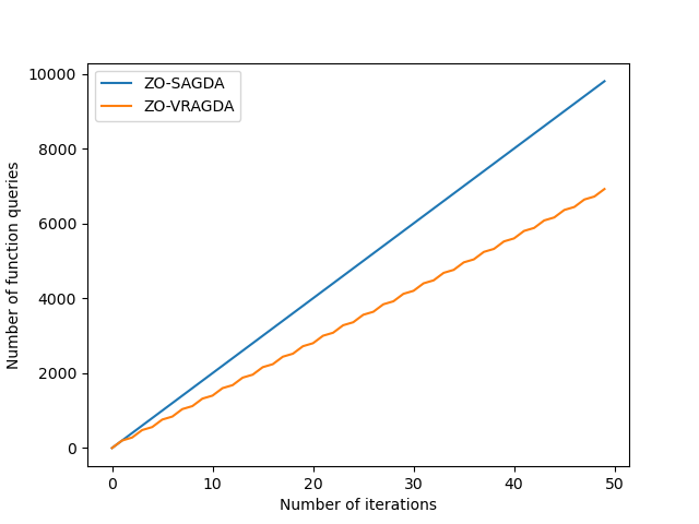
We compare ZO-SAGDA algorithm and ZO-VRAGDA algorithm with the SAGDA algorithm (Yang et al. 2022), which is a first-order algorithm. Set $B=50$ for all three tested algorithms. We set $q=2$ , $b=10$ , $\alpha=0.1$ , $\beta=0.1$ in ZO-VRAGDA, $\alpha=0.1$ , $\beta=0.1$ in ZO-SAGDA and $\tau_{1}=0.1$ , $\tau_{2}=0.1$ in SAGDA respectively. Note that, for ZO-SAGDA algorithm and ZO-VRAGDA algorithm, instead of the exact function value, we use the noisy function value with an additional normal distribution random noise with mean $0$ and variance $0.5$ at each iteration.

Figure 2 shows the average minimum achieved regret function value and the number of function queries up to the $t$ th iteration over 5 independent runs, which is the same as that used in (Liu et al. 2020). From Figure 2, we can find that the performance of ZO-SAGDA algorithm and ZO-VRAGDA algorithm is similar to that of SAGDA algorithm, which is a first order algorithm. Moreover, the number of function value computation of ZO-VRAGDA algorithm is much less than that of ZO-SAGDA algorithm at each iteration.

6 Conclusions and Discussions

In this paper, we propose a zeroth-order alternating gradient descent ascent (ZO-AGDA) algorithm and a zeroth-order variance reduced alternating gradient descent ascent (ZO-VRAGDA) algorithm for solving a class of nonconvex-nonconcave minimax problems, i.e., NC-PL minimax problem, under the deterministic and the stochastic setting respectively. The total number of function value queries to obtain an $\epsilon$ -stationary point of ZO-AGDA and ZO-VRAGDA algorithm for solving NC-PL minimax problem is upper bounded by $\mathcal{O}(\varepsilon^{-2})$ and $\mathcal{O}(\varepsilon^{-3})$ respectively, both of which match the iteration complexity of the corresponding first-order algorithms. To the best of our knowledge, ZO-AGDA and ZO-VRAGDA are the first two zeroth-order algorithms with the complexity gurantee for solving NC-PL minimax problems. Our numerical results further demonstrate the efficiency of the proposed algorithms which approximate the performance of the corresponding first-order algorithms.

Furthermore, note that there is another zeroth-order gradient estimator based on Gaussian smoothing technique that proposed in (Nesterov and Spokoiny 2017) which can be used to estimate the true gradient similar as that in (3) and (4). For the corresponding algorithms, we also can obtain the same total complexity result with Theorem 6 and Theorem 12 that shown in Section 3 and Section 4 respectively. For the brevity of the article, we omit the detailed proofs.

For more general nonconvex-nonconcave minimax problems that the PL conditions are not satisfied, it is worthy of further in-depth study whether the iteration complexity of the proposed algorithm can be guaranteed or not.

References

Allen-Zhu (2017) Zeyuan Allen-Zhu. Natasha: Faster non-convex stochastic optimization via strongly non-convex parameter. In International Conference on Machine Learning, pages 89–97. PMLR, 2017.
Allen-Zhu and Hazan (2016) Zeyuan Allen-Zhu and Elad Hazan. Variance reduction for faster non-convex optimization. In International conference on machine learning, pages 699–707. PMLR, 2016.
Arjovsky et al. (2017) Martin Arjovsky, Soumith Chintala, and Léon Bottou. Wasserstein generative adversarial networks. In International conference on machine learning, pages 214–223. PMLR, 2017.
Bertsimas et al. (2010) Dimitris Bertsimas, Omid Nohadani, and Kwong Meng Teo. Robust optimization for unconstrained simulation-based problems. Operations research, 58(1):161–178, 2010.
Bravo et al. (2018) Mario Bravo, David Leslie, and Panayotis Mertikopoulos. Bandit learning in concave n-person games. Advances in Neural Information Processing Systems, 31, 2018.
Chambolle and Pock (2016) Antonin Chambolle and Thomas Pock. On the ergodic convergence rates of a first-order primal–dual algorithm. Mathematical Programming, 159(1):253–287, 2016.
Chen et al. (2017) Pin-Yu Chen, Huan Zhang, Yash Sharma, Jinfeng Yi, and Cho-Jui Hsieh. Zoo: Zeroth order optimization based black-box attacks to deep neural networks without training substitute models. In Proceedings of the 10th ACM workshop on artificial intelligence and security, pages 15–26, 2017.
Daskalakis and Panageas (2018) Constantinos Daskalakis and Ioannis Panageas. The limit points of (optimistic) gradient descent in min-max optimization. Advances in neural information processing systems, 31, 2018.
Daskalakis et al. (2017) Constantinos Daskalakis, Andrew Ilyas, Vasilis Syrgkanis, and Haoyang Zeng. Training gans with optimism. arXiv preprint arXiv:1711.00141, 2017.
Defazio et al. (2014) Aaron Defazio, Francis Bach, and Simon Lacoste-Julien. Saga: A fast incremental gradient method with support for non-strongly convex composite objectives. Advances in neural information processing systems, 27, 2014.
Fang et al. (2018) Cong Fang, Chris Junchi Li, Zhouchen Lin, and Tong Zhang. Spider: Near-optimal non-convex optimization via stochastic path-integrated differential estimator. Advances in Neural Information Processing Systems, 31, 2018.
Fazel et al. (2018) Maryam Fazel, Rong Ge, Sham Kakade, and Mehran Mesbahi. Global convergence of policy gradient methods for the linear quadratic regulator. In International Conference on Machine Learning, pages 1467–1476. PMLR, 2018.
Finlay and Oberman (2019) Chris Finlay and Adam M Oberman. Scaleable input gradient regularization for adversarial robustness. arXiv preprint arXiv:1905.11468, 2019.
Gao et al. (2018) Xiang Gao, Bo Jiang, and Shuzhong Zhang. On the information-adaptive variants of the admm: an iteration complexity perspective. Journal of Scientific Computing, 76(1):327–363, 2018.
Ghadimi et al. (2016) Saeed Ghadimi, Guanghui Lan, and Hongchao Zhang. Mini-batch stochastic approximation methods for nonconvex stochastic composite optimization. Mathematical Programming, 155(1-2):267–305, 2016.
Gidel et al. (2018) Gauthier Gidel, Hugo Berard, Gaëtan Vignoud, Pascal Vincent, and Simon Lacoste-Julien. A variational inequality perspective on generative adversarial networks. arXiv preprint arXiv:1802.10551, 2018.
Ho and Ermon (2016) Jonathan Ho and Stefano Ermon. Generative adversarial imitation learning. Advances in neural information processing systems, 29, 2016.
Huang et al. (2020) Feihu Huang, Shangqian Gao, Jian Pei, and Heng Huang. Accelerated zeroth-order momentum methods from mini to minimax optimization. arXiv preprint arXiv:2008.08170, 3, 2020.
Huang et al. (2021) Feihu Huang, Xidong Wu, and Heng Huang. Efficient mirror descent ascent methods for nonsmooth minimax problems. Advances in Neural Information Processing Systems, 34:10431–10443, 2021.
Ji et al. (2019) Kaiyi Ji, Zhe Wang, Yi Zhou, and Yingbin Liang. Improved zeroth-order variance reduced algorithms and analysis for nonconvex optimization. In International conference on machine learning, pages 3100–3109. PMLR, 2019.
Johnson and Zhang (2013) Rie Johnson and Tong Zhang. Accelerating stochastic gradient descent using predictive variance reduction. Advances in neural information processing systems, 26, 2013.
Karimi et al. (2016) Hamed Karimi, Julie Nutini, and Mark Schmidt. Linear convergence of gradient and proximal-gradient methods under the polyak-łojasiewicz condition. In Joint European conference on machine learning and knowledge discovery in databases, pages 795–811. Springer, 2016.
Kingma and Ba (2014) Diederik P Kingma and Jimmy Ba. Adam: A method for stochastic optimization. arXiv preprint arXiv:1412.6980, 2014.
Kong and Monteiro (2021) Weiwei Kong and Renato DC Monteiro. An accelerated inexact proximal point method for solving nonconvex-concave min-max problems. SIAM Journal on Optimization, 31(4):2558–2585, 2021.
Letcher et al. (2019) Alistair Letcher, David Balduzzi, Sébastien Racaniere, James Martens, Jakob Foerster, Karl Tuyls, and Thore Graepel. Differentiable game mechanics. The Journal of Machine Learning Research, 20(1):3032–3071, 2019.
Lin et al. (2020a) Tianyi Lin, Chi Jin, and Michael Jordan. On gradient descent ascent for nonconvex-concave minimax problems. In International Conference on Machine Learning, pages 6083–6093. PMLR, 2020a.
Lin et al. (2020b) Tianyi Lin, Chi Jin, and Michael I Jordan. Near-optimal algorithms for minimax optimization. In Conference on Learning Theory, pages 2738–2779. PMLR, 2020b.
Liu et al. (2022) Chaoyue Liu, Libin Zhu, and Mikhail Belkin. Loss landscapes and optimization in over-parameterized non-linear systems and neural networks. Applied and Computational Harmonic Analysis, 59:85–116, 2022.
Liu et al. (2020) Sijia Liu, Songtao Lu, Xiangyi Chen, Yao Feng, Kaidi Xu, Abdullah Al-Dujaili, Mingyi Hong, and Una-May O’Reilly. Min-max optimization without gradients: Convergence and applications to black-box evasion and poisoning attacks. In International conference on machine learning, pages 6282–6293. PMLR, 2020.
Lu et al. (2020) Songtao Lu, Ioannis Tsaknakis, Mingyi Hong, and Yongxin Chen. Hybrid block successive approximation for one-sided non-convex min-max problems: algorithms and applications. IEEE Transactions on Signal Processing, 68:3676–3691, 2020.
Luo et al. (2020) Luo Luo, Haishan Ye, Zhichao Huang, and Tong Zhang. Stochastic recursive gradient descent ascent for stochastic nonconvex-strongly-concave minimax problems. Advances in Neural Information Processing Systems, 33:20566–20577, 2020.
Mokhtari et al. (2020) Aryan Mokhtari, Asuman Ozdaglar, and Sarath Pattathil. A unified analysis of extra-gradient and optimistic gradient methods for saddle point problems: Proximal point approach. In International Conference on Artificial Intelligence and Statistics, pages 1497–1507. PMLR, 2020.
Nemirovski (2004) Arkadi Nemirovski. Prox-method with rate of convergence o (1/t) for variational inequalities with lipschitz continuous monotone operators and smooth convex-concave saddle point problems. SIAM Journal on Optimization, 15(1):229–251, 2004.
Nesterov (2007) Yurii Nesterov. Dual extrapolation and its applications to solving variational inequalities and related problems. Mathematical Programming, 109(2):319–344, 2007.
Nesterov and Spokoiny (2017) Yurii Nesterov and Vladimir Spokoiny. Random gradient-free minimization of convex functions. Foundations of Computational Mathematics, 17(2):527–566, 2017.
Nguyen et al. (2017a) Lam M Nguyen, Jie Liu, Katya Scheinberg, and Martin Takáč. Sarah: A novel method for machine learning problems using stochastic recursive gradient. In International Conference on Machine Learning, pages 2613–2621. PMLR, 2017a.
Nguyen et al. (2017b) Lam M Nguyen, Jie Liu, Katya Scheinberg, and Martin Takáč. Stochastic recursive gradient algorithm for nonconvex optimization. arXiv preprint arXiv:1705.07261, 2017b.
Nguyen et al. (2021) Lam M Nguyen, Katya Scheinberg, and Martin Takáč. Inexact sarah algorithm for stochastic optimization. Optimization Methods and Software, 36(1):237–258, 2021.
Nouiehed et al. (2019) Maher Nouiehed, Maziar Sanjabi, Tianjian Huang, Jason D Lee, and Meisam Razaviyayn. Solving a class of non-convex min-max games using iterative first order methods. Advances in Neural Information Processing Systems, 32, 2019.
Ostrovskii et al. (2021) Dmitrii M Ostrovskii, Andrew Lowy, and Meisam Razaviyayn. Efficient search of first-order nash equilibria in nonconvex-concave smooth min-max problems. SIAM Journal on Optimization, 31(4):2508–2538, 2021.
Pan et al. (2021) Weiwei Pan, Jingjing Shen, and Zi Xu. An efficient algorithm for nonconvex-linear minimax optimization problem and its application in solving weighted maximin dispersion problem. Computational Optimization and Applications, 78(1):287–306, 2021.
Polyak (1963) Boris Teodorovich Polyak. Gradient methods for minimizing functionals. Zhurnal Vychislitel’noi Matematiki i Matematicheskoi Fiziki, 3(4):643–653, 1963.
Rafique et al. (2021) Hassan Rafique, Mingrui Liu, Qihang Lin, and Tianbao Yang. Weakly-convex–concave min–max optimization: provable algorithms and applications in machine learning. Optimization Methods and Software, pages 1–35, 2021.
Reddi et al. (2016) Sashank J Reddi, Ahmed Hefny, Suvrit Sra, Barnabás Póczos, and Alex Smola. Stochastic variance reduction for nonconvex optimization. In International conference on machine learning, pages 314–323. PMLR, 2016.
Shen et al. (2022) Jingjing Shen, Ziqi Wang, and Zi Xu. Zeroth-order single-loop algorithms for nonconvex-linear minimax problems. Journal of Global Optimization, pages 1–30, 2022.
Snoek et al. (2012) Jasper Snoek, Hugo Larochelle, and Ryan P Adams. Practical bayesian optimization of machine learning algorithms. Advances in neural information processing systems, 25, 2012.
Thekumparampil et al. (2019) Kiran K Thekumparampil, Prateek Jain, Praneeth Netrapalli, and Sewoong Oh. Efficient algorithms for smooth minimax optimization. Advances in Neural Information Processing Systems, 32, 2019.
Tieleman et al. (2012) Tijmen Tieleman, Geoffrey Hinton, et al. Lecture 6.5-rmsprop: Divide the gradient by a running average of its recent magnitude. COURSERA: Neural networks for machine learning, 4(2):26–31, 2012.
Wai et al. (2019) Hoi-To Wai, Mingyi Hong, Zhuoran Yang, Zhaoran Wang, and Kexin Tang. Variance reduced policy evaluation with smooth function approximation. Advances in Neural Information Processing Systems, 32, 2019.
Wang et al. (2018) Zhe Wang, Kaiyi Ji, Yi Zhou, Yingbin Liang, and Vahid Tarokh. Spiderboost: A class of faster variance-reduced algorithms for nonconvex optimization. arXiv, 2018, 2018.
Wang et al. (2020) Zhongruo Wang, Krishnakumar Balasubramanian, Shiqian Ma, and Meisam Razaviyayn. Zeroth-order algorithms for nonconvex minimax problems with improved complexities. arXiv preprint arXiv:2001.07819, 2020.
Xu et al. (2020) Tengyu Xu, Zhe Wang, Yingbin Liang, and H Vincent Poor. Enhanced first and zeroth order variance reduced algorithms for min-max optimization. 2020.
Xu et al. (2023a) Zi Xu, Ziqi Wang, Jingjing Shen, and Yuhong Dai. Derivative-free alternating projection algorithms for general nonconvex-concave minimax problems. arXiv preprint arXiv:2108.00473, 2023a.
Xu et al. (2023b) Zi Xu, Huiling Zhang, Yang Xu, and Guanghui Lan. A unified single-loop alternating gradient projection algorithm for nonconvex-concave and convex-nonconcave minimax problems. Mathematical Programming, 2023b. doi: https://doi.org/10.1007/s10107-022-01919-z.
Yang et al. (2020a) Junchi Yang, Negar Kiyavash, and Niao He. Global convergence and variance-reduced optimization for a class of nonconvex-nonconcave minimax problems. arXiv preprint arXiv:2002.09621, 2020a.
Yang et al. (2020b) Junchi Yang, Siqi Zhang, Negar Kiyavash, and Niao He. A catalyst framework for minimax optimization. Advances in Neural Information Processing Systems, 33:5667–5678, 2020b.
Yang et al. (2022) Junchi Yang, Antonio Orvieto, Aurelien Lucchi, and Niao He. Faster single-loop algorithms for minimax optimization without strong concavity. In International Conference on Artificial Intelligence and Statistics, pages 5485–5517. PMLR, 2022.
Zhang et al. (2020) Jiawei Zhang, Peijun Xiao, Ruoyu Sun, and Zhiquan Luo. A single-loop smoothed gradient descent-ascent algorithm for nonconvex-concave min-max problems. Advances in Neural Information Processing Systems, 33:7377–7389, 2020.

		$\displaystyle\quad\mathbb{E}f(x_{t+1},y_{t+1})-\mathbb{E}f(x_{t},y_{t})$
		$\displaystyle\geqslant\beta\mathbb{E}\langle\nabla_{y}f(x_{t+1},y_{t}),\nabla_{y}f(x_{t},y_{t})\rangle-\frac{l}{2}\beta^{2}\mathbb{E}\\|w_{t}\\|^{2}$
		$\displaystyle\quad-\alpha\mathbb{E}\langle\nabla_{x}f(x_{t},y_{t}),\nabla_{x}f_{\mu}(x_{t},y_{t})\rangle-\frac{l}{2}\alpha^{2}\mathbb{E}\\|s_{t}\\|^{2}$
		$\displaystyle=\frac{\beta}{2}\mathbb{E}\\|\nabla_{y}f(x_{t+1}y_{t})\\|^{2}-\frac{\beta}{2}\mathbb{E}\\|\nabla_{y}f(x_{t+1,}y_{t})-\nabla_{y}f_{\mu}(x_{t+1},y_{t})\\|^{2}$
		$\displaystyle\quad+\frac{\beta}{2}\mathbb{E}\\|\nabla_{y}f_{\mu}(x_{t+1},y_{t})\\|^{2}-\frac{l}{2}\beta^{2}\mathbb{E}\\|w_{t}\\|^{2}+\frac{\alpha}{2}\mathbb{E}\\|\nabla_{x}f(x_{t},y_{t})-\nabla_{x}f_{\mu}(x_{t},y_{t})\\|^{2}$
		$\displaystyle\quad-\frac{\alpha}{2}\mathbb{E}\\|\nabla_{x}f(x_{t},y_{t})\\|^{2}-\frac{\alpha}{2}\mathbb{E}\\|\nabla_{x}f_{\mu}(x_{t},y_{t})\\|^{2}-\frac{l}{2}\alpha^{2}\mathbb{E}\\|s_{t}\\|^{2},$		(16)

		$\displaystyle\mathbb{E}\Phi(x_{t+1})-\mathbb{E}\Phi(x_{t})$
		$\displaystyle\leqslant-\alpha\mathbb{E}\langle\nabla\Phi(x_{t}),\nabla_{x}f_{\mu}(x_{t},y_{t})\rangle+\frac{L}{2}\alpha^{2}\mathbb{E}\\|s_{t}\\|^{2}$
		$\displaystyle=\frac{\alpha}{2}\mathbb{E}\\|\nabla\Phi(x_{t})-\nabla_{x}f_{\mu}(x_{t},y_{t})\\|^{2}$		(17)
		$\displaystyle\quad-\frac{\alpha}{2}\mathbb{E}\\|\nabla\Phi(x_{t})\\|^{2}-\frac{\alpha}{2}\mathbb{E}\\|\nabla_{x}f_{\mu}(x_{t},y_{t})\\|^{2}+\frac{L}{2}\alpha^{2}\mathbb{E}\\|s_{t}\\|^{2}$
		$\displaystyle\leqslant\alpha\mathbb{E}\\|\nabla\Phi(x_{t})-\nabla_{x}f(x_{t},y_{t})\\|^{2}+\alpha\mathbb{E}\\|\nabla_{x}f(x_{t},y_{t})-\nabla_{x}f_{\mu}(x_{t},y_{t})\\|^{2}$
		$\displaystyle\quad-\frac{\alpha}{2}\mathbb{E}\\|\nabla\Phi(x_{t})\\|^{2}-\frac{\alpha}{2}\mathbb{E}\\|\nabla_{x}f_{\mu}(x_{t},y_{t})\\|^{2}+\frac{L}{2}\alpha^{2}\mathbb{E}\\|s_{t}\\|^{2}$
		$\displaystyle\leqslant\alpha\kappa^{2}\\|\nabla_{y}f(x_{t},y_{t})\\|^{2}+\alpha\mathbb{E}\\|\nabla_{x}f(x_{t},y_{t})-\nabla_{x}f_{\mu}(x_{t},y_{t})\\|^{2}$
		$\displaystyle\quad-\frac{\alpha}{2}\mathbb{E}\\|\nabla\Phi(x_{t})\\|^{2}-\frac{\alpha}{2}\mathbb{E}\\|\nabla_{x}f_{\mu}(x_{t},y_{t})\\|^{2}+\frac{L}{2}\alpha^{2}\mathbb{E}\\|s_{t}\\|^{2},$		(18)

	$\displaystyle\mathbb{E}V_{t}-\mathbb{E}V_{t+1}$
$\displaystyle\geqslant$	$\displaystyle\frac{3\alpha}{4}\mathbb{E}\\|\nabla\Phi(x_{t})\\|^{2}+\frac{3\alpha}{4}\mathbb{E}\\|\nabla_{x}f_{\mu}(x_{t},y_{t})\\|^{2}$
	$\displaystyle-\frac{3L}{4}\alpha^{2}\mathbb{E}\\|s_{t}\\|^{2}-\frac{3\alpha}{2}\kappa^{2}\mathbb{E}\\|\nabla_{y}f(x_{t},y_{t})\\|^{2}$
	$\displaystyle-\frac{3\alpha}{2}\mathbb{E}\\|\nabla_{x}f(x_{t},y_{t})-\nabla_{x}f_{\mu}(x_{t},y_{t})\\|^{2}+\frac{\beta}{4}\mathbb{E}\\|\nabla_{y}f(x_{t+1},y_{t})\\|^{2}$
	$\displaystyle-\frac{l^{2}}{4}\beta^{2}\mathbb{E}\\|\omega_{t}\\|^{2}-\frac{\alpha}{4}\mathbb{E}\\|\nabla_{x}f_{\mu}(x_{t},y_{t})\\|^{2}-\frac{l}{4}\alpha^{2}\mathbb{E}\\|s_{t}\\|^{2}$
	$\displaystyle-\frac{\beta}{4}\mathbb{E}\\|\nabla_{y}f(x_{t+1},y_{t})-\nabla_{y}f_{\mu}(x_{t+1},y_{t})\\|^{2}-\frac{\alpha}{4}\mathbb{E}\\|\nabla_{x}f(x_{t},y_{t})\\|^{2}$
$\displaystyle\geqslant$	$\displaystyle\frac{3\alpha}{4}\mathbb{E}\\|\nabla\Phi(x_{t})\\|^{2}+\frac{\alpha}{2}\mathbb{E}\\|\nabla_{x}f_{\mu}(x_{t},y_{t})\\|^{2}-L\alpha^{2}\mathbb{E}\\|s_{t}\\|^{2}$
	$\displaystyle-\frac{3\alpha}{2}\kappa^{2}\mathbb{E}\\|\nabla_{y}f(x_{t},y_{t})\\|^{2}-\frac{3\alpha}{2}\mathbb{E}\\|\nabla_{x}f(x_{t},y_{t})-\nabla_{x}f_{\mu}(x_{t},y_{t})\\|^{2}$
	$\displaystyle+(\frac{\beta}{4}-\frac{\beta^{2}}{2}d_{2}L)\mathbb{E}\\|\nabla_{y}f(x_{t+1},y_{t})\\|^{2}-\frac{\beta}{4}\mathbb{E}\\|\nabla_{y}f(x_{t+1},y_{t})-\nabla_{y}f_{\mu}(x_{t+1},y_{t})\\|^{2}$
	$\displaystyle-\frac{\alpha}{4}\mathbb{E}\\|\nabla_{x}f(x_{t},y_{t})\\|^{2}-\frac{L^{3}}{8}\beta^{2}\mu_{2}^{2}d_{2}^{2},$	(19)

	$\displaystyle\\|\nabla_{x}f(x_{t},y_{t})\\|^{2}$	$\displaystyle\leqslant 2\\|\nabla_{x}f(x_{t},y_{t})-\nabla\Phi(x_{t})\\|^{2}+2\\|\nabla\Phi(x_{t})\\|^{2}$
		$\displaystyle\leqslant 2\kappa^{2}\\|\nabla_{y}f(x_{t},y_{t})\\|^{2}+2\\|\nabla\Phi(x_{t})\\|^{2}.$		(20)

	$\displaystyle\\|\nabla_{y}f(x_{t+1},y_{t})\\|^{2}$	$\displaystyle\geqslant\frac{1}{2}\\|\nabla_{y}f(x_{t},y_{t})\\|^{2}-\\|\nabla_{y}f(x_{t+1},y_{t})-\nabla_{y}f(x_{t},y_{t})\\|^{2}$
		$\displaystyle\geqslant\frac{1}{2}\\|\nabla_{y}f(x_{t},y_{t})\\|^{2}-l^{2}\alpha^{2}\\|s_{t}\\|^{2}.$		(21)