Sampling strategies for the Herman–Kluk propagator of the wavefunctionPreprint: AIP/123-QED
Abstract
When the semiclassical Herman–Kluk propagator is used for evaluating quantum-mechanical observables or time-correlation functions, the initial conditions for the guiding trajectories are typically sampled from the Husimi density. Here, we employ this propagator to evolve the wavefunction itself. We investigate two grid-free strategies for the initial sampling of the Herman–Kluk propagator applied to the wavefunction and validate the resulting time-dependent wavefunctions evolved in harmonic and anharmonic potentials. In particular, we consider Monte Carlo quadratures based either on the initial Husimi density or on its square root as possible and most natural sampling densities. We prove analytical convergence error estimates and validate them with numerical experiments on the harmonic oscillator and on a series of Morse potentials with increasing anharmonicity. In all cases, sampling from the square root of Husimi density leads to faster convergence of the wavefunction.
I Introduction
Semiclassical initial value representation techniquesMiller 1970; Miller 2001 have evolved into useful tools for calculations of the dynamics of atoms and molecules.Heller 2018 Frozen Gaussians and their superposition were introducedHeller 1981 by Heller in 1981 as an extension to the thawed Gaussian approximationHeller 1975 in order to capture nonlinear spreading of the wavepackets. Herman and Kluk justified the frozen-Gaussian ansatz and introduced a refined approximation,Herman and Kluk 1984; Herman 1986 now known as the Herman–Kluk propagator, which contains an additional prefactor that rigorously compensates for the fixed width of these frozen Gaussians.
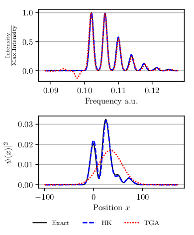
In the spirit of the semiclassical initial value representation, the Herman–Kluk propagator avoids the root search problem.Miller 2001; Kay 2005 Because of its high accuracy, this propagator belongs among the most successful semiclassical approximationsKay 1994a; Walton and Manolopoulos 1996; Garashchuk and Tannor 1996; Thoss and Wang 2004; Spanner et al. 2005; Tatchen and Pollak 2009; Ceotto et al. 2009a and has been derived in many different ways.Kay 1994b; Miller 2002a; Miller 2002b; Shalashilin and Child 2004; Deshpande and Ezra 2006 There are observables, such as low-resolution vibronic spectra in mildly anharmonic systems, which can be well described by the more efficient thawed Gaussian approximation Tannor and Heller 1982; Begušić et al. 2018 and other single-trajectory methods.Hagedorn 1980; Lee and Heller 1982; Hagedorn 1998; Coalson and Karplus 1990; Begušić et al. 2019; Prlj et al. 2020 In chaotic and other systems, however, increased anharmonicity leads to wavepacket splitting and nontrivial interference effects. In such situations, the single-trajectory methods break down, whereas the Herman–Kluk propagator often remains accurate and, at the least, provides a qualitatively correct insight (see, e.g., Fig. 1).
The multi-trajectory nature of the Herman–Kluk propagator is not only its advantage, but also its bottleneck. In particular, converged computations might require an extremely large number of trajectories. For this reason, several groups designed various methods, whose goal is reducing the number of trajectories required by the Herman–Kluk propagator. These include, e.g., Filinov filtering,Filinov 1986; Makri and Miller 1987; Makri and Miller 1988; Walton and Manolopoulos 1996, time-averaging,Elran and Kay 1999; Kaledin and Miller 2003; Buchholz et al. 2016; Buchholz et al. 2018, semiclassical interaction picture,Shao and Makri 2000; Petersen and Pollak 2015 multiple-coherent states,Ceotto et al. 2009b, hybrid dynamics,Grossmann 2006; Goletz and Grossmann 2009; Grossmann 2016 mixed quantum-semiclassical dynamics,Antipov et al. 2015; Church et al. 2017; Malpathak et al. 2022 and many others, which achieve the reduction in the number of trajectories by applying one of several possible further approximations.
Yet, the number of guiding trajectories can already be significantly reduced simply by choosing the sampling density of the initial conditions wisely. Although the acceleration of the convergence may be smaller than with the previously mentioned methods, the advantage of this approach is that the converged results agree exactly with the converged results of the original Herman–Kluk propagator. For this reason, most calculations of observables, time-correlation functions, and wavepacket autocorrelation functions, i.e., quantities quadratic in the wavefunction, correctly employ sampling from the Husimi density of the initial state.Miller 2001; Pollak et al. 2022 In contrast, the choice of the optimal sampling density for the Herman–Kluk wavefunction itself has not been analyzed in detail.
The goal of this work is, therefore, to analyze the convergence of the Herman–Kluk wavefunction for different initial sampling strategies and to understand the convergence error as a function of time. Specifically, we investigate two mesh-free discretization approaches for the initial sampling—first analytically and then numerically on the examples of harmonic and Morse oscillators with increasing anharmonicity.
The remainder of this paper is organized as follows. In the next section we briefly introduce the Herman–Kluk propagator and its components necessary for numerical computations. We define the initial sampling densities and specify the algorithm used for numerical experiments. In the main Sec. 3, we analyze the errors at the initial and final times due to the phase-space discretization. In particular, we prove that in the harmonic oscillator this error is a periodic function of time. Our numerical experiments in Sec. 4 confirm the theoretical error estimates and provide further insights into the anharmonic evolution generated by Morse potentials, which are not accessible to explicit analytical calculations.
II Discretising the Herman–Kluk propagator
II.1 Herman–Kluk propagator
Evolution of a quantum state is governed by the time-dependent Schrödinger equation
| (1) |
where is the reduced Planck constant and is the Hamiltonian operator. Here, we assume the Hamiltonian to be the time-independent operator
| (2) |
where is the mass (after mass-scaling coordinates), and and are -dimensional position and momentum vectors. Under the usual regularity and growth assumptions on the potential energy function , the spectral-theorem Hall 2013 provides for all times a well-defined unitary propagator
| (3) |
in terms of which the solution of (1) can be expressed as
| (4) |
for all square integrable initial data .
Solving the Schrödinger equation numerically is notoriously difficult for various reasons. With respect to the atomic scale, the nuclear mass is rather large, so that the presence of the factor in the kinetic energy operator induces highly oscillatory motion both with respect to time and space. More importantly, for most molecular systems the dimension of the configuration space is so large that grid-based integration methods are very expensive if not infeasible. Therefore, one often resorts to mesh-free discretization methods or semiclassical approximations, both of which alleviate this “curse of dimensionality” at least partially.
The semiclassical Herman–Kluk propagator utilizes frozen Gaussian functions
| (5) | ||||
with a centre at the phase-space point and with a fixed, real, symmetric, positive-definite width-matrix . The frozen Gaussians form an over-complete subset of the Hilbert space of square integrable functions. They have the striking property that any can be decomposed asMartinez 2002
| (6) |
with the scaled phase-space measure Using this decomposition for our solution of the time-dependent Schrödinger equation, we obtain
| (7) |
Based on the continuous superposition (7), the state obtained by applying the Herman–Kluk propagator to can be expressed as
| (8) |
where is the solution to the underlying classical Hamiltonian system
| (9) |
for the Hamiltonian function , where
| (10) |
is the standard symplectic matrix. denotes the classical action integral
| (11) |
which solves the initial value problem
| (12) |
for all In (8), the Herman–Kluk prefactor
| (13) | ||||
depends on the matrices
| (14) |
i.e., the four block components of the stability matrix Stability matrix, defined as the Jacobian of the flow map, is the solution to the variational equation
| (15) |
with the Hessian of the Hamiltonian function .
The Herman–Kluk approximation has been mathematically justified in different works.Kay 2006; Lasser and Lubich 2020; Swart and Rousse 2008; Robert 2010 It has been shown that the exactly evolved quantum state is approximated by the state
| (16) |
obtained by applying the Herman–Kluk propagator to the initial state , with an error of the order of More precisely,
| (17) |
for all initial data of norm one, where is a fixed time and is a constant independent of If the potential is at most harmonic, then the approximation is exact. Lasser and Lubich 2020
II.2 Discretisation
Evolving the wavefunction (8) with the Herman–Kluk propagator requires evaluating an integral over the phase space and the overlap of the initial state with a frozen Gaussian. Furthermore, the algorithm needs to propagate the trajectories the classical action , and the Herman–Kluk prefactor according to Hamilton’s equations of motion for all chosen quadrature points The latter can be achieved using symplectic integration methods to preserve also the symplectic structure of the classical Hamiltonian system. Due to the curse of dimensionality, for high the integral on must be evaluated using mesh-free discretization, such as Monte Carlo methods. Caflisch 1998
To evaluate the Herman–Kluk wavefunction by Monte Carlo sampling, we rewrite the integral from Eq. 8 as
| (18) |
where we introduced the notation
| (19) | ||||
for the phase-space average of with respect to a probability measure with density and defined a time-dependent state
| (20) |
i.e., a propagated frozen Gaussian multiplied by the Herman–Kluk and phase prefactors, and a time-independent function
| (21) |
The Monte Carlo estimator is then given by
| (22) |
where is the state obtained from initial condition and are sampled from probability density .
As for any importance sampling, there are infinitely many ways to decompose the time-independent part of the phase space integrand in Eq. 8 into the product of a prefactor with a normalized sampling density . If one computes observables and correlation functions, which are quadratic in the initial state, is typically taken to be the Husimi probability density
| (23) |
of the initial state . For Husimi distribution, the prefactor becomes
| (24) |
However, since the wavefunction evolved with the Herman–Kluk propagator is first- and not second-order in , it is natural to also test the square root of the Husimi density and to consider the probability density
| (25) |
with a bounded prefactor
| (26) |
The two probability densities and can now be used to compute the phase-space integral by Monte Carlo integration. To sum up, we have two cases, in which we evaluate either as
| (Case H) |
or as
| (Case sqrt-H) |
In general, the integral over defining the overlap of the initial wavefunction with a Gaussian has to be computed by numerical quadrature. However, for important specific cases analytical formulas are available. If the initial wavefunction is a Gaussian wavepacket centred at some phase-space point , then
| (27) | ||||
where is the matrix containing the width parameters of the initial coherent state. Then, the Husimi density is given by
| (28) |
whereas the second approach provides the density
| (29) |
and prefactor
| (30) |
II.3 Summary of the numerical algorithm
Taking into account all the previous considerations, we slightly extend the natural numerical algorithm (described, e.g., in Ref. Lasser and Sattlegger 2017, Sec. 4]) for finding the Herman–Kluk approximation to the wavefunction at time :
Algorithm 1.
(Herman–Kluk propagation)
- 1.
- 2.
For all
- 2.1
Set initial values and
- 2.2
Compute approximate solutions to Eqs. 9, 12 and 15 up to time with a symplectic integration methodBrewer et al. 1997 based on the Störmer–Verlet scheme. Hairer et al. 2006; Hairer et al. 2003
- 2.3
Compute the Herman–Kluk prefactor from while choosing the correct branch of the complex square root,Stewart and Tall 2018 which guarantees continuity of as a function of .
- 2.1
- 3.
We note that Eqs. 9, 12 and 15 can be evaluated simultaneously with a single numerical integrator. To increase the accuracy of the time integration one can use higher-order composition methods.Kahan and Li 1997; Suzuki 1992 They increase the order of the time integrator, but also its numerical cost. A higher-order time integrator is not necessarily useful since the phase-space error occurring from the Monte Carlo quadrature usually dominates the time integration error.
III Phase space error analysis
Algorithm 1 relies on the discretisation of the phase-space integrals and of the system of ordinary differential equations. Here we focus only on the phase-space discretisation error.
III.1 Moments of the integrand
To assess the accuracy of the Monte Carlo estimator (22), we examine the moments of the two different integrands: and First, we observe that for any ,
| (33) |
since and the Herman–Kluk prefactor are both bounded functions. For a discussion of the boundedness of , see Appendix A. In contrast,
| (34) | ||||
ceases to be finite for . However, both integrands have a finite first moment, so that the Strong Law of Large Numbers (Theorem 2.4.1 in Ref. Durrett 2019) provides convergence of the estimator,
| (35) |
with probability one. The non-existing second moment for (Case H) results in a slightly worse convergence rate than the one for (Case sqrt-H). Numerical results in Sec. IV confirm this expectation.
III.2 Mean squared error
For (Case sqrt-H) the second moment is finite, so that the mean squared error of the Monte Carlo estimator (22) is well-defined and satisfies
| (36) |
where the expectation value and the variance are with respect to the density . Moreover, Lasser and Sattlegger 2017
| (37) | ||||
In the special case of an initial Gaussian initial wavepacket , this simplifies to
| (38) |
and at initial time we obtain
| (39) |
since the Herman–Kluk prefactor satisfies .
For a more general assessment of the variance, numerical experiments in Sec. IV consider the error between the approximations with and samples. By the linearity of the expectation value and the triangle inequality, this error can be estimated by
| (40) | ||||
Note that Eq. 36 gives only the expected convergence error, i.e., the convergence error averaged over infinitely many independent simulations, each using trajectories. The actual convergence error for any specific simulation with trajectories may deviate from this analytical estimate substantially due to statistical noise. Nevertheless, in Appendix B, we explain how Eq. 36 can also provide a rigorous lower bound and asymptotic estimate of the number of trajectories needed for convergence of a single simulation.
III.3 Other sampling densities
For the special case of an initial Gaussian wavepacket , the two proposed sampling densities and belong to a family of normal distributions with probability density functions
| (41) |
with . In the spirit of importance sampling, the Herman–Kluk wavefunction can accordingly be written as a phase-space average
| (42) |
At time , the norm of the integrand satisfies
| (43) | ||||
which implies for the variance
| (44) | ||||
For , the function attains its minimum at , which corresponds to the sampling density . In other words, (Case sqrt-H) is optimal as far as the mean squared error is concerned.
III.4 Harmonic motion
The one-dimensional harmonic oscillator
| (45) |
is one of the rare examples for which explicit expressions for the solution of the Schrödinger equation and for the Herman–Kluk prefactor exist. For an initial Gaussian wavepacket with position and momentum the exact wavefunction is given byTannor 2007
| (46) |
where
| (47) | ||||
| (48) | ||||
| (49) | ||||
| (50) |
with the abbreviations and Here, includes the normalization constant for the wavefunction at time The classical action is given by
| (51) | ||||
The four components of stability matrix can be obtained, from their definition (14), by differentiating expressions for and with respect to and , namely
| (52) |
The Herman–Kluk prefactor satisfies
| (53) |
so that the variance (37) can be written as
| (54) | ||||
This implies that for (Case sqrt-H) applied to a harmonic oscillator, the mean squared error of our Monte Carlo estimator oscillates with a period of between
| (55) |
IV Numerical examples
In this section, we complement our previous theoretical results with numerical examples. We start by examining how the performance of Algorithm 1 depends on the method to discretise the phase space. We explore the time dependence of the variance of the Monte Carlo estimator in one dimension in a harmonic oscillator as well as in a series of increasingly anharmonic Morse potentials. The Monte Carlo integration is tested by averaging over independent, identically distributed samples of initial conditions. We approximate its convergence rate by assuming a power law
| (56) |
dependence of the mean statistical error on the number of samples . The prefactor and order of convergence are determined by the linear fit (in the least-squares sense) of the logarithm of Eq. (56) to the dependence of the logarithm of the statistical error on the logarithm of .
Throughout our numerical examples, we work in atomic units mass-scaled coordinates and with an initial state that is a Gaussian wavepacket with phase-space centre
IV.1 Initial phase-space error

We start by considering a spherical initial Gaussian wavepacket with a width parameter in one and four dimensions. For , it is centreed at and for , at . Figure 2 shows the -distance
| (57) |
of the Monte Carlo estimators for (Case H) and (Case sqrt-H) from the exact wavefunction at initial time as a function of the number of Monte Carlo quadrature points. We can immediately see that the analytical prediction (39) of the mean squared error (36) of (Case sqrt-H) is fulfilled. For (Case H), the curve-fitting approximation (56) provided for and for It shows that both cases converge to the correct result and that (Case sqrt-H) performs slightly better than (Case H). Additionally, Fig. 3 displays the -distance of the estimators for both cases from the exact wavefunction at initial time as a function of the dimension Each wavefunction was approximated with trajectories. The analytical prediction (39) for (Case sqrt-H) is realized. Moreover, the error for (Case H) increases faster with .

IV.2 Harmonic potential

To analyze the effect of dynamics on the convergence, let us consider a harmonic potential in one dimension and explore the dynamics for one full oscillation period. The initial Gaussian wavepacket is still localized in with width In Fig. 4, we compare the exact wavefunction (46) with the numerical realization of the Herman–Kluk propagator which uses the exact solution to and stated in Eqs. 48, 49, 51 and 53. Since the Herman–Kluk propagator is exact for harmonic motion and since we supply exact classical trajectories, the observed numerical error is only due to the Monte Carlo integration. The upper panel of Fig. 4 shows the time dependence of the -error
| (58) |
where the semiclassical wavefunctions were generated using trajectories. Sampling from the square root of the Husimi density (Case sqrt-H) results in approximately twice smaller error than sampling from the Husimi density itself. For (Case sqrt-H), the figure also displays the analytical error estimate derived in (54), which matches the numerical error up to small statistical noise. To remove this statistical noise and to match the analytical estimate (54) more accurately, in the lower panel of Fig. 4 we plot the empirical root mean square error (RMSE) Caflisch 1998 , where
| (59) |
is an integer number of independent simulations (indexed by ) and each was itself approximated using independent samples. One can see that
| (60) |
For , one obtains the result represented in the upper panel of Fig. 4. For due to the Strong law of large numbers, converges almost surely to its expectation value and hence to the analytical error estimate.
The lower panel of Fig. 4 shows the empirical RMSE computed with and For (Case sqrt-H), it coincides almost perfectly with the analytical prediction. We note that the error reaches its maximum whenever the wavefunction passes through the bottom of the potential and its minimum when the wavefunction arrives at the turning points. Even though this analysis makes only sense for finite variance, the figure also displays the empirical RMSE for (Case H), which is nearly constant. Both panels show a qualitatively similar error evolution for (Case H), however, at a magnitude that is considerably larger than the error for (Case sqrt-H).
IV.3 Morse potential


To investigate the convergence of the Herman–Kluk wavefunction in anharmonic systems, we consider dynamics generated by a less and more anharmonic Morse potentials. The parameters were taken from [Begušić et al. 2019]. Our initial state is a Gaussian wavepacket with zero initial position and momentum, , and with a width parameter a.u. The Morse potential
| (61) |
is characterized by the dissociation energy , decay parameter , and the position and energy of the minimum. We considered two Morse potentials, both with and a.u., but with different values of and . The latter two parameters, however, were chosen so that the global harmonic potential fitted to the Morse potential at had the same frequency
| (62) |
for the two Morse potentials. The anharmonicity of the potentials was conveniently controlled with the dimensionless parameter
| (63) |
which is also reflected in the bound energy levels Tannor 2007
| (64) |
of a Morse oscillator. Then and are given by
| (65) | ||||
We choose two different values
| (66) |
of anharmonicity and compare the Herman–Kluk propagation with a grid-based reference quantum calculation obtained by the Fourier-split method,Feit and Fleck 1983 that is second-order accurate with respect to the time step. The position grid was set from to with equidistant points for and from to with equidistant points for . The larger grid for was required to capture oscillations of the wavefunctions in the tail region, which are due to the increased anharmonicity. For the time propagation of the Herman–Kluk wavefunction, we used a second order Størmer-Verlet scheme with step size a.u. fs.
Because the Herman–Kluk approximation is not exact in a Morse potential, to separate the statistical convergence error from the semiclassical error of the fully converged Herman–Kluk approximation, in Figure 5 we show the -error
| (67) |
between the Herman–Kluk wavefunctions calculated with and trajectories as a function of . Both wavefunctions were propagated in a Morse potential with anharmonicity . Each panel includes the error for the fixed time after approximately one oscillation timesteps) and ten oscillations timesteps). In addition, the convergence rates for both sampling schemes were fitted to the same power law (56). We observe that sampling from the square root of the Husimi density (Case sqrt-H), shown in the lower panel, performs better than sampling from the Husimi density (Case H), displayed in the upper panel.
Figure 6 shows the analogous results obtained in a Morse potential with a larger anharmonicity parameter Here, we display the wavefunctions after and time steps, which are approximately the times after the first and tenth oscillations. As expected for anharmonic evolution, the error after ten oscillations is worse than after one oscillation. Increased anharmonicity also increases the error in comparison to Fig. 5. Again, the sampling from the square root of the Husimi density (Case sqrt-H) has consistently a lower error than (Case H).
To complement the abstract convergence study of the -error, in the upper panels of Fig. 7 and Fig. 8, we compare the more intuitive position probability densities of the “exact” quantum grid-based solution with those of (Case H) and (Case sqrt-H). Both figures were obtained in a Morse potential with anharmonicity parameter at a time after ten oscillations. The difference lies in the number of trajectories used. The less converged results in Fig. 7 were obtained with only trajectories, whereas the fully converged results in Fig. 8 employed trajectories. The lower panels of the two figures display the absolute errors of the position density for the two cases, measured with respect to the “exact” grid-based position density. The two panels of Fig. 7 confirm again that sampling from the square root of Husimi density (Case sqrt-H) results in faster convergence than sampling from the Husimi density (Case sqrt-H). The upper panel of Fig. 8 shows that in the numerically converged regime, the Herman–Kluk propagator approximates the exact solution in this system very well, regardless whether one samples from the Husimi density or its square root. The fact that results are numerically converged is confirmed in the lower panel of Fig. 8, where the errors of (Case H) and (Case sqrt-H) are approximately the same, which implies that the common remaining error is the error of the Herman–Kluk approximation and not the phase-space discretization error.
Analytical expressions and numerical fits to the convergence rates for all studied systems are summarized in Table 1.
Finally, we note that Fig. 1 in the Introduction was based, as Fig. 8, on the Morse potential with anharmonicity parameter and Herman–Kluk calculations used trajectories. For the computation of the position density, we used the more efficient (Case sqrt-H). The spectra in the upper panel were obtained by the Fourier transform of the wavepacket autocorrelation function; the Herman–Kluk autocorrelation function was computed by sampling from the Husimi density (Case H), because it gives the exact result (=1) at regardless of the number of trajectories and, therefore, converges faster at short times.
V Conclusion and outlook
| (Case sqrt-H) | (Case H) | |
|---|---|---|
| Initial time | ||
| Harmonic pot. | ||
| with variance | ||
| from (54) | ||
| Morse pot.: | ||
| 1 oscillation | ||
| 10 oscillations | ||
| Morse pot.: | ||
| 1 oscillation | ||
| 10 oscillations |
We compared two different sampling strategies for evaluating the semiclassical wavefunction evolved with the Herman–Kluk propagator. For the initial phase-space sampling, we either used the Husimi density (Case H) or its square root (Case sqrt-H). We showed that the square root sampling produces a Monte Carlo integrand with finite second moment, while the Husimi sampling comes with an undesirable infinite second moment. The numerical experiments for the harmonic oscillator and two Morse oscillators with different extents of anharmonicity confirm that the infinite second moment results in a slower convergence of the Monte Carlo estimator. Therefore, we recommend the square root approach (Case sqrt-H) whenever the Herman–Kluk propagator is used directly for approximating the quantum-mechanical wavefunction and the -error of the wavefunction approximation is the relevant accuracy measure. A follow-up paper applying a similar analysis to the autocorrelation function as well as to the expectation values computed with the Herman–Kluk propagator is in preparation.
Acknowledgments
The authors acknowledge financial support from the European Research Council (ERC) under the European Union’s Horizon 2020 Research and Innovation Programme (Grant Agreement No. 683069–MOLEQULE) and from the EPFL.
Appendix A Boundedness of Herman–Kluk prefactor
For notational simplicity we consider the case A general does not change the argument, but it requires to exchange by
| (68) |
in the following. We recall that
| (69) | ||||
with
| (70) |
Following [Lasser and Lubich 2020, Lemma 5.6], for one calculates
| (71) |
Hence,
| (72) | ||||
With this representation, we can link growth and boundedness of directly with growth and boundedness of the stability matrix, and it is the largest eigenvalue of the Hessian that ultimately gives upper bounds on .
Appendix B Number of trajectories needed for convergence
In the following, we give a lower bound as well as an asymptotic estimate for the number of trajectories needed “for convergence,” or, more precisely, needed to guarantee that the probability of the convergence error exceeding a specified threshold is below a prescribed value . The following analysis holds for any potential in any number of dimensions , but assumes that the variance of the estimator is finite.
On one hand, Chebyshev’s inequalityDurrett 2019
| (73) |
implies that the number of trajectories must obey the inequality
| (74) |
in order that the probability of the convergence error exceeding be at most .
On the other hand, the central limit theoremDurrett 2019 states that the random variable
| (75) |
converges in distribution to the standard normally distributed random variable. Hence, the probability for the convergence error to be above this threshold is
| (76) | ||||
For a given probability that is exceeded, this leads to the asymptotic behaviour
| (77) |
where is the complementary error function.Dyke 2013
References
References
- Miller (1970) W. H. Miller, J. Chem. Phys. 53, 3578 (1970).
- Miller (2001) W. H. Miller, J. Phys. Chem. A 105, 2942 (2001).
- Heller (2018) E. J. Heller, The semiclassical way to dynamics and spectroscopy (Princeton University Press, Princeton, NJ, 2018).
- Heller (1981) E. J. Heller, J. Chem. Phys. 75, 2923 (1981).
- Heller (1975) E. J. Heller, J. Chem. Phys. 62, 1544 (1975).
- Herman and Kluk (1984) M. F. Herman and E. Kluk, Chem. Phys. 91, 27 (1984).
- Herman (1986) M. F. Herman, J. Chem. Phys. 85, 2069 (1986).
- Kay (2005) K. G. Kay, Annu. Rev. Phys. Chem. 56, 255 (2005).
- Kay (1994a) K. G. Kay, J. Chem. Phys. 100, 4432 (1994a).
- Walton and Manolopoulos (1996) A. R. Walton and D. E. Manolopoulos, Mol. Phys. 87, 961 (1996).
- Garashchuk and Tannor (1996) S. Garashchuk and D. Tannor, Chem. Phys. Lett. 262, 477 (1996).
- Thoss and Wang (2004) M. Thoss and H. Wang, Annu. Rev. Phys. Chem. 55, 299 (2004).
- Spanner et al. (2005) M. Spanner, V. S. Batista, and P. Brumer, J. Chem. Phys. 122, 084111 (2005).
- Tatchen and Pollak (2009) J. Tatchen and E. Pollak, J. Chem. Phys. 130, 041103 (2009).
- Ceotto et al. (2009a) M. Ceotto, S. Atahan, S. Shim, G. F. Tantardini, and A. Aspuru-Guzik, Phys. Chem. Chem. Phys. 11, 3861 (2009a).
- Kay (1994b) K. G. Kay, J. Chem. Phys. 100, 4377 (1994b).
- Miller (2002a) W. H. Miller, J. Phys. Chem. B 106, 8132 (2002a).
- Miller (2002b) W. H. Miller, Mol. Phys. 100, 397 (2002b).
- Shalashilin and Child (2004) D. V. Shalashilin and M. S. Child, Chem. Phys. 304, 103 (2004).
- Deshpande and Ezra (2006) S. A. Deshpande and G. S. Ezra, J. Phys. A 39, 5067 (2006).
- Tannor and Heller (1982) D. J. Tannor and E. J. Heller, J. Chem. Phys. 77, 202 (1982).
- Begušić et al. (2018) T. Begušić, J. Roulet, and J. Vaníček, J. Chem. Phys. 149, 244115 (2018).
- Hagedorn (1980) G. A. Hagedorn, Commun. Math. Phys. 71, 77 (1980).
- Lee and Heller (1982) S.-Y. Lee and E. J. Heller, J. Chem. Phys. 76, 3035 (1982).
- Hagedorn (1998) G. A. Hagedorn, Ann. Phys. (NY) 269, 77 (1998).
- Coalson and Karplus (1990) R. D. Coalson and M. Karplus, J. Chem. Phys. 93, 3919 (1990).
- Begušić et al. (2019) T. Begušić, M. Cordova, and J. Vaníček, J. Chem. Phys. 150, 154117 (2019).
- Prlj et al. (2020) A. Prlj, T. Begušić, Z. T. Zhang, G. C. Fish, M. Wehrle, T. Zimmermann, S. Choi, J. Roulet, J.-E. Moser, and J. Vaníček, J. Chem. Theory Comput. 16, 2617 (2020).
- Filinov (1986) V. S. Filinov, Nucl. Phys. B 271, 717 (1986).
- Makri and Miller (1987) N. Makri and W. H. Miller, Chem. Phys. Lett. 139, 10 (1987).
- Makri and Miller (1988) N. Makri and W. H. Miller, J. Chem. Phys. 89, 2170 (1988).
- Elran and Kay (1999) Y. Elran and K. G. Kay, J. Chem. Phys. 110, 3653 (1999).
- Kaledin and Miller (2003) A. L. Kaledin and W. H. Miller, J. Chem. Phys. 118, 7174 (2003).
- Buchholz et al. (2016) M. Buchholz, F. Grossmann, and M. Ceotto, J. Chem. Phys. 144, 094102 (2016).
- Buchholz et al. (2018) M. Buchholz, F. Grossmann, and M. Ceotto, J. Chem. Phys. 148, 114107 (2018).
- Shao and Makri (2000) J. Shao and N. Makri, J. Chem. Phys. 113, 3681 (2000).
- Petersen and Pollak (2015) J. Petersen and E. Pollak, J. Chem. Phys. 143, 224114 (2015).
- Ceotto et al. (2009b) M. Ceotto, S. Atahan, G. F. Tantardini, and A. Aspuru-Guzik, J. Chem. Phys. 130, 234113 (2009b).
- Grossmann (2006) F. Grossmann, J. Chem. Phys. 125, 014111 (2006).
- Goletz and Grossmann (2009) C. M. Goletz and F. Grossmann, J. Chem. Phys. 130, 244107 (2009).
- Grossmann (2016) F. Grossmann, Phys. Scr. T 91, 044004 (2016).
- Antipov et al. (2015) S. V. Antipov, Z. Ye, and N. Ananth, J. Chem. Phys. 142, 184102 (2015).
- Church et al. (2017) M. S. Church, S. V. Antipov, and N. Ananth, J. Chem. Phys. 146, 234104 (2017).
- Malpathak et al. (2022) S. Malpathak, M. S. Church, and N. Ananth, J. Phys. Chem. A 126, 6359 (2022).
- Pollak et al. (2022) E. Pollak, S. Upadhyayula, and J. Liu, J. Chem. Phys. 156, 244101 (2022).
- Hall (2013) B. C. Hall, Quantum Theory for Mathematicians (Springer New York, NY, 2013).
- Martinez (2002) A. Martinez, An Introduction to Semiclassical and Microlocal Analysis (Springer-Verlag, New York, 2002).
- Kay (2006) K. G. Kay, Chemical Physics 322, 3 (2006).
- Lasser and Lubich (2020) C. Lasser and C. Lubich, Acta Numerica 29, 229 (2020).
- Swart and Rousse (2008) T. Swart and V. Rousse, Commun. Math. Phys. 286, 725 (2008).
- Robert (2010) D. Robert, Reviews in Mathematical Physics 22, 1123 (2010).
- Caflisch (1998) R. E. Caflisch, Acta Numerica 7, 1– (1998).
- Lasser and Sattlegger (2017) C. Lasser and D. Sattlegger, Numerische Mathematik 137, 119 (2017).
- Brewer et al. (1997) M. L. Brewer, J. S. Hulme, and D. E. Manolopoulos, J. Chem. Phys. 106, 4832 (1997).
- Hairer et al. (2006) E. Hairer, C. Lubich, and G. Wanner, Geometric Numerical Integration: Structure-Preserving Algorithms for Ordinary Differential Equations (Springer Berlin Heidelberg New York, 2006).
- Hairer et al. (2003) E. Hairer, C. Lubich, and G. Wanner, Acta Numerica 12, 399 (2003).
- Stewart and Tall (2018) I. Stewart and D. Tall, Complex Analysis (Cambridge University Press, 2018).
- Kahan and Li (1997) W. Kahan and R.-C. Li, Math. Comput. 66, 1089 (1997).
- Suzuki (1992) M. Suzuki, Phys. Lett. A 165, 387 (1992).
- Durrett (2019) R. Durrett, Probability: Theory and Examples (Cambridge University Press, 2019).
- Tannor (2007) D. J. Tannor, Introduction to Quantum Mechanics: A Time-Dependent Perspective (University Science Books, Sausalito, 2007).
- Feit and Fleck (1983) M. D. Feit and J. A. Fleck, Jr., J. Chem. Phys. 78, 301 (1983).
- Dyke (2013) P. Dyke, An Introduction to Laplace Transforms and Fourier Series (Springer London, 2013).