Cascade infrared thermal photon emission
Abstract
The time development of the excitation energy of molecules and clusters cooling by emission of thermal vibrational infrared radiation has been studied. The energy distributions and the photon emission rates develop into near-universal functions that can be characterized with only a few parameters, irrespective of the precise vibrational spectra and oscillator strengths of the systems. The photon emission constant and emitted power averaged over all thermally populated states vary linearly with total excitation energy with a small offset. The time developments of ensemble internal energy distributions are calculated with respect to their first two moments. For the derived linear dependence of the emission rate constant, these results are exact.
1 Introduction
Emission of photons is an important cooling channel for molecules and clusters in the absence of collisions. The decay channel is becoming increasingly interesting in astrophysical context due to the growing number of molecules observed in interstellar space Herbst and Dishoeck 2009; McGuire 2018. The vastly different frequency factors and activation energies associated with the different thermal processes (fragmentation, thermionic emission, recurrent fluorescence, and infrared (IR) emission) create a hierarchy of time scales on which the possible thermal decay channels of thermally excited molecules proceed. The IR photon emission is located at the lowest energies of this hierarchy, making it the energy-loss channel that will dominate at the latest stage of the cooling process. The development of cryogenic storage rings has opened the possibility to study cooling processes on very long time scales in the laboratory Lange et al. 2012; Najafian et al. 2014; Breitenfeldt et al. 2018; Bull et al. 2019; Stockett et al. 2020; Stockett et al. 2020. The extension of feasible storage times to thousands of seconds in these devices places a special emphasis on the understanding of this long time emission of thermal infrared photons from stored ions Goto et al. 2013; Najafian et al. 2014; Bull et al. 2019; Ferrari et al. 2019; Stockett et al. 2020; Stockett et al. 2020; Iida et al. 2021; D. Muell
Before embarking on such a calculation of rate constants and energy distributions, it is worthwhile to consider two aspects of the thermal description of the vibrational degrees of freedom of a molecule or cluster. One is the question of ergodicity. The low internal energies of the emitting molecules/clusters raise this question with more force than for other decay channels that need higher excitation energies to be sustained. Harmonic oscillators do not couple, and when a collection of rigorously uncoupled harmonic oscillators is used to describe the thermal properties of the vibrational degrees of freedom, each of the modes will cool down independently; clearly, for a system of this type the cooling proceeds independently for all oscillators. The time dependence and average values can be calculated for such a system without any further ado.
However, as molecular vibrations are not harmonic, energy can flow between different vibrational modes, a process know as intramolecular vibrational redistribution (IVR) Bixon and Jortner 1968; Gruebele and Wolynes 2004; Makarov et al. 2012. IVR is indeed an essential component of our understanding of many phenomena at the heart of physical chemistry, such as reaction rate theories, fluorescence and coherent control.
The time scales associated with IVR are determined by the degree of anharmonicity, and scale with the density of states in the simplest large molecule case (see ref. Nesbitt and Field 1996 for an introduction to the subject). These IVR time scales are short enough to make IVR efficient on the timescales of milliseconds and longer, which are the characteristic times of IR radiation. Radiative cooling measurements in storage rings do indeed indicate that IVR is the correct framework to describe the radiation at long times Bull et al. 2019; Stockett et al. 2020; D. Muell. The ’rapid exchange limit’ denotes the case in which IVR is much faster than IR emission, and consequently, all states with the same total internal energy will mix rapidly. We will use the rapid exchange limit Ansatz here.
Another point worth mentioning is the little considered fact that vibrational motion carries angular momentum. The simplest case of linear molecules has been analyzed in Hansen and Ferrari 2021. It is also well-known from the description of the excitation modes of helium droplets Brink and Stringari 1990; Lehmann 2004; Hansen et al. 2007. The conservation of this quantity imposes a constraint on the states that mix in the IVR process. This clearly has consequences also for the photon emission rates. However, a general theory is not yet available for molecules, and an in-depth treatment of the subject is beyond the scope of this article. We will restrict the work here to consider only the case of unrestricted IVR.
Within this framework we will show that vibrational cooling produces an almost linear scaling of the cooling rate constants with the internal energy of the system and, as a consequence, that the photon emission rate constant decays exponentially with time and with a rate constant that can be computed. We will use this scaling to calculate the time development of the general case where energy distributions are not delta functions.
2 The harmonic cascade model
We describe the nuclear vibrations of a molecule with atoms as harmonic oscillators with energies , . In this approximation, which is sufficiently accurate at the low energies we consider, the total excitation energy, , of a molecule is therefore a sum over the mode energies:
| (1) |
where are the number of excitation quanta in mode . A list of these occupation numbers, specifies the system and will be denoted its state. Within the harmonic approximation, IR radiative emission only occurs between neighboring levels of each oscillator, i.e, . We will denote the rate constant for this transition, , by the term emission rate constant of the state of oscillator . The matrix element that determines this rate constant for a particular vibrational mode, , is the dipole matrix element:
| (2) |
The rate constant for this particular mode is then given by:
| (3) |
In the case of a single vibrational mode, with quantum energy , the photon emission rate constant is therefore proportional to energy; .
2.1 A Two Mode Example
Before treating the general case it is instructive to examine the simple case of a system with only two vibrational modes in which and only one of the modes is IR active. We set . In this case, illustrated in Fig. 1, the number of states of the system where or are both equal equal to , where is a non-negative integer. For the system is half the time in the state which decays at a rate of , and half the time in the state which decays at the rate of , and therefore: . It is not hard to show that and are both equal to . Thus, once again we see a general linear dependence of the cooling rate on internal energy, albeit with fluctuations around the general trend.
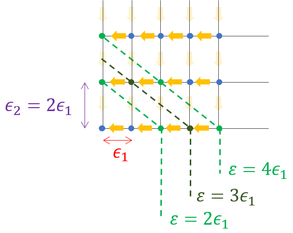
2.2 General Formulation
In more realistic situations where the different vibrational energies are not exact multiples of each other, the rate constant for emission from the thermally populated states of oscillator is still calculated by summing over the products of populations and the energy-specified rate constants. The populations are calculated with the level densities (densities of states). Let denote the density of states of total energy for which the vibrational mode is occupied times. The probability for the vibrational mode to be occupied exactly times is then . Hence the rate of decay through mode is given by:
| (4) |
which can be simplified using:
| (5) |
Here denotes the number of states of total energy where mode is occupied at least times. To prove the first equality we note that every state appears once in the sum on the left multiplied by while it is counted times in the sum on the right of this equality sign. For the equation on the right we note that once the mode is occupied at least times there remains an amount of energy to distribute within the system. Using Eq. 4 with Eq. 5 leads to:
| (6) |
The precise upper limit of the summation is indicated here with by taking the integer part of the energy in units of , . The number is the fractional part of , . The total cooling rate constant of the molecule is the sum of such contributions from each vibration:
| (7) |
The use of Eqs. 6 and Eq. 7 along with the density of states is known as the ’harmonic cascade model. Chandrasekaran et al. 2014; Bull et al. 2019
An example of the results of such a calculation is shown in Fig. 2. As with the single oscillator and the two mode examples discussed above, we observe that a general linear dependence of on , as well as fluctuations on top of the general trend. The figure also shows the effect of a variation of the width of the energy bin, , used for the calculation of the density of states. The curves for different values of agree, up to the fluctuations on top of the general trend. We need therefore not consider this issue any further.

3 Rate of Decay
In the special case where all vibrational frequencies in a molecule are identical (the Einstein molecule), simple combinatorics can be used to show that , with the common vibrational quantum energy. Trianglar brackets indicate averaging over the different vibrational modes, i.e.:
| (8) |
To treat the general case in which the vibrational levels are not degenerate, we apply the criterion of agreement of the level density with the known high energy limit. Inserting the asymptotic limit for the density of states,
| (9) |
into Eq. 6 gives
| (10) | |||||
where and . The term is asymptotically negligible compared with the first and can therefore be ignored. The sum can be approximated using Faulhaber’s formula (which are also the first two terms the Euler-Maclaurin formula):
| (11) |
Here the rightmost expression was derived using a Taylor expansion of the two powers. Inserting this approximation into Eq. 10 leads to:
| (12) |
which can be written as:
| (13) |
| (14) |
An interesting consequence is that:
| (15) |
The total decay rate is therefore given by:
| (16) |
with:
| (17) |
In particular we find that, in the asymptotic limit, has a linear dependence on internal energy . A similar scaling has previously been given in Ref. Terzieva and Herbst 2000, albeit without the offset in the linear dependence of the rate constant that will be derived here. Figure 3 shows a comparison of the calculation of the decay rate using the harmonic cascade model calculated with the Beyer-Swinehart level density, compared with the results of Eq. 16. Notably, while Eq. 16 does not account for the fluctuations on top of the general trend, it does seem to capture the general trend extremely well.

4 Population Evolution

Let denote the normalized energy distribution of a system,
| (18) |
The harmonic cascade model allows a calculation of the evolution of with time according to:
| (19) |
where the sum runs over the vibrational modes. The first term comes from states with higher energy radiatively decaying into the states of interest, and is the total rate constant for decay out of the system with energy . In this section we will find the time evolution of in terms of its mean, , and its variance: . We will analyze the high energy limit, with the understanding that this limit is a fairly good approximation to reasonably low energies, up to the fluctuation induced by the quantum discreteness (see fig. 3). In this limit the total emission rate constant is given by Eq. 16. With that expression, the energy develops as:
| (20) |
Note that upon summation the offset terms cancel out (). The energy therefore decreases exponentially:
| (21) |
The exponent in this expression is the same for all energies. Averaging over a distribution will therefore give the same decrease for the mean energy:
| (22) |
The time evolution of the variance of , , is governed by the equation
| (23) |
The last term is zero by definition of the mean value. The first term requires the time evolution of , according to Eq.19. This gives:
| (24) |
or, exchanging integration and summation,
| (25) |
The rate constants are represented with the two (known) parameters as
| (26) |
Each term in the sum can then be written as
| (27) | |||||
The first and the second terms on the right hand side cancel. Collecting terms from the remaining two integrals gives
| (28) | |||||
Inserting the values of and gives
| (29) |
Summation over all modes gives
| (30) |
or
| (31) |
This has the solution
| (32) | |||||
For the special case where all are identical, the equation reduces to
| (33) |
At long times the ratio of the standard deviation to the mean value for this case approaches the value
| (34) |
Hence the relative widths of these distributions increase as the particle cools.
Another point worth considering is if the width can increase in absolute terms. This will happen if the initial distribution is sufficiently narrow. Taking the derivative at zero time shows that the condition for this is
| (35) |
For an ensemble with an initially canonical distribution and thermally activated vibrational degrees of freedom, the value of is . This translates into the condition
| (36) |
This is a very small width and is rarely of interest in realistic situations.
It is of interest to compare the results for the mean and variances with those that describe an emission with a continuum spectrum. These cases were treated in Stenfalk and Hansen 2007 with a photon absorption cross section proportional to the photon energy to the power . Both the mean energy and the width varies asymptotically as a power law with the power , i.e. in parallel, in contrast to the exponential and non-parallel variations found here.
5 Discussion and Summary
The dynamics of vibrational cooling in the rapid exchange model has been analyzed, showing that the cooling rate has a linear dependence on internal energy. This implies that if one observes experimentally a deviation from the linear behavior, this means that the assumption of rapid IVR would be incorrect. D. Muell Furthermore, the consequences regarding the temporal evolution of the means and the variances of energy distributions that are cooled by vibrational transitions have been studied.
The main result is an exponential decrease of the mean energy with time. The time dependence of the width of the energy distribution involves several terms but will asymptotically approach an exponentially decreasing value, albeit with a time constant of twice of the one for the mean value. Distributions will therefore tend to broaden relative to the mean with time.
The high energy results fail at excitation energies around one quantum per mode and less. This is not surprising and is also clear from inspection of the literature results on C Goto et al. 2013. The energy distributions for this cluster decrease with a power of time, with the same power for width and mean. Simulated data reproduce these features with measured/calculated low energy and ground state properties, and the differences to the present results are therefore not due to new physics, but rather a consequence of the low energy limit. In lieu of a closed form expression for the photon emission rate constants rate in this limit, the equations 6, and 19 can be used to calculate the temporal development of energy distributions.
References
- Herbst and Dishoeck (2009) Herbst, E.; Dishoeck, E. F. V. Complex organic interstellar molecules. Ann. Rev. Astron. Astr. 2009, 47, 427–480.
- McGuire (2018) McGuire, B. A. 2018 Census of Interstellar, Circumstellar, Extragalactic, Protoplanetary Disk, and Exoplanetary Molecules. Astrophys. J. Suppl. S. 2018, 239, 17.
- Lange et al. (2012) Lange, M.; Froese, M. W.; Menk, S.; Bing, D.; Fellenberger, F.; Grieser, M.; Laux, F.; Orlov, D. A.; Repnow, R.; Sieber, T.; Toker, Y.; von Hahn, R.; Wolf, A.; Blaum, K. Radiative cooling of and in a cryogenic environment. New J. Phys. 2012, 14, 065007.
- Najafian et al. (2014) Najafian, K.; Pettersson, M. S.; Dynefors, B.; Shiromaru, H.; Matsumoto, J.; Tanuma, H.; Furukawa, T.; Azuma, T.; Hansen, K. Radiative cooling of . J. Chem. Phys. 2014, 140, 104311.
- Breitenfeldt et al. (2018) Breitenfeldt, C.; Blaum, K.; George, S.; Göck, J.; Guzmán-Ramírez, G.; Karthein, J.; Kolling, T.; Lange, M.; Menk, S.; Meyer, C.; Mohrbach, J.; Niedner-Schatteburg, G.; Schwalm, D.; Schweikhard, L.; Wolf, A. Long-Term Monitoring of the Internal Energy Distribution of Isolated Cluster Systems. Phys. Rev. Lett. 2018, 120, 253001.
- Bull et al. (2019) Bull, J. N.; Scholz, M. S.; Carrascosa, E.; Kristiansson, M. K.; Eklund, G.; Punnakayathil, N.; de Ruette, N.; Zettergren, H.; Schmidt, H. T.; Cederquist, H.; Stockett, M. H. Ultraslow radiative cooling of Cn- (n=3-5). J. Chem. Phys. 2019, 151, 114304.
- Stockett et al. (2020) Stockett, M.; Bull, J. N.; Buntine, J. T.; Carrascosa, E.; Anderson, E. K.; Gatchell, M.; Kaminska, M.; Nascimento, R. F.; Cederquist, H.; T., S. H.; Zettergren, H. Radiative cooling of carbon cluster anions C (). Eur. Phys. J. D 2020, 74, 150.
- Stockett et al. (2020) Stockett, M. H.; Bull, J. N.; Buntine, J. T.; Carrascosa, E.; Ji, M.; Kono, N.; Schmidt, H. T.; Zettergren, H. Unimolecular fragmentation and radiative cooling of isolated PAH ions: A quantitative study. J. Chem. Phys. 2020, 153, 154303.
- Goto et al. (2013) Goto, M.; Sundén, A.; Shiromaru, H.; Matsumoto, J.; Tanuma, H.; Azuma, T.; Hansen, K. Direct observation of internal energy distributions of C. J. Chem. Phys. 2013, 139, 054306.
- Ferrari et al. (2019) Ferrari, P.; Janssens, E.; Lievens, P.; Hansen, K. Radiative cooling of size-selected gas phase clusters. Int. Rev. Phys. Chem. 2019, 38, 405.
- Iida et al. (2021) Iida, S.; Kuma, S.; Kuriyama, M.; Furukawa, T.; Kusunoki, M.; Tanuma, H.; Hansen, K.; Shiromaru, H.; Azuma, T. IR-photon quenching of delayed electron detachment from hot pentacene anions. Phys. Rev. A 2021, 104, 043114.
- (12) D. Muell, Y. T. e. a., H. Kreckel In preparation: Radiative cooling of Al and Al in a cryogenic environment.
- Bixon and Jortner (1968) Bixon, M.; Jortner, J. Intramolecular Radiationless Transitions. J. Chem. Phys. 1968, 48, 715.
- Gruebele and Wolynes (2004) Gruebele, M.; Wolynes, P. G. Vibrational Energy Flow and Chemical Reactions. Acc. Chem. Res. 2004, 37, 261–267.
- Makarov et al. (2012) Makarov, A. A.; Malinovsky, A. L.; Ryabov, E. A. Intramolecular vibrational redistribution: from high-resolution spectra to real-time dynamics. Uspekhi Fizicheskih Nauk 2012, 182, 977.
- Nesbitt and Field (1996) Nesbitt, D. J.; Field, R. W. Vibrational Energy Flow in Highly Excited Molecules: Role of Intramolecular Vibrational Redistribution. J. Phys. Chem. 1996, 100, 12735–12756.
- Hansen and Ferrari (2021) Hansen, K.; Ferrari, P. Vibrational angular momentum level densities of linear molecules. Chem. Phys. Lett. 2021, 768, 138385.
- Brink and Stringari (1990) Brink, D. M.; Stringari, S. Density of states and evaporation rate of helium clusters. Z Phys D 1990, 15, 257–263.
- Lehmann (2004) Lehmann, K. K. Bias in the temperature of helium nanodroplets measured by an embedded rotor. J. Chem. Phys. 2004, 120, 513.
- Hansen et al. (2007) Hansen, K.; Johnson, M. D.; Kresin, V. V. Density of states of helium droplets. Phys. Rev. B 2007, 76, 235424.
- Chandrasekaran et al. (2014) Chandrasekaran, V.; Kafle, B.; Prabhakaran, A.; Heber, O.; Rappaport, M.; Rubinstein, H.; Schwalm, D.; Toker, Y.; Zajfman, D. Determination of Absolute Recurrent Fluorescence Rate Coefficients for C6–. J. Phys. Chem. Lett. 2014, 5, 4078–4082.
- Terzieva and Herbst (2000) Terzieva, R.; Herbst, E. Radiative electron attachment to small linear carbon clusters and its significance for the chemistry of diffuse interstellar clouds. Int. J. Mass Spetrom. 2000, 201, 135–142.
- Stenfalk and Hansen (2007) Stenfalk, J.; Hansen, K. Energy distributions of clusters cooled by thermal radiation. Eur. Phys. J. D 2007, 43, 101.