跳到论文正文
W Papers独立论文阅读器 arXiv:2211.13541 论文正文 计算阅读时间 · 0%
引用这篇论文根据当前论文元数据生成,正式投稿前建议核对。


License: CC BY 4.0
arXiv:2211.13541v2 [eess.IV] 28 Jul 2023

A mathematical theory of resolution limits for super-resolution of positive sources Thanks: This work was supported in part by the Swiss National Science Foundation grant number 200021–200307.

Ping Liu Thanks: Department of Mathematics, ETH Zürich, Rämistrasse 101, CH-8092 Zürich, Switzerland (ping.liu@sam.math.ethz.ch, yanchen.he@sam.math.ethz.ch, habib.ammari@math.ethz.ch).    Yanchen He22footnotemark: 2    Habib Ammari22footnotemark: 2
Abstract

A priori information on the positivity of source intensities is ubiquitous in imaging fields, and is also important for a multitude of super-resolution and deconvolution algorithms. But the fundamental resolution limit of positive sources is still unknown, and research in this field is very limited indeed. In this work, we analyze the super-resolving capacity for number and location recoveries in the super-resolution of positive sources and aim to answer the resolution limit problem in a rigorous manner. Specifically, we introduce the computational resolution limit for respectively the number detection and location recovery in the one-dimensional super-resolution problem and quantitatively characterize their dependency on the cutoff frequency, signal-to-noise ratio, and the sparsity of the sources. As a direct consequence, we show that targeting at the sparest positive solution in the super-resolution already provides the optimal resolution order. These results are generalized to multi-dimensional spaces. Our estimates indicate that there exist phase transitions in the corresponding reconstructions, which are confirmed by numerical experiments. On the other hand, despite the fact that positivity plays important roles in improving the resolution of certain super-resolution algorithms, our theory has made several different but significant discoveries: i) The a priori information of positivity cannot further improve the order of the resolution limit; ii) The positivity of the source sometimes deteriorates the resolution limit instead of enhancing it. In particular, under certain the signal-to-noise ratio, two point sources with different phases actually have better resolution limit than those with the same one.

Mathematics Subject Classification: 65R32, 42A10, 15A09, 94A08, 94A12

Keywords: resolution limit, super-resolution, positive sources, line spectral estimation, Vandermonde matrix, phase transition

1 Introduction

In recent years, the development of super-resolution optical microscopy led to a revolutionary improvement of resolution through the use of different technical approaches. This impressive success has generated significant interest in studying the super-resolution algorithms and the fundamental super-resolving capability. In this paper, we aim to study the super-resolving capacity of the number and locations recovery in the super-resolution of positive sources. To be more specific, we consider the following mathematical model. Let μ=∑j=1naj​δyj,aj>0\mu=\sum_{j=1}^{n}a_{j}\delta_{y_{j}},a_{j}>0 be a positive discrete measure, where yj∈ℝ,j=1,⋯,ny_{j}\in\mathbb{R},j=1,\cdots,n, represent the location of the point sources and aj>0,j=1,⋯,n,a_{j}>0,j=1,\cdots,n, their amplitudes. Noting that yjy_{j}’s are the supports of the Dirac masses in μ\mu. In this paper we will use support recovery instead of location reconstruction. We denote by

mmin=minj=1,⋯,n⁡aj,dmin=minp≠j⁡|yp−yj|.m_{\min}=\min_{j=1,\cdots,n}a_{j},\quad d_{\min}=\min_{p\neq j}|y_{p}-y_{j}|.

The measurement is the noisy Fourier data of μ\mu in a bounded interval, that is,

𝐘⁡(ω)=ℱ⁡[μ]​(ω)+𝐖⁡(ω)=∑j=1naj​ei​yj​ω+𝐖⁡(ω),ω∈[−Ω,Ω],\mathbf{Y}(\omega)=\mathcal{F}[\mu](\omega)+\mathbf{W}(\omega)=\sum_{j=1}^{n}a_{j}e^{iy_{j}\omega}+\mathbf{W}(\omega),\quad\omega\in[-\Omega,\Omega], (1.1)

with 𝐖⁡(ω)\mathbf{W}(\omega) being the noise and Ω\Omega the cutoff frequency of the imaging system. We assume that

|𝐖⁡(ω)|<σ,ω∈[−Ω,Ω],|\mathbf{W}(\omega)|<\sigma,\quad\omega\in[-\Omega,\Omega],

with σ\sigma being the noise level. The above measurement model is chosen for convenience. All the results in this paper also hold for the case when taking measurement at a sufficient number of evenly-spaced points as what was considered in [31]. Thus our results can be applied to practical situations and real-world problems.

The super-resolution problem we are interested in is to recover the positive discrete measure μ\mu from the above noisy measurement 𝐘\mathbf{Y}. We note that the super-resolution problem is closely related to the line spectral estimation problem [31] which is at the core of diverse fields such as wireless communications and array processing. It should also be pointed out that the measurement discussed in equation (1.1) pertains to imaging the convolution of positive point sources with a band-limited or general point spread function ff. Therefore, with slight modifications, our findings can also be employed to analyze the stability of deconvolving positive sources, which is a crucial problem in various fields.

1.1 Literature review

Fundamental limits. In [42, 43, 21], the authors analyzed the resolution limit in the detection of two closely-spaced point sources based on the statistical inference theory, but their theory has not been generalized to the case when there are more than two sources in the signal. The mathematical theory for analyzing the fundamental limit in super-resolving multiple point sources was pioneered by Donoho [14] in 1992. In that work, he considered a grid setting where a discrete measure is supported on a lattice with spacing Δ\Delta and regularized by a so-called "Rayleigh index". The problem is to reconstruct the amplitudes of the grid points from their noisy Fourier data in [−Ω,Ω][-\Omega,\Omega] with Ω\Omega being the band limit. His main contribution is estimating the corresponding minimax error in the recovery, which emphasizes the importance of the sparsity of sources for the super-resolution. It was improved in recent years for the case when only nn point sources are presented. In [12], the authors considered resolving nn-sparse point sources supported on a grid and showed that the minimax error of amplitude recovery in the presence of noise with magnitude σ\sigma scales exactly as S​R​F2​n−1​σSRF^{2n-1}\sigma, where S​R​F:=1Δ​ΩSRF:=\frac{1}{\Delta\Omega} is the super-resolution factor. The case of multi-clustered point sources was considered in [24, 4] and similar minimax error estimates were derived. Moreover, in [2, 5] the authors considered the minimax error for recovering the amplitudes and locations of off-the-grid point sources. They showed that for σ⪅(S​R​F)−2​p+1\sigma\lessapprox(SRF)^{-2p+1}, where pp is the number of point sources in a cluster, the minimax error for the amplitude and the location recoveries scale respectively as (S​R​F)2​p−1​σ(SRF)^{2p-1}\sigma, (S​R​F)2​p−2​σ/Ω(SRF)^{2p-2}{\sigma}/{\Omega}, while for the single non-clustered source away from other sources, the corresponding minimax error for the amplitude and the location recoveries scale respectively as σ\sigma and σ/Ω{\sigma}/{\Omega}. We also refer the readers to [33, 8] for understanding the resolution limit from the perspective of sample complexity and to [47, 11] for the resolving limit of some algorithms.

On the other hand, in order to characterize the exact resolution in resolving multiple point sources like the classical Rayleigh limit, in the earlier works [32, 30, 31, 29, 27] we defined the concept of "computational resolution limit" as the minimum required distance between point sources so that their number and locations can be stably resolved under certain noise level. By developing a non-linear approximation theory in a so-called Vandermonde space, we derived sharp bounds for computational resolution limits in one- and multi-dimensional super-resolution problems. In particular, we showed that the computational resolution limits for number and location recoveries should be respectively Cnum​(n,k)Ω​(σmmin)12​n−2\frac{C_{\mathrm{num}}(n,k)}{\Omega}\left(\frac{\sigma}{m_{\min}}\right)^{\frac{1}{2n-2}} and Csupp​(n,k)Ω​(σmmin)12​n−1\frac{C_{\mathrm{supp}}(n,k)}{\Omega}\left(\frac{\sigma}{m_{\min}}\right)^{\frac{1}{2n-1}}, where Cnum​(n,k),Csupp​(n,k)C_{\mathrm{num}}(n,k),C_{\mathrm{supp}}(n,k) are constants depending only on source number nn and space dimensionality kk. In this paper, we will generalize these results to the super-resolution problem of positive sources.

Reconstruction algorithms. Due to the importance of super-resolution in applications, a number of sophisticated super-resolution algorithms have been developed over the years. Among those algorithms, a class of algorithms called subspace methods have exhibited favourable performance and have been used frequently in engineering applications. Specific examples include MUltiple SIgnal Classification (MUSIC) [40], Estimation of Signal Parameters via Rotational Invariance Technique (ESPRIT) [39], and Matrix Pencil Method [22]. Note that these algorithms date back to the work of Prony [37]. Despite the appealing performance of the subspace methods in practical applications, their stability properties are not yet well-understood. The asymptotic results on the stability of MUSIC algorithm in the presence of Gaussian noise were derived just slightly after its emerging [45, 9, 46]. But only until recent years, some steps towards understanding the stability of MUSIC, ESPRIT and Matrix-Pencil Method in the non-asymptotic regime were taken in [26], [25] and [33], respectively. Nevertheless, the error tolerance derived in these papers are not as strong as our estimates here for the resolution limit in location reconstruction. On the other hand, it was shown numerically in [26, 5, 25] that these subspace methods actually achieve the optimal resolution order. Thus the theoretical demonstrations for the performance limits of subspace methods in the non-asymptotic regime are still important open problems.

In recent years, inspired by the idea of sparse modeling and compressed sensing, many sparsity promoting algorithms have been proposed for the super-resolution problem. For example, in the groundbreaking work of Candès and Fernandez-Granda [7], it was proved that off-the-grid sources can be exactly recovered from their low-frequency measurements by a TV minimization under a minimum separation condition. It invokes active researches in the off-the-grid algorithms, among them we would like to mention the BLASSO [3, 16, 36] and the atomic norm minimization method [49, 48]. Both methods were proved to be able to stably recover the source under a minimum separation condition or a non-degeneracy condition.

Super-resolution of positive sources. To the best of our knowledge, the theoretical possibility for the super-resolution of positive sources was first considered in [15]. Specifically, the authors defined

ω⁡(σ,𝐱)=sup{‖𝐱′−𝐱‖1:‖K​𝐱′−K​𝐱‖2⩽σ​ and ​𝐱′⩾0},\omega(\sigma;\mathbf{x})=\sup\left\{\left\|\mathbf{x}^{\prime}-\mathbf{x}\right\|_{1}:\left\|K\mathbf{x}^{\prime}-K\mathbf{x}\right\|_{2}\leqslant\sigma\text{ and }\mathbf{x}^{\prime}\geqslant 0\right\},

where 𝐱,𝐱′\boldsymbol{\mathbf{x}},\boldsymbol{\mathbf{x}}^{\prime} are vectors of length MM (sources are on a grid) and KK consists of the first mm rows of the M×MM\times M discrete Fourier transform, and said that 𝐱\mathbf{x} admits super-resolution if

ω⁡(σ,𝐱)→0 as ​σ→0.\omega(\sigma;\mathbf{x})\rightarrow 0\quad\text{ as }\sigma\rightarrow 0.

They demonstrated for 𝐱≥0\boldsymbol{\mathbf{x}}\geq 0 that: (a) If 𝐱\mathbf{x} has 12​(m−1)\frac{1}{2}(m-1) or fewer non-zero elements then 𝐱\boldsymbol{\mathbf{x}} admits super-resolution; (b) If 12​(m+1)\frac{1}{2}(m+1) divides MM, there exists 𝐱\mathbf{x} with 12​(m+1)\frac{1}{2}(m+1) non-zero elements yet does not admit super-resolution; (c) If 𝐱\mathbf{x} has more than mm non-zero elements then 𝐱\boldsymbol{\mathbf{x}} does not admit super-resolution. Their definition and results focused on the possibility of overcoming Rayleigh limit in the presence of sufficient small noise and hence demonstrated the possibility of super-resolution. See also [18] for a shorter exposition of the same idea.

In recent years, some researchers analyzed the stability of specific super-resolution algorithms in a non-asymptotic regime [35, 34, 13]. To be more specific, it was shown in [35] that a simple convex optimization program can already superresolve the positive sources (on a grid) to nearly optimal. The authors of [35] demonstrated that under certain conditions the deviation between the algorithm’s output 𝐱^\hat{\mathbf{x}} and the ground truth 𝐱\mathbf{x} obeys the following relation

‖𝐱^−𝐱‖1≈C⋅SRF2​r⋅σ,\|\hat{\mathbf{x}}-\mathbf{x}\|_{1}\approx C\cdot\mathrm{SRF}^{2r}\cdot\sigma,

where rr is the Rayleigh index. The theory was later generalized to the off-the-grid setting in [34] where the authors analyzed the stability of the reconstruction of high frequency information. In a different line of research, the authors studied in [13] the amplitude and support recoveries of positive discrete measures for a so-called BLASSO convex program. They demonstrated that when σ/λ,σ/dmin2​n−1\sigma/\lambda,\sigma/d_{\min}^{2n-1} and λ/dmin2​n−1\lambda/d_{\min}^{2n-1} are sufficiently small (with λ\lambda being the regularization parameter, σ\sigma the noise level, nn the source number, dmind_{\min} the minimum separation distance between two sources), there exists a unique solution to the BLASSO program consisting of exactly nn point sources. The amplitudes and locations of the solution both converge toward those of the ground truth when the noise and the regularization parameter decay to zero faster than dmin2​n−1d_{\min}^{2n-1}. Note that this result is consistent with our estimates in the current paper, showing that the BLASSO achieves the optimal resolution order, which is quite impressive. We also refer the readers to many other algorithms [6, 17, 23, 19, 10] leveraging the a priori knowledge of positivity and especially the well-known maximum entropy method [20, 15].

1.2 Main contribution

The main contribution of this paper is quantitative characterizations of the resolution limits to number detection and location recovery in the super-resolution of positive sources. Accurate detection of the source number (model order) is important in the super-resolution problem and many parametric estimation methods require the model order as a priori information. But there are few theoretical results which address the issue when the number of underlying sources is greater than two. In [32, 31], the first results for capacity of the number detection in the super-resolution of general sources are derived. Here we generalize the estimates to the case of positive sources, which is also the first result for understanding the capacity of super-resolving positive sources. Specifically, we introduce the computational resolution limit 𝒟n​u​m+\mathcal{D}_{num}^{+} for the detection of nn point sources (see Definition 2.2), and derive the following sharp bounds:

2​e−1Ω​(σmmin)12​n−2<𝒟n​u​m+≤2​e​πΩ​(σmmin)12​n−2,\frac{2e^{-1}}{\Omega}\Big(\frac{\sigma}{m_{\min}}\Big)^{\frac{1}{2n-2}}<\mathcal{D}_{num}^{+}\leq\frac{2e\pi}{\Omega}\Big(\frac{\sigma}{m_{\min}}\Big)^{\frac{1}{2n-2}}, (1.2)

where σmmin\frac{\sigma}{m_{\min}} is viewed as the inverse of the signal-to-noise ration (SNR). It follows that exact detection of the source number is possible when the minimum separation distance of point sources dmind_{\min} is greater than 2​e​πΩ​(σmmin)12​n−2\frac{2e\pi}{\Omega}\Big(\frac{\sigma}{m_{\min}}\Big)^{\frac{1}{2n-2}}, and impossible without additional a priori information when dmind_{\min} is less than 2​e−1Ω​(σmmin)12​n−2\frac{2e^{-1}}{\Omega}\Big(\frac{\sigma}{m_{\min}}\Big)^{\frac{1}{2n-2}} in the worst-case scenario.

Following the same line of argument for the number detection problem, we also consider the location recovery in the super-resolution of positive sources. We introduce the computational resolution limit 𝒟s​u​p​p+\mathcal{D}_{supp}^{+} for the support recovery (see Definition 2.4) and derive the following bounds:

2​e−1Ω​(σmmin)12​n−1<𝒟s​u​p​p+≤2.36​e​πΩ​(σmmin)12​n−1.\frac{2e^{-1}}{\Omega}\Big(\frac{\sigma}{m_{\min}}\Big)^{\frac{1}{2n-1}}<\mathcal{D}_{supp}^{+}\leq\frac{2.36e\pi}{\Omega}\Big(\frac{\sigma}{m_{\min}}\Big)^{\frac{1}{2n-1}}. (1.3)

As a consequence, the resolution limit 𝒟s​u​p​p+\mathcal{D}_{supp}^{+} is of the order O⁡(1Ω​(σmmin)12​n−1)O(\frac{1}{\Omega}\Big(\frac{\sigma}{m_{\min}}\Big)^{\frac{1}{2n-1}}). It follows that stable recovery (in certain sense) of the source locations is possible when the minimum separation distance of point sources dmind_{\min} is greater than 2.36​e​πΩ​(σmmin)12​n−1\frac{2.36e\pi}{\Omega}\Big(\frac{\sigma}{m_{\min}}\Big)^{\frac{1}{2n-1}}, and impossible without additional a priori information when dmind_{\min} is less than 2​e−1Ω​(σmmin)12​n−1\frac{2e^{-1}}{\Omega}\Big(\frac{\sigma}{m_{\min}}\Big)^{\frac{1}{2n-1}} in the worst-case scenario. To further emphasize that the separation distance O⁡(1Ω​(σmmin)12​n−1)O\left(\frac{1}{\Omega}\Big(\frac{\sigma}{m_{\min}}\Big)^{\frac{1}{2n-1}}\right) is necessary for a stable location reconstruction, we construct an example showing that if the sources are separated below the cΩ​(σmmin)12​n−1\frac{c}{\Omega}\Big(\frac{\sigma}{m_{\min}}\Big)^{\frac{1}{2n-1}} for certain constant cc, the recovered locations can be very unstable.

As a direct consequence of our estimates, we analyze the stability for a sparsity-promoting algorithm (l0l_{0} minimization) in super-resolving positive sources and show that it already achieves the optimal order of the resolution. These estimates for the resolution limits are also generalized to multi-dimensional spaces.

The quantitative characterizations of the resolution limits 𝒟n​u​m+\mathcal{D}_{num}^{+} and 𝒟s​u​p​p+\mathcal{D}_{supp}^{+} imply phase transition phenomena in the corresponding reconstructions, which are confirmed here by numerical experiments.

In addition, our results reveal that a priori knowledge of the positivity of the source does not improve the resolution limit order compared to resolving complex sources [31, 28]. The question of whether positivity can indeed enhance the resolution limit arises. The answer is no. Specifically, we demonstrate that under certain noise level, the computational resolution limit for distinguishing two sources (number detection) with a phase difference θ\theta (in amplitude) is

𝒟k,n​u​m=4​arcsin⁡((σmmin)12)−θΩ.\mathcal{D}_{k,num}=\frac{4\arcsin\left(\left(\frac{\sigma}{m_{\min}}\right)^{\frac{1}{2}}\right)-\theta}{\Omega}.

This shows that the positivity of two sources actually deteriorates the resolution limit rather than enhancing it. As another discovery, we see that achieving super-resolution in distinguishing images generated from one or two sources is quite possible, especially when the source amplitudes differ in phases.

On the other hand, our techniques offer a way to analyze the capability of resolving positive sources, which could inspire future work.

1.3 Organization of the paper

The paper is organized in the following way. Section 2 presents the estimates for the resolution limit in the one-dimensional super-resolution of positive sources. Section 3 extends the estimates to multi-dimensional spaces. In Section 4, we discuss if the positivity can indeed enhance the resolution limit. In Sections 5 and 6, we verify the phase transition in respectively the number detection and location recovery problems. The purpose of Section 7 is to make a few final remarks. Section 8 and Section 9 prove respectively the results in Section 2 and Section 4. In Appendix A, we prove several auxiliary lemmas and useful inequalities.

2 Resolution limits for super-resolution in one-dimensional space

We present in this section our main results on the resolution limit for the super-resolution of one-dimensional positive sources. All the results shall be proved in Section 8. We consider the case when the point sources are tightly spaced and form a cluster. To be more specific, we define the interval

I(n,Ω):=(−(n−1)​π2​Ω,(n−1)​π2​Ω),I(n,\Omega):=\Big(-\frac{(n-1)\pi}{2\Omega},\quad\frac{(n-1)\pi}{2\Omega}\Big),

which is of length of several Rayleigh limits and assume that yj∈I⁡(n,Ω),1≤j≤ny_{j}\in I(n,\Omega),1\leq j\leq n. The reconstruction process is usually targeting at some specific solutions in a so-called admissible set, which comprises of discrete measures whose Fourier data are sufficiently close to 𝐘\boldsymbol{\mathbf{Y}}. In our problem, we introduce the following concept of positive σ\sigma-admissible discrete measures. We denote in this section ||f||∞=maxω∈[−Ω,Ω]⁡|f⁡(ω)|\left|\left|{f}\right|\right|_{\infty}=\max_{\omega\in[-\Omega,\Omega]}|f(\omega)|.

Definition 2.1.

Given measurement 𝐘\mathbf{Y}, we say that μ^=∑j=1ka^j​δy^j,a^j>0\hat{\mu}=\sum_{j=1}^{k}\hat{a}_{j}\delta_{\hat{y}_{j}},\hat{a}_{j}>0 is a positive σ\sigma-admissible discrete measure of 𝐘\ \mathbf{Y} if

||ℱ⁡[μ^]−𝐘||∞<σ.\left|\left|{\mathcal{F}[\hat{\mu}]-\mathbf{Y}}\right|\right|_{\infty}<\sigma.

The set of positive σ\sigma-admissible measures of 𝐘\mathbf{Y} characterizes all possible solutions to our super-resolution problem with the given measurement 𝐘\mathbf{Y}. Following similar definitions in [31, 32, 30, 28], we define the following computational resolution limit for the number detection in the super-resolution of positive sources. The reason for the definition is the fact that detecting the correct source number in μ\mu is impossible without additional a prior information when there exists one positive σ\sigma-admissible measure with less than nn supports.

Definition 2.2.

The computational resolution limit to the number detection problem in the super-resolution of one-dimensional positive source is defined as the smallest nonnegative number 𝒟n​u​m+\mathcal{D}_{num}^{+} such that for all positive nn-sparse measure ∑j=1naj​δyj,aj>0,yj∈I⁡(n,Ω)\sum_{j=1}^{n}a_{j}\delta_{y_{j}},a_{j}>0,y_{j}\in I(n,\Omega) and the associated measurement 𝐘\boldsymbol{\mathbf{Y}} in (1.1), if

minp≠j⁡|yj−yp|≥𝒟n​u​m+,\min_{p\neq j}|y_{j}-y_{p}|\geq\mathcal{D}_{num}^{+},

then there does not exist any positive σ\sigma-admissible measure of 𝐘\ \mathbf{Y} with less than nn supports.

The notion of “computational resolution limit” emphasizes the essential impossibility of correct number detection for very close source by any means. Also, this notion depends crucially on the signal-to-noise ratio and the sparsity of the source, which is different from all classical resolution limits [1, 50, 38, 41, 44] that depend only on the cutoff frequency. We now present sharp bounds for this computational resolution limit 𝒟n​u​m+\mathcal{D}_{num}^{+}. The following upper bound for it is a direct consequence of [28, Theorem 3.1].

Theorem 2.1.

Let 𝐘\mathbf{Y} be a measurement generated by a positive measure μ=∑j=1naj​δyj\mu=\sum_{j=1}^{n}a_{j}\delta_{y_{j}}, which is supported on I⁡(n,Ω)I(n,\Omega). Let n≥2n\geq 2 and assume that the following separation condition is satisfied

minp≠j⁡|yp−yj|≥2​e​πΩ​(σmmin)12​n−2.\min_{p\neq j}\Big|y_{p}-y_{j}\Big|\geq\frac{2e\pi}{\Omega}\Big(\frac{\sigma}{m_{\min}}\Big)^{\frac{1}{2n-2}}. (2.1)

Then there do not exist any positive σ\sigma-admissible measures of  𝐘\mathbf{Y} with less than nn supports.

Theorem 2.1 gives an upper bound for the computational resolution limit 𝒟n​u​m+\mathcal{D}_{num}^{+}. This upper bound is shown to be tight for the super-resolution of general discrete source (not positive) by a lower bound derived in [31], but the result is unknown for the case of resolving positive sources. We next present a lower bound of 𝒟n​u​m+\mathcal{D}_{num}^{+} which is the main result of this paper.

Theorem 2.2.

For given 0<σ≤mmin0<\sigma\leq m_{\min} and integer n≥2n\geq 2, there exist positive measures μ=∑j=1naj​δyj\mu=\sum_{j=1}^{n}a_{j}\delta_{y_{j}} with nn supports and μ^=∑j=1n−1a^j​δy^j\hat{\mu}=\sum_{j=1}^{n-1}\hat{a}_{j}\delta_{\hat{y}_{j}} with (n−1)(n-1) supports such that ||ℱ⁡[μ^]−ℱ⁡[μ]||∞<σ\left|\left|{\mathcal{F}[\hat{\mu}]-\mathcal{F}[\mu]}\right|\right|_{\infty}<\sigma. Moreover,

min1≤j≤n⁡|aj|=mmin,minp≠j⁡|yp−yj|=2​e−1Ω​(σmmin)12​n−2.\min_{1\leq j\leq n}\left|{a_{j}}\right|=m_{\min},\quad\min_{p\neq j}\left|{y_{p}-y_{j}}\right|=\frac{2e^{-1}}{\Omega}\Big(\frac{\sigma}{m_{\min}}\Big)^{\frac{1}{2n-2}}.

The above result gives a lower bound for the computational resolution limit 𝒟n​u​m+\mathcal{D}_{num}^{+} to the number detection problem. Combined with Theorem 2.1, it reveals that the computational resolution limit for number detection satisfies

2​e−1Ω​(σmmin)12​n−2<𝒟n​u​m+≤2​e​πΩ​(σmmin)12​n−2.\frac{2e^{-1}}{\Omega}\Big(\frac{\sigma}{m_{\min}}\Big)^{\frac{1}{2n-2}}<\mathcal{D}_{num}^{+}\leq\frac{2e\pi}{\Omega}\Big(\frac{\sigma}{m_{\min}}\Big)^{\frac{1}{2n-2}}.

We remark that similar to the results of [2, 5, 31], our bounds are the worst-case bounds, and one may achieve better bounds for the case of random noise.

We now consider the location (support) recovery problem in the super-resolution of positive sources. We first introduce the following concept of δ\delta-neighborhood of a discrete measure.

Definition 2.3.

Let μ=∑j=1naj​δyj\mu=\sum_{j=1}^{n}a_{j}\delta_{y_{j}} be a discrete measure and let 0<δ0<\delta be such that the nn intervals (yk−δ,yk+δ),1≤k≤n(y_{k}-\delta,y_{k}+\delta),1\leq k\leq n are pairwise disjoint. We say that μ^=∑j=1na^j​δy^j\hat{\mu}=\sum_{j=1}^{n}\hat{a}_{j}\delta_{\hat{y}_{j}} is within δ\delta-neighborhood of μ\mu if each y^j\hat{y}_{j} is contained in one and only one of the n intervals (yk−δ,yk+δ),1≤k≤n(y_{k}-\delta,y_{k}+\delta),1\leq k\leq n.

According to the above definition, a measure in a δ\delta-neighbourhood preserves the inner structure of the real source. For any stable support recovery algorithm, the output should be a measure in some δ\delta-neighborhood, otherwise it is impossible to distinguish which is the reconstructed location of some yjy_{j}’s. We now introduce the computational resolution limit for stable support recoveries. For ease of exposition, we only consider measures supported in I⁡(n,Ω)I(n,\Omega), where nn is the number of supports.

Definition 2.4.

The computational resolution limit to the stable support recovery problem in the super-resolution of one-dimensional positive sources is defined as the smallest nonnegative number 𝒟s​u​p​p+\mathcal{D}_{supp}^{+} such that for all positive nn-sparse measures ∑j=1naj​δyj,aj>0,yj∈I⁡(n,Ω)\sum_{j=1}^{n}a_{j}\delta_{y_{j}},a_{j}>0,y_{j}\in I(n,\Omega) and the associated measurement 𝐘\boldsymbol{\mathbf{Y}} in (1.1), if

minp≠j⁡|yj−yp|≥𝒟s​u​p​p+,\min_{p\neq j}|y_{j}-y_{p}|\geq\mathcal{D}_{supp}^{+},

then there exists δ>0\delta>0 such that any positive σ\sigma-admissible measure for 𝐘\mathbf{Y} with nn supports in I⁡(n,Ω)I(n,\Omega) is within a δ\delta-neighbourhood of μ\mu.

To state the results on the resolution limit to stable support recovery, we introduce the super-resolution factor which is defined as the ratio between Rayleigh limit πΩ\frac{\pi}{\Omega} (for point spread function s​i​n​c​(x)2sinc(x)^{2}) and the minimum separation distance of sources dmin:=minp≠j⁡|yp−yj|d_{\min}:=\min_{p\neq j}|y_{p}-y_{j}|:

S​R​F:=πΩ​dmin.SRF:=\frac{\pi}{\Omega d_{\min}}.

As a direct consequence of [28, Theorem 3.2], we have the following theorem giving the upper bound of 𝒟s​u​p​p+\mathcal{D}_{supp}^{+}.

Theorem 2.3.

Let n≥2n\geq 2, assume that the positive measure μ=∑j=1naj​δyj\mu=\sum_{j=1}^{n}a_{j}\delta_{y_{j}} is supported on I⁡(n,Ω)I(n,\Omega) and that

minp≠j⁡|yp−yj|≥2.36​e​πΩ​(σmmin)12​n−1.\min_{p\neq j}\left|y_{p}-y_{j}\right|\geq\frac{2.36e\pi}{\Omega}\Big(\frac{\sigma}{m_{\min}}\Big)^{\frac{1}{2n-1}}. (2.2)

If μ^=∑j=1na^j​δy^j,a^j>0\hat{\mu}=\sum_{j=1}^{n}\hat{a}_{j}\delta_{\hat{y}_{j}},\hat{a}_{j}>0 supported on I⁡(n,Ω)I(n,\Omega) is a positive σ\sigma-admissible measure for the measurement generated by μ\mu, then μ^\hat{\mu} is within the dmin2\frac{d_{\min}}{2}-neighborhood of μ\mu. Moreover, after reordering the y^j\hat{y}_{j}’s, we have

|y^j−yj|<C⁡(n)Ω​S​R​F2​n−2​σmmin,1≤j≤n,\left|\hat{y}_{j}-y_{j}\right|<\frac{C(n)}{\Omega}SRF^{2n-2}\frac{\sigma}{m_{\min}},\quad 1\leq j\leq n, (2.3)

where C⁡(n)=22​n−32​e2​n−1​(max⁡(n−2,1)​π)−12C(n)=2^{2n-\frac{3}{2}}e^{2n-1}(\max(\sqrt{n-2},1)\pi)^{-\frac{1}{2}}.

Theorem 2.3 gives an upper bound to the computational resolution limit 𝒟s​u​p​p+\mathcal{D}_{supp}^{+}. We next show that the order of the upper bound is optimal.

Theorem 2.4.

For given 0<σ≤mmin0<\sigma\leq m_{\min} and integer n≥2n\geq 2, let

τ=e−1Ω​(σmmin)12​n−1.\tau=\frac{e^{-1}}{\Omega}\ \Big(\frac{\sigma}{m_{\min}}\Big)^{\frac{1}{2n-1}}. (2.4)

Then there exist a positive measure μ=∑j=1naj​δyj\mu=\sum_{j=1}^{n}a_{j}\delta_{y_{j}} with nn supports at {−(n−12)​τ,−(n−52)​τ,⋯,(n−32)​τ}\{-(n-\frac{1}{2})\tau,-(n-\frac{5}{2})\tau,\cdots,(n-\frac{3}{2})\tau\} and a positive measure μ^=∑j=1na^j​δy^j\hat{\mu}=\sum_{j=1}^{n}\hat{a}_{j}\delta_{\hat{y}_{j}} with nn supports at {−(n−32)​τ,−(n−72)​τ,⋯,(n−12)​τ}\{-(n-\frac{3}{2})\tau,-(n-\frac{7}{2})\tau,\cdots,(n-\frac{1}{2})\tau\} such that

‖ℱ⁡[μ^]−ℱ⁡[μ]‖∞<σ,min1≤j≤n⁡|aj|=mmin.||\mathcal{F}[\hat{\mu}]-\mathcal{F}[\mu]||_{\infty}<\sigma,\quad\min_{1\leq j\leq n}|a_{j}|=m_{\min}.

Since the minimum distance between yjy_{j}’s is dmin=2​τd_{\min}=2\tau, thus for the positive σ\sigma-admissible measure μ^\hat{\mu}, it is obviously that the y^j\hat{y}_{j}’s are not in any δ\delta-neighborhood of yjy_{j}’s for δ≤dmin2\delta\leq\frac{d_{\min}}{2} (for δ>dmin2\delta>\frac{d_{\min}}{2} the intervals in Definition 2.3 are overlapped). According to Definition 2.4, Theorem 2.4 implies 𝒟s​u​p​p+>2​e−1Ω​(σmmin)12​n−1\mathcal{D}_{supp}^{+}>\frac{2e^{-1}}{\Omega}\ \Big(\frac{\sigma}{m_{\min}}\Big)^{\frac{1}{2n-1}}. Thus we conclude that

2​e−1Ω​(σmmin)12​n−1<𝒟s​u​p​p+≤2.36​e​πΩ​(σmmin)12​n−1.\frac{2e^{-1}}{\Omega}\ \Big(\frac{\sigma}{m_{\min}}\Big)^{\frac{1}{2n-1}}<\mathcal{D}_{supp}^{+}\leq\frac{2.36e\pi}{\Omega}\ \Big(\frac{\sigma}{m_{\min}}\Big)^{\frac{1}{2n-1}}.

To further demonstrate that the order O⁡(1Ω​(σmmin)12​n−1)O\left(\frac{1}{\Omega}\left(\frac{\sigma}{m_{\min}}\right)^{\frac{1}{2n-1}}\right) is essentially optimal for stable location reconstruction, we present an example with a new distribution of the source locations as follows.

Proposition 2.1.

For given 0<σ<mmin0<\sigma<m_{\min} and integer n≥2n\geq 2, let

τ=0.2​e−1Ω​s2​n+12​n−1​(σmmin)12​n−1.\tau=\frac{0.2e^{-1}}{\Omega s^{\frac{2n+1}{2n-1}}}\ \Big(\frac{\sigma}{m_{\min}}\Big)^{\frac{1}{2n-1}}. (2.5)

Then there exist a positive measure μ=∑j=1naj​δyj\mu=\sum_{j=1}^{n}a_{j}\delta_{y_{j}} with nn supports at {tj=−s​n−22​τ+(j−2)​s2​τ,j=2,4,⋯,2​n}\{t_{j}=-\frac{sn-2}{2}\tau+\frac{(j-2)s}{2}\tau,j=2,4,\cdots,2n\} and a positive measure μ^=∑j=1na^j​δy^j\hat{\mu}=\sum_{j=1}^{n}\hat{a}_{j}\delta_{\hat{y}_{j}} with nn supports at {tj=t4​⌈j+14⌉−2+(−1)j+12​τ,j=1,3,5,⋯,2​n−1}\{t_{j}=t_{4\lceil\frac{j+1}{4}\rceil-2}+(-1)^{\frac{j+1}{2}}\tau,j=1,3,5,\cdots,2n-1\} such that

‖ℱ⁡[μ^]−ℱ⁡[μ]‖∞<σ,min1≤j≤n⁡|aj|=mmin.||\mathcal{F}[\hat{\mu}]-\mathcal{F}[\mu]||_{\infty}<\sigma,\quad\min_{1\leq j\leq n}|a_{j}|=m_{\min}.

Note that the nn underlying sources in μ\mu are spaced by

s​τ=0.4​e−1Ω​s22​n−1​(σmmin)12​n−1.s\tau=\frac{0.4e^{-1}}{\Omega s^{\frac{2}{2n-1}}}\ \Big(\frac{\sigma}{m_{\min}}\Big)^{\frac{1}{2n-1}}.

Proposition 2.1 reveals that when the nn point sources are separated by cΩ​(σmmin)12​n−1\frac{c}{\Omega}\Big(\frac{\sigma}{m_{\min}}\Big)^{\frac{1}{2n-1}} for some constant cc, the recovered source locations from the σ\sigma-admissible measures can be very unstable; see Figure 2.1.
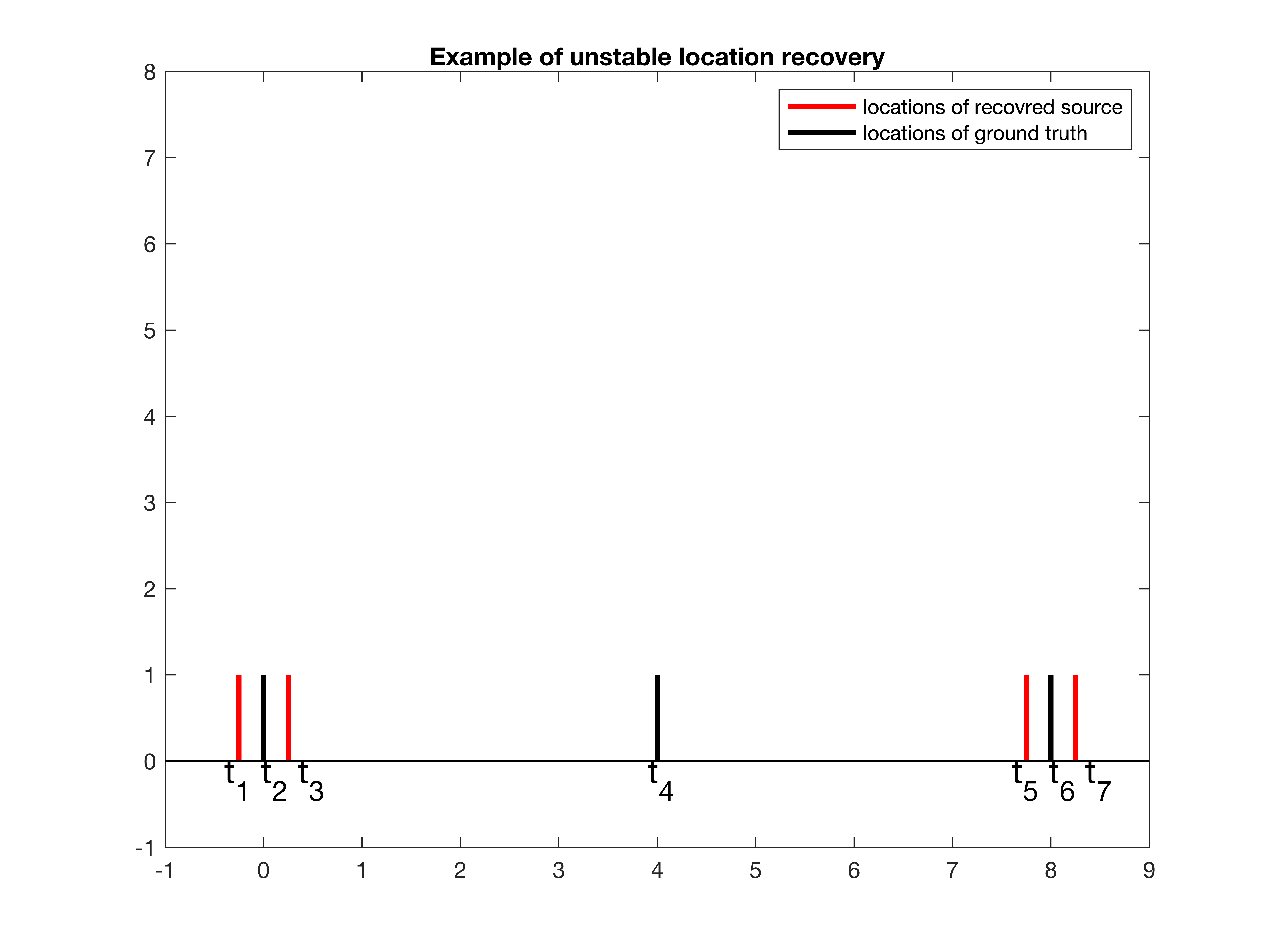
Refer to caption
Figure 2.1: An example of unstable location recovery.
Remark 2.1.

Note that all of our results hold for the case when the sources are supported on a grid. Specifically, we consider the grid points tj=jΔ,j=1,⋯,N,t_{j}=j\Delta,j=1,\cdots,N, where NN and Δ\Delta are the number and spacing of grid points, respectively, and assume the sources are supported on the grid. Assume also that the grid spacing Δ≤e−1Ω​(σmmin)12​n−1\Delta\leq\frac{e^{-1}}{\Omega}\left(\frac{\sigma}{m_{\min}}\right)^{\frac{1}{2n-1}} for fixed nn and mminm_{\min}. By Theorem 2.4, we can construct two positive measures μ=∑q=1naq​δtjq\mu=\sum_{q=1}^{n}a_{q}\delta_{t_{j_{q}}} and μ^=∑q=1na^q​δt^jq\hat{\mu}=\sum_{q=1}^{n}\hat{a}_{q}\delta_{\hat{t}_{j_{q}}} supported on the grid with completely different supports such that the difference of their Fourier data is less than the noise level and the minimum separation of sources is equal or less than 2​e−1Ω​(σmmin)12​n−1\frac{2e^{-1}}{\Omega}\left(\frac{\sigma}{m_{\min}}\right)^{\frac{1}{2n-1}} with minq=1,⋯,n⁡aq=mmin\min_{q=1,\cdots,n}a_{q}=m_{\min}.

Remark 2.2.

Note that our estimates for both the resolution limits in the number detection and support recovery already improve the estimates in [31] for the case of general sources.

2.1 Stability analysis of sparsity-promoting algorithms

Nowadays, sparsity-promoting algorithms are popular methods in image processing, signal processing and many other fields. By our results for the resolution limits, we can derive a sharp stability result for the l0l_{0} minimization in the super-resolution of positive sources. We consider the following l0l_{0}-minimization problem:

minρ supported on 𝒪, ρ is a positive discrete measure⁡||ρ||0subject to|ℱ​ρ​(ω)−𝐘⁡(ω)|<σ,ω∈[−Ω,Ω],\min_{\text{$\rho$ supported on $\mathcal{O}$, $\rho$ is a positive discrete measure}}\left|\left|{\rho}\right|\right|_{0}\quad\text{subject to}\quad|\mathcal{F}\rho(\omega)-\boldsymbol{\mathbf{Y}}(\omega)|<\sigma,\quad\omega\in[-\Omega,\Omega], (2.6)

where ‖ρ‖0||\rho||_{0} is the number of Dirac masses representing the discrete measure ρ\rho. As a corollary of Theorems 2.1 and 2.3, we have the following theorem for its stability.

Theorem 2.5.

Let n≥2n\geq 2 and σ≤mmin\sigma\leq m_{\min}. Let the measurement 𝐘\boldsymbol{\mathbf{Y}} in (1.1) be generated by a positive nn-sparse measure μ=∑j=1naj​δyj,yj∈I⁡(n,Ω)\mu=\sum_{j=1}^{n}a_{j}\delta_{y_{j}},y_{j}\in I(n,\Omega). Assume that

dmin:=minp≠j⁡|yp−yj|≥2.36​e​πΩ​(σmmin)12​n−1.d_{\min}:=\min_{p\neq j}\left|y_{p}-y_{j}\right|\geq\frac{2.36e\pi}{\Omega}\Big(\frac{\sigma}{m_{\min}}\Big)^{\frac{1}{2n-1}}. (2.7)

Let 𝒪\mathcal{O} in the minimization problem (2.6) be (or be included in) I⁡(n,Ω)I(n,\Omega) , then the solution to (2.6) contains exactly nn point sources. For any solution μ^=∑j=1na^j​δy^j\hat{\mu}=\sum_{j=1}^{n}\hat{a}_{j}\delta_{\hat{y}_{j}}, it is in a dmin2\frac{d_{\min}}{2}-neighborhood of μ\mu. Moreover, after reordering the y^j{\hat{y}}_{j}’s, we have

|y^j−yj|≤C⁡(n)Ω​S​R​F2​n−2​σmmin,1≤j≤n,\left|\hat{y}_{j}-y_{j}\right|\leq\frac{C(n)}{\Omega}SRF^{2n-2}\frac{\sigma}{m_{\min}},\quad 1\leq j\leq n, (2.8)

where C⁡(n)=C⁡(n)=22​n−32​e2​n−1​(max⁡(n−2,1)​π)−12C(n)=C(n)=2^{2n-\frac{3}{2}}e^{2n-1}(\max(\sqrt{n-2},1)\pi)^{-\frac{1}{2}}.

Theorem 2.5 reveals that sparsity promoting over admissible solutions can resolve the source locations to the resolution limit level. It provides an insight that theoretically sparsity-promoting algorithms would have excellent performance on the super-resolution of positive sources, which already have been corroborated by [35, 34, 13]. Especially, under the separation condition (2.7), any tractable sparsity-promoting algorithms (such as total variation minimization algorithms [7]) rendering the sparsest solution could stably reconstruct all the source locations.

3 Resolution limits for super-resolution in multi-dimensional spaces

In this section, combining the estimates in Section 2 and [30, 29], we present our main results on the resolution limits to the super-resolution of positive sources in multi-dimensional spaces. Let us first introduce the model setting. We consider the source as the nn-sparse positive measure

μ=∑j=1naj​δ𝐲j,\mu=\sum_{j=1}^{n}a_{j}\delta_{\boldsymbol{\mathbf{y}}_{j}},

where δ\delta denotes Dirac’s δ\delta-distribution in ℝk\mathbb{R}^{k}, 𝐲j∈ℝk,1≤j≤n\boldsymbol{\mathbf{y}}_{j}\in\mathbb{R}^{k},1\leq j\leq n, represent the locations of the point sources and aj>0,1≤j≤na_{j}>0,1\leq j\leq n are their amplitudes. Denote by

mmin=minj=1,⋯,n⁡|aj|,dmin=minp≠j⁡‖𝐲p−𝐲j‖2.m_{\min}=\min_{j=1,\cdots,n}|a_{j}|,\quad d_{\min}=\min_{p\neq j}||\boldsymbol{\mathbf{y}}_{p}-\boldsymbol{\mathbf{y}}_{j}||_{2}. (3.1)

The available measurement is the noisy Fourier data of μ\mu in a bounded region, that is,

𝐘⁡(𝝎)=ℱ⁡[μ]​(𝝎)+𝐖⁡(𝝎)=∑j=1naj​ei​𝐲j⋅𝝎+𝐖⁡(𝝎),𝝎∈ℝk,\mathbf{Y}(\boldsymbol{\mathbf{\omega}})=\mathcal{F}[\mu](\boldsymbol{\mathbf{\omega}})+\mathbf{W}(\boldsymbol{\mathbf{\omega}})=\sum_{j=1}^{n}a_{j}e^{i\boldsymbol{\mathbf{y}}_{j}\cdot\boldsymbol{\mathbf{\omega}}}+\mathbf{W}(\boldsymbol{\mathbf{\omega}}),\ \boldsymbol{\mathbf{\omega}}\in\mathbb{R}^{k}, (3.2)

where with slight abuse of notation ℱ​μ\mathcal{F}\mu denotes the Fourier transform of μ\mu in the kk-dimensional space, Ω\Omega is the cut-off frequency, and 𝐖\mathbf{W} is the noise. We assume that

‖𝐖⁡(𝝎)‖∞<σ,‖𝝎‖2≤Ω,||\mathbf{W}(\boldsymbol{\mathbf{\omega}})||_{\infty}<\sigma,\ ||\boldsymbol{\mathbf{\omega}}||_{2}\leq\Omega,

where σ\sigma is the noise level and ||f⁡(𝝎)||∞:=max𝝎∈ℝk,‖𝝎‖2≤Ω⁡|f⁡(𝝎)|\left|\left|{f(\boldsymbol{\mathbf{\omega}})}\right|\right|_{\infty}:=\max_{\boldsymbol{\mathbf{\omega}}\in\mathbb{R}^{k},||\boldsymbol{\mathbf{\omega}}||_{2}\leq\Omega}|f(\boldsymbol{\mathbf{\omega}})| in this section. We are interested in the resolution limit for resolving a cluster of tightly-spaced point sources. Thus, we denote by

Bδk(𝐱):={𝐲|𝐲∈ℝk,||𝐲−𝐱||2<δ},B_{\delta}^{k}(\boldsymbol{\mathbf{x}}):=\Big\{\mathbf{y}\ \Big|\ \mathbf{y}\in\mathbb{R}^{k},\ ||\boldsymbol{\mathbf{y}}-\boldsymbol{\mathbf{x}}||_{2}<\delta\Big\},

and assume that 𝐲j∈B(n−1)​π2​Ωk(𝟎),j=1,⋯,n\boldsymbol{\mathbf{y}}_{j}\in B_{\frac{(n-1)\pi}{2\Omega}}^{k}(\boldsymbol{\mathbf{0}}),j=1,\cdots,n, or equivalently ‖𝐲j‖2<(n−1)​π2​Ω||\boldsymbol{\mathbf{y}}_{j}||_{2}<\frac{(n-1)\pi}{2\Omega}.

We then define positive σ\sigma-admissible measures and computational resolution limits in the kk-dimensional space analogously to those in the one-dimensional case.

Definition 3.1.

Given measurement 𝐘\mathbf{Y}, we say that the positive measure μ^=∑j=1ma^j​δ𝐲^j,𝐲^j∈ℝk\hat{\mu}=\sum_{j=1}^{m}\hat{a}_{j}\delta_{\mathbf{\hat{y}}_{j}},\ \mathbf{\hat{y}}_{j}\in\mathbb{R}^{k}, is a positive σ\sigma-admissible discrete measure of 𝐘\ \mathbf{Y} if

||ℱ⁡[μ^]​(𝝎)−𝐘⁡(𝝎)||∞<σ,for all​‖𝝎‖2≤Ω,𝝎∈ℝk.\left|\left|{\mathcal{F}[\hat{\mu}](\boldsymbol{\mathbf{\omega}})-\boldsymbol{\mathbf{Y}}(\boldsymbol{\mathbf{\omega}})}\right|\right|_{\infty}<\sigma,\ \text{for all}\ ||\boldsymbol{\mathbf{\omega}}||_{2}\leq\Omega,\ \boldsymbol{\mathbf{\omega}}\in\mathbb{R}^{k}.

In particular, without the constraint on the positivity of the amplitudes, μ^\hat{\mu} is called a σ\sigma-admissible discrete measure of 𝐘\ \mathbf{Y}.

Definition 3.2.

The computational resolution limit to the number detection problem in kk-dimensional space is defined as the smallest nonnegative number 𝒟k,n​u​m+\mathcal{D}_{k,num}^{+} such that for all positive nn-sparse measures ∑j=1naj​δ𝐲j,𝐲j∈B(n−1)​π2​Ωk​(𝟎)\sum_{j=1}^{n}a_{j}\delta_{\mathbf{y}_{j}},\boldsymbol{\mathbf{y}}_{j}\in B_{\frac{(n-1)\pi}{2\Omega}}^{k}(\boldsymbol{\mathbf{0}}) and the associated measurement 𝐘\boldsymbol{\mathbf{Y}} in (3.2), if

minp≠j⁡‖𝐲j−𝐲p‖2≥𝒟k,n​u​m+,\min_{p\neq j}||\mathbf{y}_{j}-\mathbf{y}_{p}||_{2}\geq\mathcal{D}_{k,num}^{+},

then there does not exist any positive σ\sigma-admissible measure with less than nn supports for 𝐘\mathbf{Y}. Note that if we remove the constraint of positivity on the source and the σ\sigma-admissible measure, the computational resolution limit is denoted by 𝒟k,n​u​m\mathcal{D}_{k,num}.

As a consequence of [30, Theorem 2.3], we have the following result for the upper bound of the 𝒟k,n​u​m+\mathcal{D}_{k,num}^{+}.

Theorem 3.1.

Let n≥2n\geq 2 and the measurement 𝐘\mathbf{Y} in (3.2) be generated by a positive nn-sparse measure μ=∑j=1naj​δ𝐲j,𝐲j∈B(n−1)​π2​Ωk​(𝟎)\mu=\sum_{j=1}^{n}a_{j}\delta_{\mathbf{y}_{j}},\boldsymbol{\mathbf{y}}_{j}\in B_{\frac{(n-1)\pi}{2\Omega}}^{k}(\boldsymbol{\mathbf{0}}). There is a constant Cn​u​m​(k,n)C_{num}(k,n) which has an explicit form such that if

minp≠j,1≤p,j≤n⁡||𝐲p−𝐲j||2≥Cn​u​m​(k,n)Ω​(σmmin)12​n−2\min_{p\neq j,1\leq p,j\leq n}\left|\left|{\mathbf{y}_{p}-\mathbf{y}_{j}}\right|\right|_{2}\geq\frac{C_{num}(k,n)}{\Omega}\Big(\frac{\sigma}{m_{\min}}\Big)^{\frac{1}{2n-2}} (3.3)

holds, then there do not exist any positive σ\sigma-admissible measures of  𝐘\mathbf{Y} with less than nn supports.

We next show that the above upper bound is optimal in terms of the signal-to-noise ratio.

Theorem 3.2.

For given 0<σ≤mmin0<\sigma\leq m_{\min} and integer n≥2n\geq 2, there exist positive measures μ=∑j=1naj​δ𝐲j\mu=\sum_{j=1}^{n}a_{j}\delta_{\boldsymbol{\mathbf{y}}_{j}} with nn supports, and μ^=∑j=1n−1a^j​δ𝐲^j\hat{\mu}=\sum_{j=1}^{n-1}\hat{a}_{j}\delta_{\mathbf{\hat{y}}_{j}} with (n−1)(n-1) supports such that ‖ℱ⁡[μ^]−ℱ⁡[μ]‖∞<σ||\mathcal{F}[\hat{\mu}]-\mathcal{F}[\mu]||_{\infty}<\sigma. Moreover,

min1≤j≤n⁡|aj|=mmin,minp≠j⁡||𝐲p−𝐲j||2=2​e−1Ω​(σmmin)12​n−2.\min_{1\leq j\leq n}|a_{j}|=m_{\min},\quad\min_{p\neq j}\left|\left|{\boldsymbol{\mathbf{y}}_{p}-\boldsymbol{\mathbf{y}}_{j}}\right|\right|_{2}=\frac{2e^{-1}}{\Omega}\Big(\frac{\sigma}{m_{\min}}\Big)^{\frac{1}{2n-2}}.
Proof.

Consider γ=∑j=12​n−1aj​δ𝐭j\gamma=\sum_{j=1}^{2n-1}a_{j}\delta_{\boldsymbol{\mathbf{t}}_{j}} with 𝐭1=(−(n−1)τ,0,⋯,0),𝐭2=(−(n−2)τ,0,⋯,0),⋯,𝐭2​n−1=((n−1)τ,0,⋯,0)\boldsymbol{\mathbf{t}}_{1}=(-(n-1)\tau,0,\cdots,0),\boldsymbol{\mathbf{t}}_{2}=(-(n-2)\tau,0,\cdots,0),\cdots,\boldsymbol{\mathbf{t}}_{2n-1}=((n-1)\tau,0,\cdots,0) and τ=e−1Ω​(σmmin)12​n−2\tau=\frac{e^{-1}}{\Omega}\Big(\frac{\sigma}{m_{\min}}\Big)^{\frac{1}{2n-2}}. For every 𝝎=(ω1,ω2,⋯,ωk)⊤\boldsymbol{\mathbf{\omega}}=(\omega_{1},\omega_{2},\cdots,\omega_{k})^{\top},

ℱ​γ​(𝝎)=∑j=12​n−1aj​ei​𝐭j⋅𝝎=∑j=12​n−1aj​ei⁡(−n+j)​τ​ω1,|ω1|≤Ω.\mathcal{F}\gamma(\boldsymbol{\mathbf{\omega}})=\sum_{j=1}^{2n-1}a_{j}e^{i\boldsymbol{\mathbf{t}}_{j}\cdot\boldsymbol{\mathbf{\omega}}}=\sum_{j=1}^{2n-1}a_{j}e^{i(-n+j)\tau\omega_{1}},|\omega_{1}|\leq\Omega.

This reduces the estimation of ℱ​γ​(𝝎)\mathcal{F}\gamma(\boldsymbol{\mathbf{\omega}}) to the one-dimensional case. Combined with Theorem 2.2, there exist a2​j−1>0,a2​j<0,1≤j≤n,minj=1,⋯,n⁡|a2​j−1|=mmina_{2j-1}>0,a_{2j}<0,1\leq j\leq n,\min_{j=1,\cdots,n}|a_{2j-1}|=m_{\min}, so that ||ℱ​γ​(𝝎)||∞<σ\left|\left|{\mathcal{F}\gamma(\boldsymbol{\mathbf{\omega}})}\right|\right|_{\infty}<\sigma. As a consequence,

μ=∑j=1na2​j−1δ𝐭2​j−1,μ^=∑j=1n−1−a2​jδ𝐭2​j\mu=\sum_{j=1}^{n}a_{2j-1}\delta_{\boldsymbol{\mathbf{t}}_{2j-1}},\quad\hat{\mu}=\sum_{j=1}^{n-1}-a_{2j}\delta_{\boldsymbol{\mathbf{t}}_{2j}}

satisfy all the conditions of the theorem. ∎

The above results indicate that

C1,k​(n)Ω​(σmmin)12​n−2<𝒟k,n​u​m+≤C2,k​(n)Ω​(σmmin)12​n−2,\frac{C_{1,k}(n)}{\Omega}\Big(\frac{\sigma}{m_{\min}}\Big)^{\frac{1}{2n-2}}<\mathcal{D}_{k,num}^{+}\leq\frac{C_{2,k}(n)}{\Omega}\Big(\frac{\sigma}{m_{\min}}\Big)^{\frac{1}{2n-2}},

with C1,k​(n),C2,k​(n)C_{1,k}(n),C_{2,k}(n) being certain constants. An interesting open problem is to improve these constants. Two of the authors of this paper have made a progress in this direction [29].

To state the estimates for the resolution limits to the location recovery, we introduce the following concepts which are analogue to those in the one-dimensional case.

Definition 3.3.

Let μ=∑j=1naj​δ𝐲j\mu=\sum_{j=1}^{n}a_{j}\delta_{\boldsymbol{\mathbf{y}}_{j}} be a positive nn-sparse discrete measure in ℝk\mathbb{R}^{k} and let δ>0\delta>0 be such that the nn balls Bδk​(𝐲j),1≤j≤n,B_{\delta}^{k}(\boldsymbol{\mathbf{y}}_{j}),1\leq j\leq n, are pairwise disjoint. We say that μ^=∑j=1na^j​δ𝐲^j\hat{\mu}=\sum_{j=1}^{n}\hat{a}_{j}\delta_{\mathbf{\hat{y}}_{j}} is within δ\delta-neighborhood of μ\mu if each 𝐲^j\mathbf{\hat{y}}_{j} is contained in one and only one of the nn balls Bδk​(𝐲j),1≤j≤nB_{\delta}^{k}(\boldsymbol{\mathbf{y}}_{j}),1\leq j\leq n.

Definition 3.4.

The computational resolution limit to the stable support recovery problem in kk-dimensional space is defined as the smallest non-negative number 𝒟k,s​u​p​p+\mathcal{D}_{k,supp}^{+} such that for any positive nn-sparse measure μ=∑j=1naj​δ𝐲j,𝐲j∈B(n−1)​π2​Ωk​(𝟎)\mu=\sum_{j=1}^{n}a_{j}\delta_{\mathbf{y}_{j}},\boldsymbol{\mathbf{y}}_{j}\in B_{\frac{(n-1)\pi}{2\Omega}}^{k}(\boldsymbol{\mathbf{0}}) and the associated measurement 𝐘\boldsymbol{\mathbf{Y}} in (3.2), if

minp≠j,1≤p,j≤n⁡||𝐲p−𝐲j||2≥𝒟k,s​u​p​p+,\min_{p\neq j,1\leq p,j\leq n}\left|\left|{\mathbf{y}_{p}-\mathbf{y}_{j}}\right|\right|_{2}\geq\mathcal{D}_{k,supp}^{+},

then there exists δ>0\delta>0 such that any σ\sigma-admissible measure of 𝐘\mathbf{Y} with nn supports in B(n−1)​π2​Ωk​(𝟎)B_{\frac{(n-1)\pi}{2\Omega}}^{k}(\mathbf{0}) is within a δ\delta-neighbourhood of μ\mu.

As a consequence of [30, Theorem 2.7], we have the following result on the characterization of 𝒟k,s​u​p​p+\mathcal{D}_{k,supp}^{+}.

Theorem 3.3.

Let n≥2n\geq 2. Let the measurement 𝐘\boldsymbol{\mathbf{Y}} in (3.2) be generated by a positive nn-sparse measure μ=∑j=1naj​δ𝐲j,𝐲j∈B(n−1)​π2​Ωk​(𝟎)\mu=\sum_{j=1}^{n}a_{j}\delta_{\boldsymbol{\mathbf{y}}_{j}},\boldsymbol{\mathbf{y}}_{j}\in B_{\frac{(n-1)\pi}{2\Omega}}^{k}(\boldsymbol{\mathbf{0}}) in the kk-dimensional space. There is a constant Cs​u​p​p​(k,n)C_{supp}(k,n) which has an explicit form such that if

dmin:=minp≠j⁡‖𝐲p−𝐲j‖2≥Cs​u​p​p​(k,n)Ω​(σmmin)12​n−1d_{\min}:=\min_{p\neq j}\Big|\Big|\mathbf{y}_{p}-\mathbf{y}_{j}\Big|\Big|_{2}\geq\frac{C_{supp}(k,n)}{\Omega}\Big(\frac{\sigma}{m_{\min}}\Big)^{\frac{1}{2n-1}} (3.4)

holds, then for any μ^=∑j=1na^j​δ𝐲^j,𝐲^j∈B(n−1)​π2​Ωk​(𝟎)\hat{\mu}=\sum_{j=1}^{n}\hat{a}_{j}\delta_{\mathbf{\hat{y}}_{j}},\mathbf{\hat{y}}_{j}\in B_{\frac{(n-1)\pi}{2\Omega}}^{k}(\boldsymbol{\mathbf{0}}) being a positive σ\sigma-admissible measure of 𝐘\boldsymbol{\mathbf{Y}}, μ^\hat{\mu} is within the dmin2\frac{d_{\min}}{2}-neighborhood of μ\mu. Moreover, after reordering the 𝐲^j\mathbf{\hat{y}}_{j}’s, we have

‖𝐲^j−𝐲j‖2≤C⁡(k,n)Ω​S​R​F2​n−2​σmmin,1≤j≤n,\Big|\Big|\mathbf{\hat{y}}_{j}-\mathbf{y}_{j}\Big|\Big|_{2}\leq\frac{C(k,n)}{\Omega}SRF^{2n-2}\frac{\sigma}{m_{\min}},\quad 1\leq j\leq n, (3.5)

where S​R​F:=πΩSRF:=\frac{\pi}{\Omega} is the super-resolution factor and C⁡(k,n)C(k,n) has an explicit form.

Theorem 3.3 gives an upper bound for the computational resolution limit for the stable support recovery in the kk-dimensional space. This bound is optimal in terms of the order of the signal-to-noise ratio, as is shown by the theorem below.

Theorem 3.4.

For given 0<σ≤mmin0<\sigma\leq m_{\min} and integer n≥2n\geq 2, let

τ=e−1Ω​(σmmin)12​n−1.\tau=\frac{e^{-1}}{\Omega}\ \Big(\frac{\sigma}{m_{\min}}\Big)^{\frac{1}{2n-1}}. (3.6)

Then there exist a positive measure μ=∑j=1naj​δ𝐲j,𝐲j∈ℝk,\mu=\sum_{j=1}^{n}a_{j}\delta_{\boldsymbol{\mathbf{y}}_{j}},\boldsymbol{\mathbf{y}}_{j}\in\mathbb{R}^{k}, with nn supports at {(−(n−12)​τ,0,⋯,0),(−(n−52)​τ,0,⋯,0),⋯,((n−32)​τ,0,⋯,0)}\{(-(n-\frac{1}{2})\tau,0,\cdots,0),(-(n-\frac{5}{2})\tau,0,\cdots,0),\cdots,((n-\frac{3}{2})\tau,0,\cdots,0)\} and a positive measure μ^=∑j=1na^j​δ𝐲^j,𝐲^j∈ℝk,\hat{\mu}=\sum_{j=1}^{n}\hat{a}_{j}\delta_{\mathbf{\hat{y}}_{j}},\mathbf{\hat{y}}_{j}\in\mathbb{R}^{k}, with nn supports at {(−(n−32)​τ,0,⋯,0),(−(n−72)​τ,0,⋯,0),⋯,((n−12)​τ,0,⋯,0)}\{(-(n-\frac{3}{2})\tau,0,\cdots,0),(-(n-\frac{7}{2})\tau,0,\cdots,0),\cdots,((n-\frac{1}{2})\tau,0,\cdots,0)\} such that

||ℱ⁡[μ^]−ℱ⁡[μ]||∞<σ,min1≤j≤n⁡|aj|=mmin.\left|\left|{\mathcal{F}[\hat{\mu}]-\mathcal{F}[\mu]}\right|\right|_{\infty}<\sigma,\quad\min_{1\leq j\leq n}|a_{j}|=m_{\min}.
Proof.

Similar to the discussions in the proof of Theorem 3.2, the problem can be reduced to the one-dimensional case. Then leveraging Theorem 2.4 proves the result. ∎

Theorem 3.4 provides a lower bound to the computational resolution limit 𝒟k,s​u​p​p+\mathcal{D}_{k,supp}^{+}. Combined with Theorem 3.3, it reveals that

C3,k​(n)Ω​(σmmin)12​n−1<𝒟k,s​u​p​p+≤C4,k​(n)Ω​(σmmin)12​n−1\frac{C_{3,k}(n)}{\Omega}\ \Big(\frac{\sigma}{m_{\min}}\Big)^{\frac{1}{2n-1}}<\mathcal{D}_{k,supp}^{+}\leq\frac{C_{4,k}(n)}{\Omega}\Big(\frac{\sigma}{m_{\min}}\Big)^{\frac{1}{2n-1}}

for certain constants C3,k​(n),C4,k​(n)C_{3,k}(n),C_{4,k}(n).

Remark 3.1.

Compared to the one-dimensional case in Section 2, the upper bounds of multi-dimensional computational resolution limits for the number detection and location recovery in the super-resolution of positive sources has the same dependence on the signal-to-noise ratio and cutoff frequency. Moreover, their dependence on the dimensionality are indicated by the constant factors in the upper bound. We conjecture that the optimal constants may be independent of the source number nn. Note that the constant factors in the bounds have been improved in [29] to nearly optimal for the two-dimensional case.

4 Does the positivity enhace the resolution limit?

It is indicated in previous theorems that the a priori information of positivity cannot further improve the resolution order as compared to the case of complex sources [31, 28]. A further question is whether the positivity can indeed improve the resolution limit or not. To answer the question, in this section we demonstrate that, in certain scenarios, positivity actually deteriorates the resolution limit. Specifically, we show that two point sources with different phases can have a better resolution limit than those with the same phase.

We first consider a generalized diffraction limit problem. Note that the classic diffraction limit problem considers distinguishing two positive sources with identical intensities [1, 38, 41, 44]. However, in order to highlight the effect of the phase difference between two sources, we introduce a generalized diffraction limit that examines the ability to resolve two sources with equal magnitudes but varying phases.

Definition 4.1.

The generalized two-point diffraction limit is defined as the largest nonnegative number ℛ⁡(θ)\mathcal{R}(\theta) such that for all measures μ=∑j=12aj​δ𝐲j,𝐲j∈ℝk\mu=\sum_{j=1}^{2}a_{j}\delta_{\boldsymbol{\mathbf{y}}_{j}},\boldsymbol{\mathbf{y}}_{j}\in\mathbb{R}^{k} with |a1|=|a2|>0|a_{1}|=|a_{2}|>0 and the phase difference of a1,a2a_{1},a_{2} being θ\theta, if

||𝐲1−𝐲2||2<ℛ⁡(θ),\left|\left|{\boldsymbol{\mathbf{y}}_{1}-\boldsymbol{\mathbf{y}}_{2}}\right|\right|_{2}<\mathcal{R}(\theta),

then, for some image 𝐘\boldsymbol{\mathbf{Y}} in the model (3.2), it is impossible to determine whether the image 𝐘\boldsymbol{\mathbf{Y}} is generated from one or two sources from the σ\sigma-admissible measures defined in Definition 3.1. In other words, there exists a σ\sigma-admissible measure of some 𝐘\boldsymbol{\mathbf{Y}} with only one point source.

By the above definition, when ||𝐲1−𝐲2||2≥ℛ⁡(θ)\left|\left|{\boldsymbol{\mathbf{y}}_{1}-\boldsymbol{\mathbf{y}}_{2}}\right|\right|_{2}\geq\mathcal{R}(\theta), one can definitely distinguish two points with amplitudes of the same magnitude and a phase difference θ\theta from their image. Conversely, if the separation condition fails to hold, in some cases it is impossible to determine if the image is generated from one or two sources. We have the following theorem for the exact characterization of this generalized two-point diffraction.

Theorem 4.1.

Consider the collection of two sources μ=a1δ𝐲1+a2δ𝐲2,yj∈ℝk,j=1,2\mu=a_{1}\delta_{\boldsymbol{\mathbf{y}}_{1}}+a_{2}\delta_{\boldsymbol{\mathbf{y}}_{2}},y_{j}\in\mathbb{R}^{k},j=1,2 with a1=mmin​ei​θ1,a2=mmin​ei​θ2a_{1}=m_{\min}e^{i\theta_{1}},a_{2}=m_{\min}e^{i\theta_{2}}. Denote by θ=|θ1−θ2|\theta=\left|{\theta_{1}-\theta_{2}}\right| and assume that θ∈[0,π2]\theta\in\left[0,\frac{\pi}{2}\right]. When sin⁡(θ2)2≤σmmin≤12\sin\left(\frac{\theta}{2}\right)^{2}\leq\frac{\sigma}{m_{\min}}\leq\frac{1}{2}, the generalized two-point diffraction limit ℛ⁡(θ)\mathcal{R}(\theta) in a space of general dimensionality is given by

ℛ⁡(θ)=4​arcsin⁡((σmmin)12)−θΩ.\mathcal{R}(\theta)=\frac{4\arcsin\left(\left(\frac{\sigma}{m_{\min}}\right)^{\frac{1}{2}}\right)-\theta}{\Omega}. (4.1)

When σmmin>12\frac{\sigma}{m_{\min}}>\frac{1}{2}, no matter what the separation distance is, there are always some σ\sigma-admissible measures of some image 𝐘\boldsymbol{\mathbf{Y}} with only one point source.

Theorem 4.1 precisely characterizes the resolution of two points with the same magnitude but with a phase difference in [0,π2][0,\frac{\pi}{2}] under certain noise level. In particular, it reveals an interesting fact that sometimes two sources with identical amplitudes have the worst diffraction limit. Therefore, the phase difference actually improves the resolution limit.

However, Theorem 4.1 has a specific setting, and it is more crucial to determine the resolution limit for general scenarios. In the ensuing theorem, we investigate the computational resolution limit while considering phase differences between sources. It is worth noting that the original definition of the computational resolution limit does not include the phase difference. Still, we have utilized the same notion to avoid any confusion.

Theorem 4.2.

For θ∈[0,π2]\theta\in[0,\frac{\pi}{2}] and sin⁡(θ2)2≤σmmin≤12\sin\left(\frac{\theta}{2}\right)^{2}\leq\frac{\sigma}{m_{\min}}\leq\frac{1}{2}, the resolution limit 𝒟k,n​u​m\mathcal{D}_{k,num} for resolving two sources with phase difference θ\theta in ℝk\mathbb{R}^{k} is given by

𝒟k,n​u​m=4​arcsin⁡((σmmin)12)−θΩ.\mathcal{D}_{k,num}=\frac{4\arcsin\left(\left(\frac{\sigma}{m_{\min}}\right)^{\frac{1}{2}}\right)-\theta}{\Omega}. (4.2)

It can be attained if |a1|=|a2||a_{1}|=|a_{2}|. When σmmin>12\frac{\sigma}{m_{\min}}>\frac{1}{2}, no matter what the separation distance is, there are always some σ\sigma-admissible measures of some 𝐘\boldsymbol{\mathbf{Y}} with only one point source.

Theorem 4.2 establishes that, under certain noise levels, when there is a phase difference between two sources, their computational resolution limit is strictly better than that of two positive sources; this means that positivity actually impairs the resolution limit rather than improving it. It is also worth noting that, as per Theorem 4.2, super-resolution can already be achieved to some extent provided that σmmin<12\frac{\sigma}{m_{\min}}<\frac{1}{2}, especially when the source amplitudes differ in phase.

5 Phase transition in the number detection

In this section, employing the sweeping singular-value-thresholding number detection algorithm introduced in [31], we verify the phase transition phenomenon for the number detection in the super-resolution of positive sources.

5.1 Review of the sweeping singular-value-thresholding number detection algorithm

In [31], the authors proposed a number detection algorithm called sweeping single-value-thresholding number detection algorithm. It determines the number of sources by thresholding on the singular value of a Hankel matrix formulated from the measurement data.

To be more specific, suppose the measurement is taken at MM evenly-spaced points ω1=−Ω,ω2,⋯,ωM=Ω\omega_{1}=-\Omega,\omega_{2},\cdots,\omega_{M}=\Omega, that is,

𝐘(ωj)=ℱμ(ωj)+𝐖(ωj),j=1,⋯,M.\mathbf{Y}(\omega_{j})=\mathcal{F}\mu(\omega_{j})+\mathbf{W}(\omega_{j}),\quad j=1,\cdots,M.

We choose a partial measurement at the sample points zt=ω(t−1)​r+1z_{t}=\omega_{(t-1)r+1} for t=1,⋯,2​s+1t=1,\cdots,2s+1, where s≥ns\geq n and r=(M−1)mod2​sr=(M-1)\mod 2s. For ease of exposition, assume r=M−12​sr=\frac{M-1}{2s}. Then zt=ω(t−1)​M−12​s+1=−Ω+t−1s​Ωz_{t}=\omega_{(t-1)\frac{M-1}{2s}+1}=-\Omega+\frac{t-1}{s}\Omega (since ω1=−Ω\omega_{1}=-\Omega, ωM=Ω\omega_{M}=\Omega) and the partial measurement is

𝐘⁡(zt)=ℱ​μ​(zt)+𝐖⁡(zt),1≤t≤2​s+1.\mathbf{Y}(z_{t})=\mathcal{F}\mu(z_{t})+\mathbf{W}(z_{t}),\quad 1\leq t\leq 2s+1.

Assemble the following Hankel matrix by the measurements that

𝐇⁡(s)=(𝐘⁡(−Ω)𝐘⁡(−Ω+1s​Ω)⋯𝐘⁡(0)𝐘⁡(−Ω+1s​Ω)𝐘⁡(−Ω+2s​Ω)⋯𝐘⁡(1s​Ω)⋯⋯⋱⋯𝐘⁡(0)𝐘⁡(1s​Ω)⋯𝐘⁡(Ω)).\mathbf{H}(s)=\left(\begin{array}[]{cccc}\mathbf{Y}(-\Omega)&\mathbf{Y}(-\Omega+\frac{1}{s}\Omega)&\cdots&\mathbf{Y}(0)\\ \mathbf{Y}(-\Omega+\frac{1}{s}\Omega)&\mathbf{Y}(-\Omega+\frac{2}{s}\Omega)&\cdots&\mathbf{Y}(\frac{1}{s}\Omega)\\ \cdots&\cdots&\ddots&\cdots\\ \mathbf{Y}(0)&\mathbf{Y}(\frac{1}{s}\Omega)&\cdots&\mathbf{Y}(\Omega)\end{array}\right). (5.1)

We observe that 𝐇⁡(s)\mathbf{H}(s) has the decomposition

𝐇⁡(s)=D​A​D⊤+Δ,\mathbf{H}(s)=DAD^{\top}+\Delta,

where A=diag​(e−i​y1​Ω​a1,⋯,e−i​yn​Ω​an)A=\text{diag}(e^{-iy_{1}\Omega}a_{1},\cdots,e^{-iy_{n}\Omega}a_{n}) and D=(ϕs​(ei​y1​Ωs),⋯,ϕs​(ei​yn​Ωs))D=\big(\phi_{s}(e^{iy_{1}\frac{\Omega}{s}}),\cdots,\phi_{s}(e^{iy_{n}\frac{\Omega}{s}})\big) with ϕs​(ω)\phi_{s}(\omega) being defined as (1,ω,⋯,ωs)⊤(1,\omega,\cdots,\omega^{s})^{\top} and

Δ=(𝐖⁡(−Ω)𝐖⁡(−Ω+1s​Ω)⋯𝐖⁡(0)𝐖⁡(−Ω+1s​Ω)𝐖⁡(−Ω+2s​Ω)⋯𝐖⁡(1s​Ω)⋮⋮⋱⋮𝐖⁡(0)𝐖⁡(1s​Ω)⋯𝐖⁡(Ω)).\Delta=\left(\begin{array}[]{cccc}\mathbf{W}(-\Omega)&\mathbf{W}(-\Omega+\frac{1}{s}\Omega)&\cdots&\mathbf{W}(0)\\ \mathbf{W}(-\Omega+\frac{1}{s}\Omega)&\mathbf{W}(-\Omega+\frac{2}{s}\Omega)&\cdots&\mathbf{W}(\frac{1}{s}\Omega)\\ \vdots&\vdots&\ddots&\vdots\\ \mathbf{W}(0)&\mathbf{W}(\frac{1}{s}\Omega)&\cdots&\mathbf{W}(\Omega)\end{array}\right).

We denote the singular value decomposition of 𝐇⁡(s)\mathbf{H}(s) as

𝐇⁡(s)=U^​Σ^​U^∗,\mathbf{H}(s)=\hat{U}\hat{\Sigma}\hat{U}^{*},

where Σ^=diag​(σ^1,⋯,σ^n,σ^n+1,⋯,σ^s+1)\hat{\Sigma}=\text{diag}(\hat{\sigma}_{1},\cdots,\hat{\sigma}_{n},\hat{\sigma}_{n+1},\cdots,\hat{\sigma}_{s+1}) with the singular values σ^j\hat{\sigma}_{j}, 1≤j≤s+11\leq j\leq s+1, ordered in a decreasing manner. From [31], we have the following theorem for the threshold to determine the source number.

Theorem 5.1.

Let s≥ns\geq n and μ=∑j=1naj​δyj\mu=\sum_{j=1}^{n}a_{j}\delta_{y_{j}} with yj∈I⁡(n,Ω),1≤j≤ny_{j}\in I(n,\Omega),1\leq j\leq n. We have

σ^j≤(s+1)σ,j=n+1,⋯,s+1.\hat{\sigma}_{j}\leq(s+1)\sigma,\quad j=n+1,\cdots,s+1. (5.2)

Moreover, if the following separation condition is satisfied

minp≠j⁡|yp−yj|>π​sΩ​(2​n​(s+1)ζ​(n)2​σmmin)12​n−2,\min_{p\neq j}|y_{p}-y_{j}|>\frac{\pi s}{\Omega}\Big(\frac{2n(s+1)}{\zeta(n)^{2}}\frac{\sigma}{m_{\min}}\Big)^{\frac{1}{2n-2}}, (5.3)

where ζ⁡(n)={(n−12!)2,n is odd,(n2)!​(k−22)!,n is even,\zeta(n)=\left\{\begin{array}[]{cc}(\frac{n-1}{2}!)^{2},&\text{$n$ is odd,}\\ (\frac{n}{2})!(\frac{k-2}{2})!,&\text{$n$ is even,}\end{array}\right. then

σ^n>(s+1)​σ.\hat{\sigma}_{n}>(s+1)\sigma. (5.4)

Based on this theorem, the threshold should be (s+1)​σ(s+1)\sigma and the following Algorithm 1 was proposed to detect the source number for fixed ss.

Input: Number ss, Noise level σ\sigma;
Input: measurement: 𝐘=(𝐘⁡(ω1),⋯,𝐘⁡(ωM))⊤\mathbf{Y}=(\mathbf{Y}(\omega_{1}),\cdots,\mathbf{Y}(\omega_{M}))^{\top};
1: r=(M−1)mod2​sr=(M-1)\mod 2s, 𝐘n​e​w=(𝐘⁡(ω1),𝐘⁡(ωr+1),⋯,𝐘⁡(ω2​s​r+1))⊤\mathbf{Y}_{new}=(\mathbf{Y}(\omega_{1}),\mathbf{Y}(\omega_{r+1}),\cdots,\mathbf{Y}(\omega_{2sr+1}))^{\top};
2: Formulate the (s+1)×(s+1)(s+1)\times(s+1) Hankel matrix 𝐇⁡(s)\mathbf{H}(s) from 𝐘n​e​w\mathbf{Y}_{new}, and compute the singular value of 𝐇⁡(s)\mathbf{H}(s) as σ^1,⋯,σ^s+1\hat{\sigma}_{1},\cdots,\hat{\sigma}_{s+1} distributed in a decreasing manner;
4: Determine nn by σ^n>(s+1)​σ\hat{\sigma}_{n}>(s+1)\sigma and σ^j≤(s+1)σ,j=n+1,⋯,s+1\hat{\sigma}_{j}\leq(s+1)\sigma,j=n+1,\cdots,s+1;
Return: nn.
Algorithm 1 Singular-value-thresholding number detection algorithm

In Algorithm 1, the s≥ns\geq n should be properly chosen to have a good resolution. To address this issue, a sweeping strategy was utilized and the following Algorithm 2 was proposed. It was shown in [31] that the Algorithm 2 achieves the optimal resolution order.

Input: Noise level σ\sigma, measurement: 𝐘=(𝐘⁡(ω1),⋯,𝐘⁡(ωM))⊤\mathbf{Y}=(\mathbf{Y}(\omega_{1}),\cdots,\mathbf{Y}(\omega_{M}))^{\top};
Input: nm​a​x=0n_{max}=0
for s=1:⌊M−12⌋s=1:\lfloor\frac{M-1}{2}\rfloor do
Input s,σ,𝐘s,\sigma,\mathbf{Y} to Algorithm 1, save the output of Algorithm 1 as nr​e​c​o​v​e​rn_{recover};
    if nr​e​c​o​v​e​r>nm​a​xn_{recover}>n_{max} then
   nm​a​x=nr​e​c​o​v​e​rn_{max}=n_{recover} Return nm​a​xn_{max}.
Algorithm 2 Sweeping singular-value-thresholding number detection algorithm

5.2 Phase transition

We know from Section 2 that the resolution limit to the number detection problem in super-resolution of positive sources is bounded from below and above by C1Ω​(σmmin)12​n−2\frac{C_{1}}{\Omega}(\frac{\sigma}{m_{\min}})^{\frac{1}{2n-2}} and C2Ω​(σmmin)12​n−2\frac{C_{2}}{\Omega}(\frac{\sigma}{m_{\min}})^{\frac{1}{2n-2}}, respectively for some constants C1,C2C_{1},C_{2}. This indeed implies a phase transition phenomenon in the problem. Specifically, recall that the super-resolution factor is S​R​F=πdmin​ΩSRF=\frac{\pi}{d_{\min}\Omega} and the mminσ\frac{m_{\min}}{\sigma} can be viewed as the signal-to-noise ratio S​N​RSNR. Taking the logarithm of both sides of the two bounds, we can conclude that the exact number detection is guaranteed if

log⁡(S​N​R)>(2​n−2)​log⁡(S​R​F)+(2​n−2)​log⁡C1π,\log(SNR)>(2n-2)\log(SRF)+(2n-2)\log\frac{C_{1}}{\pi},

and may fail if

log⁡(S​N​R)<(2​n−2)​log⁡(S​R​F)+(2​n−2)​log⁡C2π.\log(SNR)<(2n-2)\log(SRF)+(2n-2)\log\frac{C_{2}}{\pi}.

As a consequence, we expect that in the parameter space of log⁡S​N​R−log⁡S​R​F\log SNR-\log SRF, there exist two lines both with slope 2​n−22n-2 such that the number detection is successful for cases above the first line and unsuccessful for cases below the second. In the intermediate region between the two lines, the number detection can be either successful or unsuccessful from case to case. This is clearly demonstrated in the numerical experiments below.

We fix Ω=1\Omega=1 and consider nn point sources randomly spaced in [−(n−1)​π2,(n−1)​π2]\left[-\frac{(n-1)\pi}{2},\frac{(n-1)\pi}{2}\right] with positive amplitudes aja_{j}’s. The noise level is σ\sigma and the minimum separation distance between sources is dmind_{\min}. We perform 10000 random experiments (the randomness is in the choice of (dmin,σ,yj,aj)(d_{\min},\sigma,y_{j},a_{j})) to detect the source number based on Algorithm 2. Figure 5.1 shows the results for n=2,4,n=2,4, respectively. In each case, two lines of slope 2​n−22n-2 strictly separate the blue points (successful detection) and red points (unsuccessful detection) and in-between is the phase transition region. It clearly elucidates the phase transition phenomenon of Algorithm 2 and is consistent with our theory.

Refer to caption
(a) detection success
Refer to caption
(b) detection fail
Refer to caption
(c) phase transition region
Refer to caption
(d) detection success
Refer to caption
(e) detection fail
Refer to caption
(f) phase transition region
Figure 5.1: Plots of the successful and the unsuccessful number detection by Algorithm 2 depending on the relation between log⁡(S​R​F)\log(SRF) and log⁡(mminσ)\log(\frac{m_{\min}}{\sigma}). (a) illustrates that two positive point source can be exactly detected if log⁡(mminσ)\log(\frac{m_{\min}}{\sigma}) is above a line of slope 22 in the parameter space. Conversely, for the same case, (b) shows that the number detection fails if log⁡(mminσ)\log(\frac{m_{\min}}{\sigma}) falls below another line of slope 22. (c) highlights the phase transition region which is bounded by the black slashes in (a) and (b). (d),(e) and (f) illustrate parallel results for four positive point sources.

6 Phase transition in the location recovery

In this section, by the MUSIC algorithm we verify the phase transition phenomenon for the location recovery in the super-resolution of positive sources.

6.1 Review of the MUSIC algorithm

In this section we review the MUSIC algorithm. From the measurement 𝐘=(𝐘⁡(ω1),𝐘⁡(ω2),⋯,𝐘⁡(ωM))⊤\mathbf{Y}=(\mathbf{Y}(\omega_{1}),\mathbf{Y}(\omega_{2}),\cdots,\mathbf{Y}(\omega_{M}))^{\top} and M^=⌊M−12⌋\hat{M}=\lfloor\frac{M-1}{2}\rfloor, we assemble the (M^+1)×(M^+1)(\hat{M}+1)\times(\hat{M}+1) Hankel matrix,

𝐇=(𝐘⁡(ω1)𝐘⁡(ω2)⋯𝐘⁡(ωM^)𝐘⁡(ω2)𝐘⁡(ω3)⋯𝐘⁡(ωM^+1)⋯⋯⋱⋯𝐘⁡(ωM^)𝐘⁡(ωM^+1)⋯𝐘⁡(ω2​M^+1)).\boldsymbol{\mathbf{H}}=\begin{pmatrix}\mathbf{Y}(\omega_{1})&\mathbf{Y}(\omega_{2})&\cdots&\mathbf{Y}(\omega_{\hat{M}})\\ \mathbf{Y}(\omega_{2})&\mathbf{Y}(\omega_{3})&\cdots&\mathbf{Y}(\omega_{\hat{M}+1})\\ \cdots&\cdots&\ddots&\cdots\\ \mathbf{Y}(\omega_{\hat{M}})&\mathbf{Y}(\omega_{\hat{M}+1})&\cdots&\mathbf{Y}(\omega_{2\hat{M}+1})\end{pmatrix}. (6.1)

We perform the following singular value decomposition for 𝐇\boldsymbol{\mathbf{H}},

𝐇=U^​Σ^​U^∗=[U^1U^2]​diag​(σ^1,σ^2,⋯,σ^n,σ^n+1,⋯,σ^M^+1)​[U^1U^2]∗,\boldsymbol{\mathbf{H}}=\hat{U}\hat{\Sigma}\hat{U}^{*}=[\hat{U}_{1}\quad\hat{U}_{2}]\text{diag}(\hat{\sigma}_{1},\hat{\sigma}_{2},\cdots,\hat{\sigma}_{n},\hat{\sigma}_{n+1},\cdots,\hat{\sigma}_{\hat{M}+1})[\hat{U}_{1}\quad\hat{U}_{2}]^{*},

where U^1=(U^​(1),⋯,U^​(n)),U^2=(U^​(n+1),⋯,U^​(M^+1))\hat{U}_{1}=(\hat{U}(1),\cdots,\hat{U}(n)),\hat{U}_{2}=(\hat{U}(n+1),\cdots,\hat{U}(\hat{M}+1)) with nn being the source number. Then we denote the orthogonal projection to the space U^2\hat{U}_{2} by P^2​x=U^2​(U^2∗​x)\hat{P}_{2}x=\hat{U}_{2}(\hat{U}_{2}^{*}x). For a test vector Φ⁡(x)=(1,ei​h​x,⋯,ei​M^​h​x)⊤\Phi(x)=(1,e^{ihx},\cdots,e^{i\hat{M}hx})^{\top} with hh being the spacing parameter, we define the MUSIC imaging functional

J^​(x)=‖Φ⁡(x)‖2‖P^2​Φ​(x)‖2=‖Φ⁡(x)‖2‖U^2∗​Φ​(x)‖2.\displaystyle\hat{J}(x)=\frac{||\Phi(x)||_{2}}{||\hat{P}_{2}\Phi(x)||_{2}}=\frac{||\Phi(x)||_{2}}{||\hat{U}_{2}^{*}\Phi(x)||_{2}}.

The local maximizers of J^​(x)\hat{J}(x) indicate the locations of the point sources. In practice, we test evenly spaced points in a specified interval and plot the discrete imaging functional and then determine the source locations by detecting the peaks. We present the peak selection algorithm as Algorithm 4 and summarize the MUSIC algorithm in Algorithm 3 below.

Input: Measurements: 𝐘=(𝐘⁡(ω1),⋯,𝐘⁡(ωM))⊤\mathbf{Y}=(\mathbf{Y}(\omega_{1}),\cdots,\mathbf{Y}(\omega_{M}))^{\top}, sampling distance hh, source number nn;
Input: Region of test points [T​S,T​E][TS,TE] and spacing of test points T​P​STPS;
1: Let M^=⌊M−12⌋\hat{M}=\lfloor\frac{M-1}{2}\rfloor, formulate the (M^+1)×(M^+1)(\hat{M}+1)\times(\hat{M}+1) Hankel matrix X^\hat{X} from 𝐘\mathbf{Y};
2: Compute the singular vector of X^\hat{X} as U^​(1),U^​(2),⋯,U^​(M^+1)\hat{U}(1),\hat{U}(2),\cdots,\hat{U}(\hat{M}+1) and formulate the noise space U^2=(U^​(n+1),⋯,U^​(M^+1))\hat{U}_{2}=(\hat{U}(n+1),\cdots,\hat{U}(\hat{M}+1));
3: For test points xx’s in [T​S,T​E][TS,TE] evenly spaced by T​P​STPS, construct the test vector Φ⁡(x)=(1,ei​h​x,⋯,ei​M^​h​x)⊤\Phi(x)=(1,e^{ihx},\cdots,e^{i\hat{M}hx})^{\top};
4: Plot the MUSIC imaging functional J^​(x)=‖Φ⁡(x)‖2‖U^2∗​Φ​(x)‖2\hat{J}(x)=\frac{||\Phi(x)||_{2}}{||\hat{U}_{2}^{*}\Phi(x)||_{2}};
5: Select the peak locations y^j\hat{y}_{j}’s in the J^​(x)\hat{J}(x) by Algorithm 4;
Return y^j\hat{y}_{j}’s.
Algorithm 3 MUSIC algorithm
Input: Image I​M​G=(f⁡(x1),⋯,f⁡(xN))IMG=(f(x_{1}),\cdots,f(x_{N}));
Input: Peak compare range P​C​RPCR, differential compare range D​C​RDCR, differential compare threshold D​C​TDCT;
1: Initialize the Local maximum points L​M​P=[]LMP=[\ ], peak points P​P=[]PP=[\ ];
2: Differentiate the image I​M​GIMG to get the D​I​M​G=(f′​(x1),⋯,f′​(xN))DIMG=(f^{\prime}(x_{1}),\cdots,f^{\prime}(x_{N}));
3: for j=1:Nj=1:N do
if f⁡(xj)=max⁡(f⁡(xj−P​C​R),f⁡(xj−P​C​R+1),⋯,f⁡(xj+P​C​R))f(x_{j})=\max(f(x_{j-PCR}),f(x_{j-PCR+1}),\cdots,f(x_{j+PCR})) then
    L​M​PLMP appends xjx_{j};
       4: for xjx_{j} in L​M​PLMP do
if max⁡(|f′​(xj−D​C​R)|,|f′​(xj−D​C​R+1)|,⋯,|f′​(xj+D​C​R)|)≥D​C​T\max(|f^{\prime}(x_{j-DCR})|,|f^{\prime}(x_{j-DCR+1})|,\cdots,|f^{\prime}(x_{j+DCR})|)\geq DCT then
   P​PPP appends xjx_{j};
      Return: P​PPP.
Algorithm 4 Peak selection algorithm

6.2 Phase transition

The derived bounds for the resolution limit 𝒟s​u​p​p+\mathcal{D}_{supp}^{+} of the location recovery in the super-resolution of positive sources implies a phase transition in the problem. Taking the logarithm of both sides of the two bounds, we can draw a conclusion that the location recovery is stable if

log⁡(S​N​R)>(2​n−1)​log⁡(S​R​F)+(2​n−1)​log⁡C3π,\log(SNR)>(2n-1)\log(SRF)+(2n-1)\log\frac{C_{3}}{\pi},

and may be unstable if

log⁡(S​N​R)<(2​n−1)​log⁡(S​R​F)+(2​n−1)​log⁡C4π,\log(SNR)<(2n-1)\log(SRF)+(2n-1)\log\frac{C_{4}}{\pi},

for certain constants C3,C4C_{3},C_{4}. Similar to the number detection, we expect that in the parameter space of log⁡S​N​R−log⁡S​R​F\log SNR-\log SRF, there exist two lines both with slope 2​n−12n-1 such that the location recovery is stable for cases above the first line and unstable for cases below the second. This phase transition phenomenon has been demonstrated numerically using the Matrix Pencil method, MUSIC and ESPRIT in [5, 26, 24, 25] for resolving general sparse sources.

In what follows, we shall conduct numerical experiments to demonstrate the phase transition phenomenon for the MUSIC algorithm in the super-resolution of positive sources. For simplicity, we fix Ω=1\Omega=1 and consider n=2n=2 or 44 positive point sources separated with minimum separation dmind_{\min}. We perform 1000010000 random experiments (the randomness is in the choice of (dmin,σ,yj,aj)(d_{\min},\sigma,y_{j},a_{j}) to recover the source locations using Algorithm 3. The recovery is deemed stable only if nn locations y^j\hat{y}_{j}’s are recovered and they are in a dmin2\frac{d_{\min}}{2}-neighborhood of the ground truth; see Algorithm 5 for details in a single experiment. As is shown in Figure 6.1, in each case, two lines with slope 2​n−12n-1 strictly separate the blue points (stable recoveries) and red points (unstable recoveries), and in-between is the phase transition region. This is exactly the predicted phase transition phenomenon by our theory. It also demonstrates that the MUSIC can resolve the location of positive point sources with optimal resolution order.

Input: Sources μ=∑j=1naj​δyj\mu=\sum_{j=1}^{n}a_{j}\delta_{y_{j}}, source number nn;
Input: Measurements: 𝐘\mathbf{Y}
Input source number nn and measurement 𝐘\boldsymbol{\mathbf{Y}} to Algorithm 3 and save the output as y^1,⋯,y^k\hat{y}_{1},\cdots,\hat{y}_{k}, which are ordered in an increasing manner;
if k==n then
Compute the reconstruction error for the source location yjy_{j} that ej:=|y^j−yj|e_{j}:=|\hat{y}_{j}-y_{j}|;
    if maxj=1,⋯,n⁡ej<minp≠j⁡|yp−yj|2\max_{j=1,\cdots,n}e_{j}<\frac{\min_{p\neq j}|y_{p}-y_{j}|}{2} then
   Return Stableelse
   Return Unstableelse
Return Unstable.
Algorithm 5 A single experiment
Refer to caption
(a) recovery success
Refer to caption
(b) recovery fail
Refer to caption
(c) phase transition region
Refer to caption
(d) recovery success
Refer to caption
(e) recovery fail
Refer to caption
(f) phase transition region
Figure 6.1: Plots of the stable and the unstable location recoveries by Algorithm 3 in view of the relation between log⁡(S​R​F)\log(SRF) and log⁡(mminσ)\log(\frac{m_{\min}}{\sigma}). (a) illustrates that the locations of two positive point sources can be stably recovered if log⁡(mminσ)\log(\frac{m_{\min}}{\sigma}) is above a line of slope 33 in the parameter space. Conversely, for the same case, (b) shows that the locations cannot be stably recovered by MUSIC if log⁡(mminσ)\log(\frac{m_{\min}}{\sigma}) falls below another line of slope 33. (c) highlights the phase transition region which is bounded by the black slashes in (a) and (b). (d),(e) and (f) illustrate parallel results for four positive point sources.

7 Conclusions and future works

In this paper, we have introduced the resolution limit for respectively the number detection and the location recovery in the super-resolution of positive sources. We have quantitatively characterized the two limits by establishing their sharp upper and lower bounds. We have also verified the phase transition phenomena that predicted by our theory in the number detection and support recovery problems.

Our new technique provides a way to analyze the resolving capability of the super-resolution of positive sources. The applications of the technique introduced here to other problems will be presented in a near future.

8 Proofs of results in Section 2

We first introduce some notation and lemmas that are used in the following proofs. Set

ϕs​(t)=(1,t,⋯,ts)⊤.\phi_{s}(t)=\left(1,t,\cdots,t^{s}\right)^{\top}. (8.1)

We recall the Stirling formula that

2​π​nn+12​e−n≤n!≤e​nn+12​e−n.\sqrt{2\pi}n^{n+\frac{1}{2}}e^{-n}\leq n!\leq en^{n+\frac{1}{2}}e^{-n}. (8.2)
Lemma 8.1.

Let t1,⋯,tkt_{1},\cdots,t_{k} be kk different real numbers and let tt be a real number. We have

(Dk​(k−1)−1​ϕk−1​(t))j=Π1≤q≤k,q≠j​t−tqtj−tq,\left(D_{k}(k-1)^{-1}\phi_{k-1}(t)\right)_{j}=\Pi_{1\leq q\leq k,q\neq j}\frac{t-t_{q}}{t_{j}-t_{q}},

where Dk​(k−1):=(ϕk−1​(t1),⋯,ϕk−1​(tk))D_{k}(k-1):=\big(\phi_{k-1}(t_{1}),\cdots,\phi_{k-1}(t_{k})\big) with ϕk−1​(⋅)\phi_{k-1}(\cdot) defined by (8.1).

Proof.

This is [31, Lemma 5]. For the reader’s convenience, we present a simple proof here. We denote (Dk​(k−1)−1)j​q=bj​q\left(D_{k}(k-1)^{-1}\right)_{jq}=b_{jq}. Observe that

(Dk​(k−1)−1​ϕk−1​(t))j=∑q=1kbj​q​tq−1.\left(D_{k}(k-1)^{-1}\phi_{k-1}(t)\right)_{j}=\sum_{q=1}^{k}b_{jq}t^{q-1}.

We have

∑q=1kbj​q​(tp)q−1=δj​p,∀j,p=1,⋯,k,\sum_{q=1}^{k}b_{jq}(t_{p})^{q-1}=\delta_{jp},\ \forall j,p=1,\cdots,k,

where δj​p\delta_{jp} is the Kronecker delta function. Then the polynomial Pj​(x)=∑q=1kbj​q​xq−1P_{j}(x)=\sum_{q=1}^{k}b_{jq}x^{q-1} satisfies Pj​(t1)=0,⋯,Pj​(tj−1)=0,Pj​(tj)=1,Pj​(tj+1)=0,⋯,Pj​(tk)=0P_{j}(t_{1})=0,\cdots,P_{j}(t_{j-1})=0,P_{j}(t_{j})=1,P_{j}(t_{j+1})=0,\cdots,P_{j}(t_{k})=0. Therefore, it must be the Lagrange polynomial

Pj​(x)=Π1≤q≤k,q≠j​x−tqtj−tq.P_{j}(x)=\Pi_{1\leq q\leq k,q\neq j}\frac{x-t_{q}}{t_{j}-t_{q}}.

It follows that

(Dk​(k−1)−1​ϕk−1​(t))j=Π1≤q≤k,q≠j​t−tqtj−tq.\displaystyle\left(D_{k}(k-1)^{-1}\phi_{k-1}(t)\right)_{j}=\Pi_{1\leq q\leq k,q\neq j}\frac{t-t_{q}}{t_{j}-t_{q}}.

∎

8.1 Proof of Theorem 2.2

Proof.

Step 1. Let

τ=e−1Ω​(σmmin)12​n−2\tau=\frac{e^{-1}}{\Omega}\Big(\frac{\sigma}{m_{\min}}\Big)^{\frac{1}{2n-2}} (8.3)

and t1=−(n−1)τ,t2=−(n−2)τ,⋯,tn=0,tn+1=τ,⋯,t2​n−1=(n−1)τt_{1}=-(n-1)\tau,t_{2}=-(n-2)\tau,\cdots,t_{n}=0,t_{n+1}=\tau,\cdots,t_{2n-1}=(n-1)\tau. Consider the following system of linear equations:

A​a=0,Aa=0, (8.4)

where A=(ϕ2​n−3​(t1),⋯,ϕ2​n−3​(t2​n−1))A=\big(\phi_{2n-3}(t_{1}),\cdots,\phi_{2n-3}(t_{2n-1})\big) with ϕ2​n−3​(⋅)\phi_{2n-3}(\cdot) being defined by (8.1). Since AA is underdetermined, there exists a nontrivial solution a=(a1,⋯,a2​n−1)⊤a=(a_{1},\cdots,a_{2n-1})^{\top} to (8.4). By the linear independence of the any (2​n−2)(2n-2) column vectors of AA, we can show that all aja_{j}’s are nonzero. By a scaling of aa, we can assume that a2​n−1>0a_{2n-1}>0 and

min1≤j≤n⁡|a2​j−1|=mmin.\min_{1\leq j\leq n}|a_{2j-1}|=m_{\min}. (8.5)

We define

μ=∑j=1na2​j−1δt2​j−1,μ^=∑j=1n−1−a2​jδt2​j.\mu=\sum_{j=1}^{n}a_{2j-1}\delta_{t_{2j-1}},\quad\hat{\mu}=\sum_{j=1}^{n-1}-a_{2j}\delta_{t_{2j}}.

We shall show that the intensities in μ^\hat{\mu} and μ\mu are all positive and ‖ℱ⁡[μ^]−ℱ⁡[μ]‖∞<σ||\mathcal{F}[\hat{\mu}]-\mathcal{F}[\mu]||_{\infty}<\sigma in the subsequent steps.

Step 2. We first analyze the sign of each aj,j=1,⋯,2​n−1,a_{j},j=1,\cdots,2n-1, based on a2​n−1>0a_{2n-1}>0. The equation (8.4) implies that

−a2​n−1​ϕ2​n−3​(t2​n−1)=(ϕ2​n−3​(t1),⋯,ϕ2​n−3​(t2​n−2))​(a1,⋯,a2​n−2)⊤,-a_{2n-1}\phi_{2n-3}(t_{2n-1})=\big(\phi_{2n-3}(t_{1}),\cdots,\phi_{2n-3}(t_{2n-2})\big)(a_{1},\cdots,a_{2n-2})^{\top},

and hence

−a2​n−1​(ϕ2​n−3​(t1),⋯,ϕ2​n−3​(t2​n−2))−1​ϕ2​n−3​(t2​n−1)=(a1,⋯,a2​n−2)⊤.-a_{2n-1}\left(\phi_{2n-3}(t_{1}),\cdots,\phi_{2n-3}(t_{2n-2})\right)^{-1}\phi_{2n-3}(t_{2n-1})=(a_{1},\cdots,a_{2n-2})^{\top}.

Together with Lemma 8.1, we have

−a2​n−1​Π1≤q≤2​n−2,q≠j​t2​n−1−tqtj−tq=aj,-a_{2n-1}\Pi_{1\leq q\leq 2n-2,q\neq j}\frac{t_{2n-1}-t_{q}}{t_{j}-t_{q}}=a_{j}, (8.6)

for j=1,⋯,2​n−2j=1,\cdots,2n-2. Observe first that Π1≤q≤2​n−2,q≠j​(t2​n−1−tq)\Pi_{1\leq q\leq 2n-2,q\neq j}(t_{2n-1}-t_{q}) is always positive for 1≤j≤2​n−21\leq j\leq 2n-2. For j=2​n−2j=2n-2, since a2​n−1>0a_{2n-1}>0, −a2​n−1​Π1≤q≤2​n−2,q≠2​n−2​(t2​n−2−tq)-a_{2n-1}\Pi_{1\leq q\leq 2n-2,q\neq 2n-2}(t_{2n-2}-t_{q}) is negative in (8.6). Thus we have a2​n−2<0a_{2n-2}<0. In the same fashion, we see that aj<0a_{j}<0 for even jj and aj>0a_{j}>0 for odd jj. Hence the intensities in μ^\hat{\mu} and μ\mu are all positive.

Step 3. We demonstrate that ‖ℱ⁡[μ^]−ℱ⁡[μ]‖∞<σ||\mathcal{F}[\hat{\mu}]-\mathcal{F}[\mu]||_{\infty}<\sigma. Observe that

‖ℱ⁡[μ^]−ℱ⁡[μ]‖∞=maxx∈[−Ω,Ω]⁡|ℱ⁡(γ)​(x)|,||\mathcal{F}[\hat{\mu}]-\mathcal{F}[\mu]||_{\infty}=\max_{x\in[-\Omega,\Omega]}|\mathcal{F}(\gamma)(x)|, (8.7)

where γ=∑j=12​n−1aj​δtj\gamma=\sum_{j=1}^{2n-1}a_{j}\delta_{t_{j}} and

ℱ⁡[γ]​(x)=∑j=12​n−1aj​ei​tj​x=∑j=12​n−1aj​∑k=0∞(i​tj​x)kk!=∑k=0∞Qk​(γ)​(i​x)kk!.\mathcal{F}[\gamma](x)=\sum_{j=1}^{2n-1}a_{j}e^{it_{j}x}=\sum_{j=1}^{2n-1}a_{j}\sum_{k=0}^{\infty}\frac{(it_{j}x)^{k}}{k!}=\sum_{k=0}^{\infty}Q_{k}(\gamma)\frac{(ix)^{k}}{k!}. (8.8)

Here, Qk​(γ)=∑j=12​n−1aj​tjkQ_{k}(\gamma)=\sum_{j=1}^{2n-1}a_{j}t_{j}^{k}. By (8.4), we have Qk(γ)=0,k=0,⋯,2n−3Q_{k}(\gamma)=0,k=0,\cdots,2n-3. We next estimate Qk​(γ)Q_{k}(\gamma) for k>2​n−3k>2n-3.

Step 4. We estimate ∑j=12​n−1|aj|\sum_{j=1}^{2n-1}|a_{j}| first. We begin by ordering aja_{j}’s such that

mmin=|aj1|≤|aj2|≤⋯≤|aj2​n−1|.m_{\min}=|a_{j_{1}}|\leq|a_{j_{2}}|\leq\cdots\leq|a_{j_{2n-1}}|.

Then (8.4) implies that

aj1​ϕ2​n−3​(tj1)=(ϕ2​n−3​(tj2),⋯,ϕ2​n−3​(tj2​n−1))​(−aj2,⋯,−aj2​n−1)⊤,a_{j_{1}}\phi_{2n-3}(t_{j_{1}})=\big(\phi_{2n-3}(t_{j_{2}}),\cdots,\phi_{2n-3}(t_{j_{2n-1}})\big)(-a_{j_{2}},\cdots,-a_{j_{2n-1}})^{\top},

and hence

aj1​(ϕ2​n−3​(tj2),⋯,ϕ2​n−3​(tj2​n−1))−1​ϕ2​n−3​(tj1)=(−aj2,⋯,−aj2​n−1)⊤.a_{j_{1}}\left(\phi_{2n-3}(t_{j_{2}}),\cdots,\phi_{2n-3}(t_{j_{2n-1}})\right)^{-1}\phi_{2n-3}(t_{j_{1}})=(-a_{j_{2}},\cdots,-a_{j_{2n-1}})^{\top}.

Together with Lemma 8.1, we have

aj1​Π2≤q≤2​n−2​tj1−tjqtj2​n−1−tjq=−aj2​n−1.a_{j_{1}}\Pi_{2\leq q\leq 2n-2}\frac{t_{j_{1}}-t_{j_{q}}}{t_{j_{2n-1}}-t_{j_{q}}}=-a_{j_{2n-1}}.

Further,

|aj2​n−1|=\displaystyle\left|{a_{j_{2n-1}}}\right|= |aj1|​Π2≤q≤2​n−2​|tj1−tjq||tj2​n−1−tjq|=|aj1|​Π2≤q≤2​n−2​|tj1−tjq||tj2​n−1−tjq|​|tj1−tj2​n−1||tj2​n−1−tj1|\displaystyle\left|{a_{j_{1}}}\right|\Pi_{2\leq q\leq 2n-2}\frac{\left|{t_{j_{1}}-t_{j_{q}}}\right|}{\left|{t_{j_{2n-1}}-t_{j_{q}}}\right|}=\left|{a_{j_{1}}}\right|\Pi_{2\leq q\leq 2n-2}\frac{\left|{t_{j_{1}}-t_{j_{q}}}\right|}{\left|{t_{j_{2n-1}}-t_{j_{q}}}\right|}\frac{\left|{t_{j_{1}}-t_{j_{2n-1}}}\right|}{\left|{t_{j_{2n-1}}-t_{j_{1}}}\right|} (8.9)
=\displaystyle= |aj1|​Π2≤q≤2​n−1​|tj1−tjq|Π1≤q≤2​n−2​|tj2​n−1−tjq|≤|aj1|​maxj1=1,⋯,2​n−1⁡Π2≤q≤2​n−1​|tj1−tjq|minj2​n−1=1,⋯,2​n−1⁡Π1≤q≤2​n−2​|tj2​n−1−tjq|.\displaystyle\left|{a_{j_{1}}}\right|\frac{\Pi_{2\leq q\leq 2n-1}\left|{t_{j_{1}}-t_{j_{q}}}\right|}{\Pi_{1\leq q\leq 2n-2}\left|{t_{j_{2n-1}}-t_{j_{q}}}\right|}\leq\left|{a_{j_{1}}}\right|\frac{\max_{j_{1}=1,\cdots,2n-1}\Pi_{2\leq q\leq 2n-1}\left|{t_{j_{1}}-t_{j_{q}}}\right|}{\min_{j_{2n-1}=1,\cdots,2n-1}\Pi_{1\leq q\leq 2n-2}\left|{t_{j_{2n-1}}-t_{j_{q}}}\right|}.

Thus, based on the distribution of tjt_{j}’s and (8.5), we have

|aj2​n−1|≤(2​n−2)!((n−1)!)2​|aj1|≤(2​n−2)!((n−1)!)2​mmin,|a_{j_{2n-1}}|\leq\frac{(2n-2)!}{\left((n-1)!\right)^{2}}|a_{j_{1}}|\leq\frac{(2n-2)!}{\left((n-1)!\right)^{2}}m_{\min},

and consequently,

∑j=12​n−1|aj|=∑q=12​n−1|ajq|≤(2​n−1)​|aj2​n−1|≤(2​n−1)!((n−1)!)2​mmin.\sum_{j=1}^{2n-1}|a_{j}|=\sum_{q=1}^{2n-1}|a_{j_{q}}|\leq(2n-1)|a_{j_{2n-1}}|\leq\frac{(2n-1)!}{\left((n-1)!\right)^{2}}m_{\min}. (8.10)

It follows that for k≥2​n−2k\geq 2n-2,

|Qk​(γ)|=\displaystyle|Q_{k}(\gamma)|= |∑j=12​n−1aj​tjk|≤∑j=12​n−1|aj|​((n−1)​τ)k≤(2​n−1)!((n−1)!)2​mmin​((n−1)​τ)k.\displaystyle|\sum_{j=1}^{2n-1}a_{j}t_{j}^{k}|\leq\sum_{j=1}^{2n-1}|a_{j}|\big((n-1)\tau\big)^{k}\leq\frac{(2n-1)!}{\left((n-1)!\right)^{2}}m_{\min}\big((n-1)\tau\big)^{k}.

Step 5. Using (8.8), we have

maxx∈[−Ω,Ω]⁡|ℱ⁡[γ]​(x)|≤\displaystyle\max_{x\in[-\Omega,\Omega]}\left|\mathcal{F}[\gamma](x)\right|\leq ∑k≥2​n−2(2​n−1)!((n−1)!)2​mmin​((n−1)​τ)k​Ωkk!\displaystyle\sum_{k\geq 2n-2}\frac{(2n-1)!}{\left((n-1)!\right)^{2}}m_{\min}\big((n-1)\tau\big)^{k}\frac{\Omega^{k}}{k!}
=\displaystyle= (2​n−1)!​mmin​(n−1)2​n−2​(τ​Ω)2​n−2((n−1)!)2​(2​n−2)!​∑k=0+∞(τ​Ω)k​(2​n−2)!​(n−1)k(k+2​n−2)!\displaystyle\frac{(2n-1)!m_{\min}(n-1)^{2n-2}(\tau\Omega)^{2n-2}}{\left((n-1)!\right)^{2}(2n-2)!}\ \sum_{k=0}^{+\infty}\frac{(\tau\Omega)^{k}(2n-2)!(n-1)^{k}}{(k+2n-2)!}
<\displaystyle< (2​n−1)​mmin​(n−1)2​n−2​(τ​Ω)2​n−2((n−1)!)2​∑k=0+∞(τ​Ω2)k\displaystyle\frac{(2n-1)m_{\min}(n-1)^{2n-2}(\tau\Omega)^{2n-2}}{\left((n-1)!\right)^{2}}\ \sum_{k=0}^{+\infty}\left(\frac{\tau\Omega}{2}\right)^{k}
≤\displaystyle\leq (2​n−1)​mmin​(n−1)2​n−2​(τ​Ω)2​n−2((n−1)!)2​10.8(by (8.3), τ​Ω2≤0.2)\displaystyle\frac{(2n-1)m_{\min}(n-1)^{2n-2}(\tau\Omega)^{2n-2}}{\left((n-1)!\right)^{2}}\frac{1}{0.8}\quad\left(\text{by (\ref{equ:numberlowerboundequ1}), $\frac{\tau\Omega}{2}\leq 0.2$}\right)
≤\displaystyle\leq (2​n−1)​mmin2​π​(n−1)​(e​τ​Ω)2​n−2​10.8.(by (8.2))\displaystyle\frac{(2n-1)m_{\min}}{2\pi(n-1)}(e\tau\Omega)^{2n-2}\frac{1}{0.8}.\quad\Big(\text{by (\ref{stirlingformula0})}\Big)

Finally, using (8.3) and the inequality that (2​n−1)2​π​(n−1)​10.8<1\frac{(2n-1)}{2\pi(n-1)}\frac{1}{0.8}<1, we obtain

maxx∈[−Ω,Ω]⁡|ℱ⁡[γ]​(x)|<σ.\max_{x\in[-\Omega,\Omega]}\left|\mathcal{F}[\gamma](x)\right|<\sigma.

This completes the proof. ∎

8.2 Proof of Theorem 2.4

Proof.

Let t1=−(n−12)τ,t2=−(n−32)τ,⋯,tn=−τ2,tn+1=τ2,⋯,t2​n=(n−12)τt_{1}=-(n-\frac{1}{2})\tau,t_{2}=-(n-\frac{3}{2})\tau,\cdots,t_{n}=-\frac{\tau}{2},t_{n+1}=\frac{\tau}{2},\cdots,t_{2n}=(n-\frac{1}{2})\tau. Consider the following system of linear equations:

A​a=0,Aa=0, (8.11)

where A=(ϕ2​n−2​(t1),⋯,ϕ2​n−2​(t2​n))A=\big(\phi_{2n-2}(t_{1}),\cdots,\phi_{2n-2}(t_{2n})\big) with ϕ2​n−2​(⋅)\phi_{2n-2}(\cdot) being defined in (8.1). Since AA is underdetermined, there exists a nontrivial solution a=(a1,⋯,a2​n)⊤a=(a_{1},\cdots,a_{2n})^{\top}. By the linear independence of any (2​n−1)(2n-1) column vectors of AA, all aja_{j}’s are nonzero. By a scaling of aa, we can assume that a2​n<0a_{2n}<0 and

min1≤j≤n⁡|a2​j−1|=mmin.\min_{1\leq j\leq n}|a_{2j-1}|=m_{\min}. (8.12)

We define

μ=∑j=1na2​j−1δt2​j−1,μ^=∑j=1n−a2​jδt2​j.\mu=\sum_{j=1}^{n}a_{2j-1}\delta_{t_{2j-1}},\quad\hat{\mu}=\sum_{j=1}^{n}-a_{2j}\delta_{t_{2j}}.

Similar to Step 2 in the proof of Theorem 2.2, we can show that a2​j−1>0,j=1,⋯,n,a_{2j-1}>0,j=1,\cdots,n, and a2​j<0,j=1,⋯,na_{2j}<0,j=1,\cdots,n. Thus both μ^\hat{\mu} and μ\mu are positive measures. Similar to Step 4 in the proof of Theorem 2.2, we can show that

∑j=12​n|aj|≤(2​n)!n!​(n−1)!​mmin.\sum_{j=1}^{2n}|a_{j}|\leq\frac{(2n)!}{n!(n-1)!}m_{\min}. (8.13)

We now prove that

‖ℱ⁡[μ^]−ℱ⁡[μ]‖∞≤maxx∈[−Ω,Ω]|ℱ⁡[γ]​(x)|<σ,||\mathcal{F}[\hat{\mu}]-\mathcal{F}[\mu]||_{\infty}\leq\max_{x\in[-\Omega,\Omega]}|\mathcal{F}[\gamma](x)|<\sigma,

where γ=∑j=12​naj​δtj\gamma=\sum_{j=1}^{2n}a_{j}\delta_{t_{j}}. Indeed, (8.13) implies, for k≥2​n−1k\geq 2n-1,

|∑j=12​naj​tjk|≤∑j=12​n|aj|​((n−1/2)​τ)k≤(2​n)!n!​(n−1)!​mmin​((n−1/2)​τ)k.\displaystyle|\sum_{j=1}^{2n}a_{j}t_{j}^{k}|\leq\sum_{j=1}^{2n}|a_{j}|((n-1/2)\tau)^{k}\leq\frac{(2n)!}{n!(n-1)!}m_{\min}\left((n-{1}/{2})\tau\right)^{k}.

On the other hand, similar to expansion (8.8), we can expand ℱ⁡[γ]\mathcal{F}[\gamma] and have

Qk(γ)=0,k=0,⋯,2n−2and|Qk(γ)|≤(2​n)!n!​(n−1)!mmin((n−1/2)τ)k,k≥2n−1.\displaystyle Q_{k}(\gamma)=0,\ k=0,\cdots,2n-2\quad\text{and}\ |Q_{k}(\gamma)|\leq\frac{(2n)!}{n!(n-1)!}m_{\min}\left((n-{1}/{2})\tau\right)^{k},k\geq 2n-1.

Therefore, for |x|≤Ω|x|\leq\Omega,

maxx∈[−Ω,Ω]⁡|ℱ⁡[γ]​(x)|≤\displaystyle\max_{x\in[-\Omega,\Omega]}\left|\mathcal{F}[\gamma](x)\right|\leq ∑k≥2​n−1(2​n)!n!​(n−1)!​mmin​((n−1/2)​τ)k​|x|kk!≤∑k≥2​n−1(2​n)!n!​(n−1)!​mmin​((n−1/2)​τ)k​Ωkk!\displaystyle\sum_{k\geq 2n-1}\frac{(2n)!}{n!(n-1)!}m_{\min}\left((n-{1}/{2})\tau\right)^{k}\frac{|x|^{k}}{k!}\leq\sum_{k\geq 2n-1}\frac{(2n)!}{n!(n-1)!}m_{\min}\left((n-{1}/{2})\tau\right)^{k}\frac{\Omega^{k}}{k!}
=\displaystyle= (2​n)!​mmin​(n−1/2)2​n−1​(τ​Ω)2​n−1n!​(n−1)!​(2​n−1)!​∑k=0+∞(τ​Ω)k​(2​n−1)!​(n−1/2)k(k+2​n−1)!\displaystyle\frac{(2n)!m_{\min}(n-1/2)^{2n-1}(\tau\Omega)^{2n-1}}{n!(n-1)!(2n-1)!}\ \sum_{k=0}^{+\infty}\frac{(\tau\Omega)^{k}(2n-1)!(n-1/2)^{k}}{(k+2n-1)!}
<\displaystyle< 2​n​mmin​(n−1/2)2​n−1​(τ​Ω)2​n−1n!​(n−1)!​∑k=0+∞(τ​Ω2)k\displaystyle\frac{2nm_{\min}(n-1/2)^{2n-1}(\tau\Omega)^{2n-1}}{n!(n-1)!}\ \sum_{k=0}^{+\infty}\left(\frac{\tau\Omega}{2}\right)^{k}
=\displaystyle= 2​n​mmin​(n−1/2)2​n−1​(τ​Ω)2​n−1n!​(n−1)!​10.8((2.4) implies τ​Ω2≤0.2)\displaystyle\frac{{2n}m_{\min}(n-1/2)^{2n-1}(\tau\Omega)^{2n-1}}{n!(n-1)!}\frac{1}{0.8}\quad\Big(\text{(\ref{supportlowerboundequ0}) implies $\frac{\tau\Omega}{2}\leq 0.2$}\Big)
≤\displaystyle\leq n​mmin​(n−1/2)2​n−1π​nn+12​(n−1)n−12​(e​τ​Ω)2​n−1​10.8(by (8.2))\displaystyle\frac{nm_{\min}(n-1/2)^{2n-1}}{\pi n^{n+\frac{1}{2}}(n-1)^{n-\frac{1}{2}}}(e\tau\Omega)^{2n-1}\frac{1}{0.8}\quad\Big(\text{by (\ref{stirlingformula0})}\Big)
≤\displaystyle\leq nπ⁡(n−1/2)​mmin​(e​τ​Ω)2​n−1​10.8\displaystyle\frac{n}{\pi(n-1/2)}m_{\min}(e\tau\Omega)^{2n-1}\frac{1}{0.8}
<\displaystyle< σ.(by (2.4) and nπ⁡(n−1/2)​10.8<1)\displaystyle\sigma.\quad\Big(\text{by (\ref{supportlowerboundequ0}) and $\frac{n}{\pi(n-1/2)}\frac{1}{0.8}<1$}\Big)

It follows that ‖ℱ⁡[μ^]−ℱ⁡[μ]‖∞<σ||\mathcal{F}[\hat{\mu}]-\mathcal{F}[\mu]||_{\infty}<\sigma. ∎

8.3 Proof of Proposition 2.1

Proof.

Step 1. For j∈{1,2,⋯,2​n}j\in\{1,2,\cdots,2n\}, set tj=−s​n−22​τ+(j−2)​s2​τt_{j}=-\frac{sn-2}{2}\tau+\frac{(j-2)s}{2}\tau if jj is even and tj=t4​⌈j+14⌉−2+(−1)j+12​τt_{j}=t_{4\lceil\frac{j+1}{4}\rceil-2}+(-1)^{\frac{j+1}{2}}\tau otherwise. Consider the following system of linear equations:

A​a=0,Aa=0,

where A=(ϕ2​n−2​(t1),⋯,ϕ2​n−2​(t2​n))A=\big(\phi_{2n-2}(t_{1}),\cdots,\phi_{2n-2}(t_{2n})\big) with ϕ2​n−2​(⋅)\phi_{2n-2}(\cdot) defined in (8.1). Since AA is underdetermined, there exists a nontrivial solution a=(a1,⋯,a2​n)⊤a=(a_{1},\cdots,a_{2n})^{\top}. Also, by the linear independence of any (2​n−1)(2n-1) column vectors of A, we can show that all aja_{j}’s are nonzero. By a scaling of aa, we can assume that a2​n>0a_{2n}>0 and

min1≤j≤n⁡|a2​j|=mmin.\min_{1\leq j\leq n}|a_{2j}|=m_{\min}. (8.14)

We define

μ=∑j=1na2​jδt2​j,μ^=∑j=1n−a2​j−1δt2​j−1.\mu=\sum_{j=1}^{n}a_{2j}\delta_{t_{2j}},\quad\hat{\mu}=\sum_{j=1}^{n}-a_{2j-1}\delta_{t_{2j-1}}.

Similar to Step 2 in the proof of Theorem 2.2, we can show that a2​j−1<0,j=1,⋯,n,a_{2j-1}<0,j=1,\cdots,n, and a2​j>0,j=1,⋯,na_{2j}>0,j=1,\cdots,n. Thus, both μ^\hat{\mu} and μ\mu are positive measures.

Step 2. We now estimate ∑j=12​n|aj|\sum_{j=1}^{2n}|a_{j}|. Reorder aja_{j} such that

mmin=|aj1|≤|aj2|≤⋯≤|aj2​n|.m_{\min}=|a_{j_{1}}|\leq|a_{j_{2}}|\leq\cdots\leq|a_{j_{2n}}|.

Similar to Step 4 in the proof of Theorem 2.2, we have

aj1​Π2≤q≤2​n−1​tj1−tjqtj2​n−tjq=−aj2​n.a_{j_{1}}\Pi_{2\leq q\leq 2n-1}\frac{t_{j_{1}}-t_{j_{q}}}{t_{j_{2n}}-t_{j_{q}}}=-a_{j_{2n}}. (8.15)

We next estimate Π2≤q≤2​n−1​|tj1−tjqtj2​n−tjq|\Pi_{2\leq q\leq 2n-1}\left|\frac{t_{j_{1}}-t_{j_{q}}}{t_{j_{2n}}-t_{j_{q}}}\right|. Note that

Π2≤q≤2​n−1​|tj1−tjq||tj2​n−tjq|=(Π2≤q≤2​n−1​|tj1−tjq||tj2​n−tjq|)⋅|tj1−tj2​n||tj2​n−tj1|=Π2≤q≤2​n​|tj1−tjq|Π1≤q≤2​n−1​|tj2​n−tjq|≤maxj∈{1,2,…,2​n}⁡Πi∈{1,2,…,2​n},i≠j​|ti−tj|minj∈{1,2,…,2​n}⁡Πi∈{1,2,…,2​n},i≠j​|ti−tj|.\begin{split}\Pi_{2\leq q\leq 2n-1}\frac{\left|t_{j_{1}}-t_{j_{q}}\right|}{\left|t_{j_{2n}}-t_{j_{q}}\right|}&=\bigg(\Pi_{2\leq q\leq 2n-1}\frac{\left|t_{j_{1}}-t_{j_{q}}\right|}{\left|t_{j_{2n}}-t_{j_{q}}\right|}\bigg)\cdot\frac{\left|t_{j_{1}}-t_{j_{2n}}\right|}{\left|t_{j_{2n}}-t_{j_{1}}\right|}=\frac{\Pi_{2\leq q\leq 2n}\left|t_{j_{1}}-t_{j_{q}}\right|}{\Pi_{1\leq q\leq 2n-1}\left|t_{j_{2n}}-t_{j_{q}}\right|}\\ &\leq\frac{\max_{j\in\{1,2,\dots,2n\}}\Pi_{i\in\{1,2,\dots,2n\},i\neq j}\left|t_{i}-t_{j}\right|}{\min_{j\in\{1,2,\dots,2n\}}\Pi_{i\in\{1,2,\dots,2n\},i\neq j}\left|t_{i}-t_{j}\right|}.\end{split} (8.16)

We separate {tj}j=1,2,…,2​n\{t_{j}\}_{j=1,2,\dots,2n} into four classes: C1={t4​j−2}j=1⌈n2⌉,C2={t4​j}j=1⌊n2⌋,C3={t4​j−3}j=1⌈n2⌉,C4={t4​j−1}j=1⌊n2⌋C_{1}=\{t_{4j-2}\}_{j=1}^{\lceil\frac{n}{2}\rceil},C_{2}=\{t_{4j}\}_{j=1}^{\lfloor\frac{n}{2}\rfloor},C_{3}=\{t_{4j-3}\}_{j=1}^{\lceil\frac{n}{2}\rceil},C_{4}=\{t_{4j-1}\}_{j=1}^{\lfloor\frac{n}{2}\rfloor}; See Figure 8.1 for an illustration. The points in each class are evenly-spaced, by which we can estimate the right-hand side of (8.16).
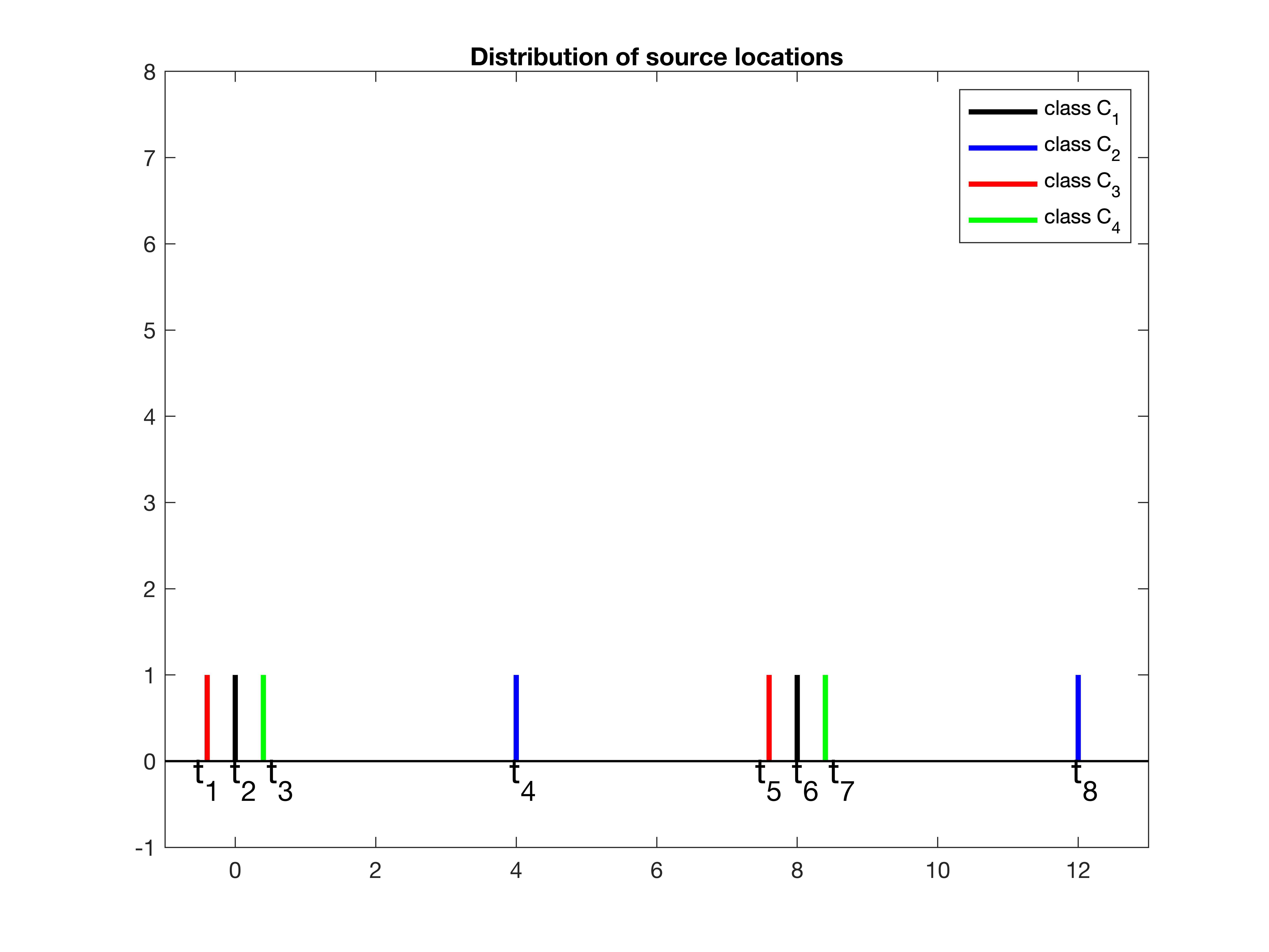
Refer to caption
Figure 8.1: Distribution of source locations.

Note that

maxj∈{1,2,…,2​n}⁡Πp∈{1,2,…,2​n},p≠j​|tp−tj|=maxk=1,2,3,4⁡(maxx∈Ck⁡Πy∈{t1,t2​…,t2​n},y≠x​|x−y|)≤maxk=1,2,3,4⁡(maxx∈Ck⁡Πp=1,2,3,4​Πy∈Cp,y≠x​|x−y|)=:maxk=1,2,3,4⁡ckmax,\begin{split}&\max_{j\in\{1,2,\dots,2n\}}\Pi_{p\in\{1,2,\dots,2n\},p\neq j}|t_{p}-t_{j}|=\max_{k=1,2,3,4}\bigg(\max_{x\in C_{k}}\Pi_{y\in\{t_{1},t_{2}\dots,t_{2n}\},y\neq x}|x-y|\bigg)\\ \leq&\max_{k=1,2,3,4}\bigg(\max_{x\in C_{k}}\Pi_{p=1,2,3,4}\Pi_{y\in C_{p},y\neq x}|x-y|\bigg)=:\max_{k=1,2,3,4}c^{\max}_{k},\end{split} (8.17)

and

minj∈{1,2,…,2​n}⁡Πp∈{1,2,…,2​n},p≠j​|tp−tj|=mink=1,2,3,4⁡(minx∈Ck⁡Πy∈{t1,t2​…,t2​n},y≠x​|x−y|)≥mink=1,2,3,4⁡(minx∈Ck⁡Πp=1,2,3,4​Πy∈Cp,y≠x​|x−y|)=:mink=1,2,3,4⁡ckmin.\begin{split}&\min_{j\in\{1,2,\dots,2n\}}\Pi_{p\in\{1,2,\dots,2n\},p\neq j}|t_{p}-t_{j}|=\min_{k=1,2,3,4}\bigg(\min_{x\in C_{k}}\Pi_{y\in\{t_{1},t_{2}\dots,t_{2n}\},y\neq x}|x-y|\bigg)\\ \geq&\min_{k=1,2,3,4}\bigg(\min_{x\in C_{k}}\Pi_{p=1,2,3,4}\Pi_{y\in C_{p},y\neq x}|x-y|\bigg)=:\min_{k=1,2,3,4}c^{\min}_{k}.\end{split} (8.18)

The estimates of maxk=1,2,3,4⁡ckmax\max_{k=1,2,3,4}c^{\max}_{k} and mink=1,2,3,4⁡ckmin\min_{k=1,2,3,4}c^{\min}_{k} are detailed in Lemmas A.3 and A.4 in Appendix A. With the aid of them we control the left-hand side of (8.16) that

Π2≤q≤2​n−1​|tj1−tjq||tj2​n−tjq|≤τ2​n−1​s2​n−1​(2​⌈n2⌉)!​(2​⌈n2⌉−1)!τ2​n−1​s2​n−3⋅((2​⌊⌊n2⌋2⌋−1)!)4≤s2​e11π2​(n+1)10​22​n−8,\begin{split}&\quad\Pi_{2\leq q\leq 2n-1}\frac{|t_{j_{1}}-t_{j_{q}}|}{|t_{j_{2n}}-t_{j_{q}}|}\leq\frac{\tau^{2n-1}s^{2n-1}\left(2\lceil\frac{n}{2}\rceil\right)!\left(2\lceil\frac{n}{2}\rceil-1\right)!}{\tau^{2n-1}s^{2n-3}\cdot\bigg((2\lfloor\frac{\lfloor\frac{n}{2}\rfloor}{2}\rfloor-1)!\bigg)^{4}}\leq\frac{s^{2}e^{11}}{\pi^{2}}(n+1)^{10}2^{2n-8},\end{split} (8.19)

where the last inequality is obtained by Lemma 8.2 in the following step.
Step 3.

Lemma 8.2.

For n≥2n\geq 2, we have

(2​⌈n2⌉)!​(2​⌈n2⌉−1)!((2​⌊⌊n2⌋2⌋−1)!)4≤e11π2​(n+1)10​22​n−8.\displaystyle\frac{\left(2\lceil\frac{n}{2}\rceil\right)!\left(2\lceil\frac{n}{2}\rceil-1\right)!}{\bigg((2\lfloor\frac{\lfloor\frac{n}{2}\rfloor}{2}\rfloor-1)!\bigg)^{4}}\leq\frac{e^{11}}{\pi^{2}}(n+1)^{10}2^{2n-8}.
Proof.

Recall the Stirling approximation of factorial, that is,

2​π​nn+12​e−n≤n!≤e​nn+12​e−n.\sqrt{2\pi}n^{n+\frac{1}{2}}e^{-n}\leq n!\leq en^{n+\frac{1}{2}}e^{-n}. (8.20)

For n≤11n\leq 11, the inequality can be checked by calculation. For n>11n>11, we have

(2​⌈n2⌉)!​(2​⌈n2⌉−1)!((2​⌊⌊n2⌋2⌋−1)!)4≤e2−4​⌈n2⌉+1​(2​⌈n2⌉)2​⌈n2⌉+12⋅(2​⌈n2⌉−1)2​⌈n2⌉−12(2​π)4​(2​⌊⌊n2⌋2⌋−1)4​(2​⌊⌊n2⌋2⌋−1)+2​e−4​(2​⌊⌊n2⌋2⌋−1)\displaystyle\frac{\left(2\lceil\frac{n}{2}\rceil\right)!\left(2\lceil\frac{n}{2}\rceil-1\right)!}{\bigg((2\lfloor\frac{\lfloor\frac{n}{2}\rfloor}{2}\rfloor-1)!\bigg)^{4}}\leq\frac{e^{2-4\lceil\frac{n}{2}\rceil+1}(2\lceil\frac{n}{2}\rceil)^{2\lceil\frac{n}{2}\rceil+\frac{1}{2}}\cdot(2\lceil\frac{n}{2}\rceil-1)^{2\lceil\frac{n}{2}\rceil-\frac{1}{2}}}{(\sqrt{2\pi})^{4}(2\lfloor\frac{\lfloor\frac{n}{2}\rfloor}{2}\rfloor-1)^{4(2\lfloor\frac{\lfloor\frac{n}{2}\rfloor}{2}\rfloor-1)+2}e^{-4(2\lfloor\frac{\lfloor\frac{n}{2}\rfloor}{2}\rfloor-1)}}
≤\displaystyle\leq 14​π2​e3−2​ne−4​(2⋅n4−1)⋅(2​(n2+12))2​n+2(2​(n4−34)−1)4​(2​(n4−34)−1)+2=14​e​π2​(n+1)2​n+2(n2−52)2​n−8\displaystyle\frac{1}{4\pi^{2}}\frac{e^{3-2n}}{e^{-4(2\cdot\frac{n}{4}-1)}}\cdot\frac{(2(\frac{n}{2}+\frac{1}{2}))^{2n+2}}{(2(\frac{n}{4}-\frac{3}{4})-1)^{4(2(\frac{n}{4}-\frac{3}{4})-1)+2}}=\frac{1}{4e\pi^{2}}\frac{(n+1)^{2n+2}}{(\frac{n}{2}-\frac{5}{2})^{2n-8}}
=\displaystyle= 14​e​π2​(n+1)10​(2+6n2−52)2​n−8=14​e​π2​(n+1)10​22​n−8​(1+6n−5)12⋅n−56+2\displaystyle\frac{1}{4e\pi^{2}}(n+1)^{10}\left(2+\frac{6}{\frac{n}{2}-\frac{5}{2}}\right)^{2n-8}=\frac{1}{4e\pi^{2}}(n+1)^{10}2^{2n-8}\left(1+\frac{6}{n-5}\right)^{12\cdot\frac{n-5}{6}+2}
≤\displaystyle\leq e114​π2​(1+6n−5)2​(n+1)10​22​n−8≤e11π2​(n+1)10​22​n−8.\displaystyle\frac{e^{11}}{4\pi^{2}}\left(1+\frac{6}{n-5}\right)^{2}(n+1)^{10}2^{2n-8}\leq\frac{e^{11}}{\pi^{2}}(n+1)^{10}2^{2n-8}.

∎

Step 4. Thus, combined (8.15) and (8.19), we have

|aj2​n|≤e11​s2π2​(n+1)10​22​n−8​|aj1|,\left|{a_{j_{2n}}}\right|\leq\frac{e^{11}s^{2}}{\pi^{2}}(n+1)^{10}2^{2n-8}\left|{a_{j_{1}}}\right|,

and consequently,

∑j=12​n|aj|≤∑q=12​n|ajq|≤2​n​e11​s2π2​(n+1)10​22​n−8​mmin.\sum_{j=1}^{2n}|a_{j}|\leq\sum_{q=1}^{2n}|a_{j_{q}}|\leq 2n\frac{e^{11}s^{2}}{\pi^{2}}(n+1)^{10}2^{2n-8}m_{\min}. (8.21)

It then follows that for k≥2​n−1k\geq 2n-1,

|∑j=12​n−1aj​tjk|≤∑j=12​n−1|aj|​(s​n2​τ)k≤\displaystyle\left|\sum_{j=1}^{2n-1}a_{j}t_{j}^{k}\right|\leq\sum_{j=1}^{2n-1}|a_{j}|\left(\frac{sn}{2}\tau\right)^{k}\leq 2​n​(n+1)10​e11​s2π2​22​n−8​mmin​(s​n2​τ)k.\displaystyle\frac{2n(n+1)^{10}e^{11}s^{2}}{\pi^{2}}2^{2n-8}m_{\min}\left(\frac{sn}{2}\tau\right)^{k}.

Step 5. We now prove that

‖ℱ⁡[μ^]−ℱ⁡[μ]‖∞≤maxx∈[−Ω,Ω]|ℱ⁡[γ]​(x)|<σ,||\mathcal{F}[\hat{\mu}]-\mathcal{F}[\mu]||_{\infty}\leq\max_{x\in[-\Omega,\Omega]}|\mathcal{F}[\gamma](x)|<\sigma,

where γ=∑j=12​naj​δtj\gamma=\sum_{j=1}^{2n}a_{j}\delta_{t_{j}}. On the other hand, similar to expansion (8.8), we can expand ℱ⁡[γ]\mathcal{F}[\gamma] and have

Qk(γ)=0,k=0,⋯,2n−2and|Qk(γ)|≤2​n​(n+1)10​e11​s2​22​n−8π2mmin(s​n2τ)k,k≥2n−1.\displaystyle Q_{k}(\gamma)=0,\ k=0,\cdots,2n-2\quad\text{and}\ |Q_{k}(\gamma)|\leq\frac{2n(n+1)^{10}e^{11}s^{2}2^{2n-8}}{\pi^{2}}m_{\min}\left(\frac{sn}{2}\tau\right)^{k},\quad k\geq 2n-1.

Therefore, for |x|≤Ω|x|\leq\Omega and n≥6n\geq 6, we have

|ℱ​[γ]​(x)|≤\displaystyle|\mathcal{F}[\gamma](x)|\leq ∑k≥2​n−12​n​(n+1)10​e11​s2π2​22​n−8​mmin​(s​n2​τ)k​|x|kk!\displaystyle\sum_{k\geq 2n-1}\frac{2n(n+1)^{10}e^{11}s^{2}}{\pi^{2}}2^{2n-8}m_{\min}\left(\frac{sn}{2}\tau\right)^{k}\frac{|x|^{k}}{k!}
≤\displaystyle\leq ∑k≥2​n−12​n​(n+1)10​e11​s2π2​22​n−8​mmin​(s​n2​τ)k​Ωkk!\displaystyle\sum_{k\geq 2n-1}\frac{2n(n+1)^{10}e^{11}s^{2}}{\pi^{2}}2^{2n-8}m_{\min}\left(\frac{sn}{2}\tau\right)^{k}\frac{\Omega^{k}}{k!}
≤\displaystyle\leq 2​e11π2⋅s2​n​(n+1)10​22​n−8​mmin⋅(s​n​τ​Ω2)2​n−1(2​n−1)!∑k=0+∞(s​τ​Ω2)k​(2​n−1)!​nk(k+2​n−1)!\displaystyle\frac{2e^{11}}{\pi^{2}}\cdot\frac{s^{2}n(n+1)^{10}2^{2n-8}m_{\min}\cdot(\frac{sn\tau\Omega}{2})^{2n-1}}{(2n-1)!}\sum_{k=0}^{+\infty}\frac{(\frac{s\tau\Omega}{2})^{k}(2n-1)!n^{k}}{(k+2n-1)!}
<\displaystyle< e1126​π2⋅(τ​Ω)2​n−1​s2​n+1​mmin​n​(n+1)10​n2​n−1(2​n−1)!⋅∑k=0+∞(s​τ​Ω2)k\displaystyle\frac{e^{11}}{2^{6}\pi^{2}}\cdot\frac{(\tau\Omega)^{2n-1}s^{2n+1}m_{\min}n(n+1)^{10}n^{2n-1}}{(2n-1)!}\cdot\sum_{k=0}^{+\infty}\left(\frac{s\tau\Omega}{2}\right)^{k}
≤\displaystyle\leq e1126​π2​(τ​Ω)2​n−1​s2​n+1​mmin​(n+1)10​n2​n​e2​n−12​π​(2​n−1)2​n−12​∑k=0+∞(s​τ​Ω2)k(by Stirling’s formula (8.2))\displaystyle\frac{e^{11}}{2^{6}\pi^{2}}(\tau\Omega)^{2n-1}s^{2n+1}m_{\min}\frac{(n+1)^{10}n^{2n}e^{2n-1}}{\sqrt{2\pi}(2n-1)^{2n-\frac{1}{2}}}\sum_{k=0}^{+\infty}\left(\frac{s\tau\Omega}{2}\right)^{k}\quad\Big(\text{by Stirling's formula (\ref{stirlingformula0})}\Big)
≤\displaystyle\leq 38⋅0.22​n−1σ⋅n​(n+1)102​n−1n2​n−1(2​n−1)2​n−1∑k=0+∞(s​τ​Ω2)k(by separation condition (2.5))\displaystyle 38\cdot 0.2^{2n-1}\sigma\cdot\frac{n(n+1)^{10}}{\sqrt{2n-1}}\frac{n^{2n-1}}{(2n-1)^{2n-1}}\sum_{k=0}^{+\infty}\left(\frac{s\tau\Omega}{2}\right)^{k}\quad\Big(\text{by separation condition (\ref{supportlowerboundequ1})}\Big)
=\displaystyle= 38⋅0.12​n−1​σ⋅n​(n+1)102​n−1​(nn−12)2​n−1​11−0.04((2.5) implies s​τ​Ω2≤0.04)\displaystyle 38\cdot 0.1^{2n-1}\sigma\cdot\frac{n(n+1)^{10}}{\sqrt{2n-1}}\left(\frac{n}{n-\frac{1}{2}}\right)^{2n-1}\frac{1}{1-0.04}\quad\Big(\text{(\ref{supportlowerboundequ1}) implies $\frac{s\tau\Omega}{2}\leq 0.04$}\Big)
≤\displaystyle\leq 38​e⋅0.12​n−1​σ⋅n​(n+1)102​n−1​11−0.04\displaystyle 38e\cdot 0.1^{2n-1}\sigma\cdot\frac{n(n+1)^{10}}{\sqrt{2n-1}}\frac{1}{1-0.04}
<\displaystyle< σ(38​e⋅0.12​n−1⋅n​(n+1)102​n−1​11−0.04<1 for n≥6).\displaystyle\sigma\quad\left(\text{$38e\cdot 0.1^{2n-1}\cdot\frac{n(n+1)^{10}}{\sqrt{2n-1}}\frac{1}{1-0.04}<1$ for $n\geq 6$}\right).

It then follows that ‖ℱ⁡[μ^]−ℱ⁡[μ]‖∞<σ||\mathcal{F}[\hat{\mu}]-\mathcal{F}[\mu]||_{\infty}<\sigma.

Now consider the case when 2≤n≤52\leq n\leq 5. By (8.19), we have

Π2≤q≤2​n−1​|tj1−tjq||tj2​n−tjq|≤s2​(2​⌈n2⌉)!​(2​⌈n2⌉−1)!((2​⌊⌊n2⌋2⌋−1)!)4,\Pi_{2\leq q\leq 2n-1}\frac{|t_{j_{1}}-t_{j_{q}}|}{|t_{j_{2n}}-t_{j_{q}}|}\leq\frac{s^{2}\left(2\lceil\frac{n}{2}\rceil\right)!\left(2\lceil\frac{n}{2}\rceil-1\right)!}{\bigg((2\lfloor\frac{\lfloor\frac{n}{2}\rfloor}{2}\rfloor-1)!\bigg)^{4}},

and consequently,

∑j=12​n|aj|≤2​n​s2​(2​⌈n2⌉)!​(2​⌈n2⌉−1)!((2​⌊⌊n2⌋2⌋−1)!)4.\sum_{j=1}^{2n}|a_{j}|\leq 2n\frac{s^{2}\left(2\lceil\frac{n}{2}\rceil\right)!\left(2\lceil\frac{n}{2}\rceil-1\right)!}{\bigg((2\lfloor\frac{\lfloor\frac{n}{2}\rfloor}{2}\rfloor-1)!\bigg)^{4}}.

By similar arguments as those for the case when n≥6n\geq 6, we can show that for 2≤n≤52\leq n\leq 5,

|ℱ​[γ]​(x)|<σ.|\mathcal{F}[\gamma](x)|<\sigma.

∎

9 Proof of results in Section 4

9.1 Proof of Theorem 4.1

Proof.

Step 1. We first prove the one-dimensional case. Let μ=∑j=12aj​δyj,aj=mmin​ei​θj\mu=\sum_{j=1}^{2}a_{j}\delta_{y_{j}},a_{j}=m_{\min}e^{i\theta_{j}} and μ^=a​δy^\hat{\mu}=a\delta_{\hat{y}}. A crucial relation is

ℱ⁡[μ^]​(ω)=ℱ⁡[μ]​(ω)+𝐰1​(ω),|𝐰1​(ω)|<2​σ,ω∈[−Ω,Ω].\mathcal{F}[\hat{\mu}](\omega)=\mathcal{F}[\mu](\omega)+\boldsymbol{\mathbf{w}}_{1}(\omega),\ |\boldsymbol{\mathbf{w}}_{1}(\omega)|<2\sigma,\ \omega\in[-\Omega,\Omega]. (9.1)

Note that if (9.1) holds, μ^\hat{\mu} can be a σ\sigma-admissible measure of some 𝐘\boldsymbol{\mathbf{Y}} generated by model (3.2). This time, resolving two point sources is impossible. Conversely, if (9.1) does not hold, μ^\hat{\mu} cannot be any σ\sigma-admissible measure of some 𝐘\boldsymbol{\mathbf{Y}} generated by μ\mu as in model (3.2). Thus the resolution limit ℛ⁡(θ)\mathcal{R}(\theta) is the constant such that (9.1) holds when |y1−y2|<ℛ⁡(θ)|y_{1}-y_{2}|<\mathcal{R}(\theta) and fails to hold in the opposite case.

Step 2. Note that for the general source locations y1,y2y_{1},y_{2}, shifting them by xx and get that

ℱ⁡[μ^]​(ω)​ei​x​ω=ℱ⁡[μ]​(ω)​ei​x​ω+𝐰1​(ω)​ei​x​ω,|𝐰1​(ω)​ei​x​ω|<2​σ,ω∈[−Ω,Ω],\mathcal{F}[\hat{\mu}](\omega)e^{ix\omega}=\mathcal{F}[\mu](\omega)e^{ix\omega}+\boldsymbol{\mathbf{w}}_{1}(\omega)e^{ix\omega},\ |\boldsymbol{\mathbf{w}}_{1}(\omega)e^{ix\omega}|<2\sigma,\ \omega\in[-\Omega,\Omega],

we can transform the problem into the case when y1=−y2y_{1}=-y_{2}. Thus we consider that the underlying source is μ=mmin​ei​θ2​δy1+mmin​ei​−θ2​δy2\mu=m_{\min}e^{i\frac{\theta}{2}}\delta_{y_{1}}+m_{\min}e^{i\frac{-\theta}{2}}\delta_{y_{2}} with y1>0,y1=−y2y_{1}>0,y_{1}=-y_{2}. The measure μ^\hat{\mu} is a​δy^a\delta_{\hat{y}} with aa and y^\hat{y} to be determined.

From (9.1), we get that

𝐰1​(ω)=a​ei​y^​ω−mmin​(ei​θ2​ei​y1​ω+ei​−θ2​ei​y2​ω)=a​ei​y^​ω−2​mmin​cos⁡(y1​ω+θ2).\displaystyle\boldsymbol{\mathbf{w}}_{1}(\omega)=ae^{i\hat{y}\omega}-m_{\min}(e^{i\frac{\theta}{2}}e^{iy_{1}\omega}+e^{i\frac{-\theta}{2}}e^{iy_{2}\omega})=ae^{i\hat{y}\omega}-2m_{\min}\cos\left(y_{1}\omega+\frac{\theta}{2}\right).

Note that for two non-negative values x,yx,y, we have

|x​ei​q−y|2=(x​cos⁡(q)−y)2+x2​sin2⁡(q)=x2+y2−2​x​y​cos⁡(q)≥(x−y)2\left|xe^{iq}-y\right|^{2}=(x\cos(q)-y)^{2}+x^{2}\sin^{2}(q)=x^{2}+y^{2}-2xy\cos(q)\geq(x-y)^{2} (9.2)

and the equality is attained when q=0q=0. We only consider the case when

0≤y1​Ω+θ2≤π2​ and −π2≤−y1​Ω+θ2≤00\leq y_{1}\Omega+\frac{\theta}{2}\leq\frac{\pi}{2}\text{ and }-\frac{\pi}{2}\leq-y_{1}\Omega+\frac{\theta}{2}\leq 0 (9.3)

and we shall see that this coincides with the case in the theorem. By the above condition, we have cos⁡(y1​ω+θ2)≥0,ω∈[−Ω,Ω]\cos(y_{1}\omega+\frac{\theta}{2})\geq 0,\omega\in[-\Omega,\Omega]. Thus by (9.2), for every ω\omega,

|𝐰1​(ω)|≥||a|−2​mmin​cos⁡(y1​ω+θ2)||\boldsymbol{\mathbf{w}}_{1}(\omega)|\geq\left||a|-2m_{\min}\cos\left(y_{1}\omega+\frac{\theta}{2}\right)\right|

and the minimum is attained when y^=0\hat{y}=0 and aa is a positive number. We now try to find the condition on y1y_{1} so that there exists aa satisfying

||a|−2​mmin​cos⁡(y1​ω+θ2)|<2​σ,ω∈[−Ω,Ω].\left||a|-2m_{\min}\cos\left(y_{1}\omega+\frac{\theta}{2}\right)\right|<2\sigma,\quad\omega\in[-\Omega,\Omega].

This is equivalent to

maxω,ω′∈[−Ω,Ω]⁡|2​mmin​(cos⁡(y1​ω+θ2)−cos⁡(y1​ω′+θ2))|<4​σ.\max_{\omega,\omega^{\prime}\in[-\Omega,\Omega]}\left|2m_{\min}\left(\cos\left(y_{1}\omega+\frac{\theta}{2}\right)-\cos\left(y_{1}\omega^{\prime}+\frac{\theta}{2}\right)\right)\right|<4\sigma. (9.4)

We then analyze the problem for two different cases. We denote dmin:=|y1−y2|d_{\min}:=|y_{1}-y_{2}| and now the condition (9.3) is

0≤dmin​Ω+θ2≤π2​ and ​−dmin​Ω+θ2≤0.0\leq\frac{d_{\min}\Omega+\theta}{2}\leq\frac{\pi}{2}\text{ and }\frac{-d_{\min}\Omega+\theta}{2}\leq 0. (9.5)

Under this condition, problem (9.4) becomes

2​mmin​|1−cos⁡(dmin2​Ω+θ2)|<4​σ.2m_{\min}\left|1-\cos\left(\frac{d_{\min}}{2}\Omega+\frac{\theta}{2}\right)\right|<4\sigma.

Thus 4sin(dmin​Ω+θ4)2<4​σmmin4\sin\left(\frac{d_{\min}\Omega+\theta}{4}\right)^{2}<\frac{4\sigma}{m_{\min}}, and equivalently

dmin<4​arcsin⁡((σmmin)12)−θΩ.d_{\min}<\frac{4\arcsin\left(\left(\frac{\sigma}{m_{\min}}\right)^{\frac{1}{2}}\right)-\theta}{\Omega}.

By the above discussions, in this case ℛ⁡(θ)\mathcal{R}(\theta) is

ℛ⁡(θ)=4​arcsin⁡((σmmin)12)−θΩ.\mathcal{R}(\theta)=\frac{4\arcsin\left(\left(\frac{\sigma}{m_{\min}}\right)^{\frac{1}{2}}\right)-\theta}{\Omega}.

Now the condition (9.5) holds when

4​arcsin⁡((σmmin)12)−θΩ​Ω+θ≤π,and−(4​arcsin⁡((σmmin)12)−θΩ)​Ω+θ≤0.\frac{4\arcsin\left(\left(\frac{\sigma}{m_{\min}}\right)^{\frac{1}{2}}\right)-\theta}{\Omega}\Omega+\theta\leq\pi,\text{and}-\left(\frac{4\arcsin\left(\left(\frac{\sigma}{m_{\min}}\right)^{\frac{1}{2}}\right)-\theta}{\Omega}\right)\Omega+\theta\leq 0.

which further holds when

sin⁡(θ2)2≤σmmin≤12.\sin\left(\frac{\theta}{2}\right)^{2}\leq\frac{\sigma}{m_{\min}}\leq\frac{1}{2}.

This proves the first case in the theorem.

Now, we consider the case when σmmin>12\frac{\sigma}{m_{\min}}>\frac{1}{2}. We choose the specific case where a=mmin​ei​θ1a=m_{\min}e^{i\theta_{1}} and y^=y1\hat{y}=y_{1}. Then

𝐰1​(ω)=mmin​ei​θ1​ei​y1​ω−(mmin​ei​θ1​ei​y1​ω+mmin​ei​θ2​ei​y2​ω)=mmin​ei​θ2​ei​y2​ω,ω∈[−Ω,Ω].\boldsymbol{\mathbf{w}}_{1}(\omega)=m_{\min}e^{i\theta_{1}}e^{iy_{1}\omega}-(m_{\min}e^{i\theta_{1}}e^{iy_{1}\omega}+m_{\min}e^{i\theta_{2}}e^{iy_{2}\omega})=m_{\min}e^{i\theta_{2}}e^{iy_{2}\omega},\quad\omega\in[-\Omega,\Omega].

Condition σmmin>12\frac{\sigma}{m_{\min}}>\frac{1}{2} gives

|𝐰1​(ω)|<2​σ.|\boldsymbol{\mathbf{w}}_{1}(\omega)|<2\sigma.

Thus the case when σmmin>12\frac{\sigma}{m_{\min}}>\frac{1}{2} is meaningless. Indeed, there are always some σ\sigma-admissible measures for some images with only one point source.

Step 3. Now we consider the case when the sources 𝐲j\boldsymbol{\mathbf{y}}_{j}’s are in ℝk\mathbb{R}^{k}. We still consider the crucial relation that

ℱ⁡[μ^]​(𝝎)=ℱ⁡[μ]​(𝝎)+𝐰1​(𝝎),|𝐰1​(𝝎)|<2​σ,||𝝎||2≤Ω.\mathcal{F}[\hat{\mu}](\boldsymbol{\mathbf{\omega}})=\mathcal{F}[\mu](\boldsymbol{\mathbf{\omega}})+\boldsymbol{\mathbf{w}}_{1}(\boldsymbol{\mathbf{\omega}}),\ |\boldsymbol{\mathbf{w}}_{1}(\boldsymbol{\mathbf{\omega}})|<2\sigma,\ \left|\left|{\boldsymbol{\mathbf{\omega}}}\right|\right|_{2}\leq\Omega. (9.6)

By a similar argument as the one in step 1, we know that the resolution limit ℛ⁡(θ)\mathcal{R}(\theta) is the constant such that (9.6) holds when ||𝐲1−𝐲2||2<ℛ⁡(θ)\left|\left|{\boldsymbol{\mathbf{y}}_{1}-\boldsymbol{\mathbf{y}}_{2}}\right|\right|_{2}<\mathcal{R}(\theta) and fails to hold in the opposite case. Note that by choosing suitable axes or transforming the problem, we can make 𝐲1=(y1,0,⋯,0)⊤,𝐲2=(y2,0,⋯,0)⊤\boldsymbol{\mathbf{y}}_{1}=(y_{1},0,\cdots,0)^{\top},\boldsymbol{\mathbf{y}}_{2}=(y_{2},0,\cdots,0)^{\top}. Consider μ^=a​δ𝐲^,𝐲^∈ℝk\hat{\mu}=a\delta_{\mathbf{\hat{y}}},\mathbf{\hat{y}}\in\mathbb{R}^{k} with aa and 𝐲^\mathbf{\hat{y}} to be determined. We now have

ℱ[μ^](𝝎)−ℱ[μ](𝝎)=aei​𝐲^⋅𝝎−∑j=12ajei​𝐲j⋅𝝎=aei𝐲^2:k⋅𝝎2:ke𝐲^1​𝝎1−∑j=12ajei​yj​𝝎1.\mathcal{F}[\hat{\mu}](\boldsymbol{\mathbf{\omega}})-\mathcal{F}[\mu](\boldsymbol{\mathbf{\omega}})=ae^{i\mathbf{\hat{y}}\cdot\boldsymbol{\mathbf{\omega}}}-\sum_{j=1}^{2}a_{j}e^{i\boldsymbol{\mathbf{y}}_{j}\cdot\boldsymbol{\mathbf{\omega}}}=ae^{i\mathbf{\hat{y}}_{2:k}\cdot\boldsymbol{\mathbf{\omega}}_{2:k}}e^{\mathbf{\hat{y}}_{1}\boldsymbol{\mathbf{\omega}}_{1}}-\sum_{j=1}^{2}a_{j}e^{i{y}_{j}\boldsymbol{\mathbf{\omega}}_{1}}.

Thus analyzing when (9.6) holds can be reduced to the one-dimensional case and it is not hard to see the result for the one-dimensional space still holds for multi-dimensional spaces.

∎

9.2 Proof of Theorem 4.2

Proof.

Step 1. We only need to analyze the case when σmmin≤12\frac{\sigma}{m_{\min}}\leq\frac{1}{2}, as the case when σmmin>12\frac{\sigma}{m_{\min}}>\frac{1}{2} is trivial. Also, we only consider the one-dimensional case since the treatment for multi-dimensional spaces is similar to the one in the proof of Theorem 4.1.

Similarly to step 1 in the proof of Theorem 4.1, the resolution limit 𝒟k,n​u​m\mathcal{D}_{k,num} should be the constant such that the following estimate:

ℱ⁡[μ^]​(ω)=ℱ⁡[μ]​(ω)+𝐰2​(ω),|𝐰2​(ω)|<2​σ,ω∈[−Ω,Ω],\mathcal{F}[\hat{\mu}](\omega)=\mathcal{F}[\mu](\omega)+\boldsymbol{\mathbf{w}}_{2}(\omega),\ |\boldsymbol{\mathbf{w}}_{2}(\omega)|<2\sigma,\ \omega\in[-\Omega,\Omega], (9.7)

holds when |y1−y2|<𝒟k,n​u​m|y_{1}-y_{2}|<\mathcal{D}_{k,num} and fails to hold in the opposite case. We shall prove that when sin⁡(θ2)2≤σmmin≤12\sin\left(\frac{\theta}{2}\right)^{2}\leq\frac{\sigma}{m_{\min}}\leq\frac{1}{2}, if

|y1−y2|≥4​arcsin⁡((σmmin)12)Ω,\left|y_{1}-y_{2}\right|\geq\frac{4\arcsin\left(\left(\frac{\sigma}{m_{\min}}\right)^{\frac{1}{2}}\right)}{\Omega},

then (9.7) doesn’t hold for any μ^\hat{\mu} consisting of only one source. On the opposite case, Theorem 4.1 already ensures the existence of such μ^\hat{\mu} making

|𝐰2​(ω)|<2​σ,ω∈[−Ω,Ω].\left|\mathbf{w}_{2}(\omega)\right|<2\sigma,\quad\omega\in[-\Omega,\Omega].

This is enough to prove the theorem.

Step 2. Without loss of generality, we assume the underlying source is

μ=mmin​α​e−i​β​δy1+mmin​ei​β​δy2\mu=m_{\min}\alpha e^{-i\beta}\delta_{y_{1}}+m_{\min}e^{i\beta}\delta_{y_{2}}

with y1=−y2y_{1}=-y_{2}, 0<y1≤π2​Ω0<y_{1}\leq\frac{\pi}{2\Omega}, α≥1\alpha\geq 1 and 0≤β≤π40\leq\beta\leq\frac{\pi}{4}. It is not hard to see that the other cases can all be transformed to the above setting or the same analysis as follows can be applied to. We consider μ^=a​ei​γ​δy^\hat{\mu}=ae^{i\gamma}\delta_{\hat{y}} with a>0a>0, γ\gamma and y^\hat{y} to be determined.

From (9.7), we have

𝐰2​(ω)\displaystyle\boldsymbol{\mathbf{w}}_{2}(\omega) =a​ei​γ​ei​y^​ω−mmin​(α​e−i​β​ei​y1​ω+ei​β​e−i​y1​ω).\displaystyle=ae^{i\gamma}e^{i\hat{y}\omega}-m_{\min}\left(\alpha e^{-i\beta}e^{iy_{1}\omega}+e^{i\beta}e^{-iy_{1}\omega}\right).

We rewrite it as

𝐰2​(ω)=\displaystyle\boldsymbol{\mathbf{w}}_{2}(\omega)= a​ei​γ​ei​y^​ω−mmin​(α​ei⁡(y1​ω−β)+ei⁡(β−y1​ω)).\displaystyle ae^{i\gamma}e^{i\hat{y}\omega}-m_{\min}\left(\alpha e^{i(y_{1}\omega-\beta)}+e^{i(\beta-y_{1}\omega)}\right).
=\displaystyle= a​ei​γ​ei​y^​ω−h​mmin​ei⁡(y1​ω−β)−2​mmin​cos⁡(y1​ω−β)\displaystyle ae^{i\gamma}e^{i\hat{y}\omega}-hm_{\min}e^{i(y_{1}\omega-\beta)}-2m_{\min}\cos(y_{1}\omega-\beta) (9.8)

where α=mmin​(1+h)\alpha=m_{\min}(1+h). We next prove the theorem by considering the case when

y1​Ω≥β,0≤Ω​y1+β≤π2.y_{1}\Omega\geq\beta,\quad 0\leq\Omega y_{1}+\beta\leq\frac{\pi}{2}. (9.9)

We consider the necessary condition for the existence of such μ^,μ\hat{\mu},\mu satisfying (9.7) that

mina>0,α≥1,γ∈ℝ,y^∈ℝ⁡|𝐰2​(−Ω)|+|𝐰2​(βy1)|<4​σ.\min_{a>0,\alpha\geq 1,\gamma\in\mathbb{R},\hat{y}\in\mathbb{R}}\left|{\boldsymbol{\mathbf{w}}_{2}(-\Omega)}\right|+\left|{\boldsymbol{\mathbf{w}}_{2}(\frac{\beta}{y_{1}})}\right|<4\sigma.

By (9.2), it is

mina>0,h≥0,γ∈ℝ,y^∈ℝ⁡|a​ei​γ​e−i​y^​Ω−h​mmin​e−i⁡(y1​Ω+β)−2​mmin​cos⁡(y1​Ω+β)|+|a​ei​γ​ei​y^​βy1−(2​mmin+h​mmin)|.\displaystyle\min_{a>0,h\geq 0,\gamma\in\mathbb{R},\hat{y}\in\mathbb{R}}\left|ae^{i\gamma}e^{-i\hat{y}\Omega}-hm_{\min}e^{-i(y_{1}\Omega+\beta)}-2m_{\min}\cos(y_{1}\Omega+\beta)\right|+\left|ae^{i\gamma}e^{i\hat{y}\frac{\beta}{y_{1}}}-(2m_{\min}+hm_{\min})\right|. (9.10)

A key observation is that if 2​mmin​cos⁡(y1​Ω+β)+h​mmin≤a≤2​mmin+h​mmin2m_{\min}\cos(y_{1}\Omega+\beta)+hm_{\min}\leq a\leq 2m_{\min}+hm_{\min}, we have

mina>0,h≥0,γ∈ℝ,y^∈ℝ⁡|a​ei​γ​e−i​y^​Ω−h​mmin​e−i⁡(y1​Ω+β)−2​mmin​cos⁡(y1​Ω+β)|+|a​ei​γ​ei​y^​βy1−(2​mmin+h​mmin)|\displaystyle\min_{a>0,h\geq 0,\gamma\in\mathbb{R},\hat{y}\in\mathbb{R}}\left|ae^{i\gamma}e^{-i\hat{y}\Omega}-hm_{\min}e^{-i(y_{1}\Omega+\beta)}-2m_{\min}\cos(y_{1}\Omega+\beta)\right|+\left|ae^{i\gamma}e^{i\hat{y}\frac{\beta}{y_{1}}}-(2m_{\min}+hm_{\min})\right|
≥\displaystyle\geq mina>0,h≥0,γ∈ℝ,y^∈ℝ,x^∈ℝ⁡|a​e−i​y^​Ω−h​mmin​e−i​x^​Ω−2​mmin​cos⁡(y1​Ω+β)|+|a​ei​γ−(2​mmin+h​mmin)|\displaystyle\min_{a>0,h\geq 0,\gamma\in\mathbb{R},\hat{y}\in\mathbb{R},\hat{x}\in\mathbb{R}}\left|ae^{-i\hat{y}\Omega}-hm_{\min}e^{-i\hat{x}\Omega}-2m_{\min}\cos(y_{1}\Omega+\beta)\right|+|ae^{i\gamma}-(2m_{\min}+hm_{\min})|
=\displaystyle= mina>0,h≥0⁡|a−h​mmin−2​mmin​cos⁡(y1​Ω+β)|+|a−(2​mmin+h​mmin)|\displaystyle\min_{a>0,h\geq 0}\left|a-hm_{\min}-2m_{\min}\cos(y_{1}\Omega+\beta)\right|+\left|a-(2m_{\min}+hm_{\min})\right|
=\displaystyle= minb∈ℝ, 2​mmin​cos⁡(y1​Ω+β)≤b≤2​mmin⁡|b−2​mmin​cos⁡(y1​Ω+β)|+|2​mmin−b|\displaystyle\min_{b\in\mathbb{R},\ 2m_{\min}\cos(y_{1}\Omega+\beta)\leq b\leq 2m_{\min}}\left|b-2m_{\min}\cos(y_{1}\Omega+\beta)\right|+|2m_{\min}-b|
=\displaystyle= 2​mmin−2​mmin​cos⁡(y1​Ω+β),\displaystyle 2m_{\min}-2m_{\min}\cos(y_{1}\Omega+\beta), (9.11)

where the first equality is because 2​mmin​cos⁡(y1​Ω)+h​mmin≤a≤2​mmin+h​mmin2m_{\min}\cos(y_{1}\Omega)+hm_{\min}\leq a\leq 2m_{\min}+hm_{\min} and 2​mmin​cos⁡(y1​Ω+β)≥02m_{\min}\cos(y_{1}\Omega+\beta)\geq 0 by (9.9).

On the other hand, letting h=0,y^=0,γ=0h=0,\hat{y}=0,\gamma=0, we have

mina>0⁡|a​ei​γ​e−i​y^​Ω−h​mmin​e−i⁡(y1​Ω+β)−2​mmin​cos⁡(y1​Ω+β)|+|a​ei​γ​ei​y^​βy1−(2​mmin+h​mmin)|.\displaystyle\min_{a>0}\left|ae^{i\gamma}e^{-i\hat{y}\Omega}-hm_{\min}e^{-i(y_{1}\Omega+\beta)}-2m_{\min}\cos(y_{1}\Omega+\beta)\right|+\left|ae^{i\gamma}e^{i\hat{y}\frac{\beta}{y_{1}}}-(2m_{\min}+hm_{\min})\right|.
=\displaystyle= mina>0⁡|a−2​mmin​cos⁡(y1​Ω+β)|+|a−2​mmin|\displaystyle\min_{a>0}\left|a-2m_{\min}\cos(y_{1}\Omega+\beta)\right|+|a-2m_{\min}|
=\displaystyle= mina>0⁡(a−2​mmin​cos⁡(y1​Ω+β))+2​mmin−a(choose 2​mmin​cos⁡(y1​Ω+β)≤a≤2​mmin)\displaystyle\min_{a>0}(a-2m_{\min}\cos(y_{1}\Omega+\beta))+2m_{\min}-a\quad\big(\text{choose $2m_{\min}\cos(y_{1}\Omega+\beta)\leq a\leq 2m_{\min}$}\big)
=\displaystyle= 2​mmin−2​mmin​cos⁡(y1​Ω+β).\displaystyle 2m_{\min}-2m_{\min}\cos(y_{1}\Omega+\beta).

Together with (9.11), this yields

mina>0,h≥0,γ∈ℝ,y^∈ℝ⁡|a​ei​γ​e−i​y^​Ω−h​mmin​e−i⁡(y1​Ω+β)−2​mmin​cos⁡(y1​Ω+β)|+|a​ei​γ​ei​y^​βy1−(2​mmin+h​mmin)|\displaystyle\min_{a>0,h\geq 0,\gamma\in\mathbb{R},\hat{y}\in\mathbb{R}}\left|ae^{i\gamma}e^{-i\hat{y}\Omega}-hm_{\min}e^{-i(y_{1}\Omega+\beta)}-2m_{\min}\cos(y_{1}\Omega+\beta)\right|+\left|ae^{i\gamma}e^{i\hat{y}\frac{\beta}{y_{1}}}-(2m_{\min}+hm_{\min})\right|
=\displaystyle= 2​mmin−2​mmin​cos⁡(y1​Ω+β),\displaystyle 2m_{\min}-2m_{\min}\cos(y_{1}\Omega+\beta),

in the case when 2​mmin​cos⁡(y1​Ω+β)+h​mmin≤a≤2​mmin+h​mmin2m_{\min}\cos(y_{1}\Omega+\beta)+hm_{\min}\leq a\leq 2m_{\min}+hm_{\min}.

Now, we consider the case when a<2​mmin​cos⁡(y1​Ω+β)+h​mmina<2m_{\min}\cos(y_{1}\Omega+\beta)+hm_{\min}. In this case, we have

mina>0,h≥0,γ∈ℝ,y^∈ℝ⁡|a​ei​γ​e−i​y^​Ω−h​mmin​e−i⁡(y1​Ω+β)−2​mmin​cos⁡(y1​Ω+β)|+|a​ei​γ​ei​y^​βy1−(2​mmin+h​mmin)|\displaystyle\min_{a>0,h\geq 0,\gamma\in\mathbb{R},\hat{y}\in\mathbb{R}}\left|ae^{i\gamma}e^{-i\hat{y}\Omega}-hm_{\min}e^{-i(y_{1}\Omega+\beta)}-2m_{\min}\cos(y_{1}\Omega+\beta)\right|+\left|ae^{i\gamma}e^{i\hat{y}\frac{\beta}{y_{1}}}-(2m_{\min}+hm_{\min})\right|
≥\displaystyle\geq mina>0,h≥0,γ∈ℝ,a<2​mmin​cos⁡(y1​Ω+β)+h​mmin⁡|a​ei​γ−(2​mmin+h​mmin)|\displaystyle\min_{a>0,h\geq 0,\gamma\in\mathbb{R},a<2m_{\min}\cos(y_{1}\Omega+\beta)+hm_{\min}}\left|{ae^{i\gamma}-(2m_{\min}+hm_{\min})}\right|
≥\displaystyle\geq mina>0,h≥0,a<2​mmin​cos⁡(y1​Ω+β)+h​mmin⁡|a−(2​mmin+h​mmin)|\displaystyle\min_{a>0,h\geq 0,a<2m_{\min}\cos(y_{1}\Omega+\beta)+hm_{\min}}\left|{a-(2m_{\min}+hm_{\min})}\right|
=\displaystyle= mina>0,h≥0,a<2​mmin​cos⁡(y1​Ω+β)+h​mmin⁡2​mmin+h​mmin−a\displaystyle\min_{a>0,h\geq 0,a<2m_{\min}\cos(y_{1}\Omega+\beta)+hm_{\min}}2m_{\min}+hm_{\min}-a
>\displaystyle> 2​mmin−2​mmin​cos⁡(y1​Ω+β).\displaystyle 2m_{\min}-2m_{\min}\cos(y_{1}\Omega+\beta).

Finally, we consider the case when a>2​mmin+h​mmina>2m_{\min}+hm_{\min}. In this case, we have

mina>0,h≥0,γ∈ℝ,y^∈ℝ⁡|a​ei​γ​e−i​y^​Ω−h​mmin​e−i​y1​Ω−2​mmin​cos⁡(y1​Ω+β)|+|a​ei​γ​ei​y^​βy1−(2​mmin+h​mmin)|\displaystyle\min_{a>0,h\geq 0,\gamma\in\mathbb{R},\hat{y}\in\mathbb{R}}\left|ae^{i\gamma}e^{-i\hat{y}\Omega}-hm_{\min}e^{-iy_{1}\Omega}-2m_{\min}\cos(y_{1}\Omega+\beta)\right|+\left|ae^{i\gamma}e^{i\hat{y}\frac{\beta}{y_{1}}}-(2m_{\min}+hm_{\min})\right|
≥\displaystyle\geq mina>0,h≥0,γ∈ℝ,y^∈ℝ,a>2​mmin+h​mmin⁡|a​ei​γ​e−i​y^​Ω−h​mmin​e−i​y1​Ω−2​mmin​cos⁡(y1​Ω+β)|\displaystyle\min_{a>0,h\geq 0,\gamma\in\mathbb{R},\hat{y}\in\mathbb{R},a>2m_{\min}+hm_{\min}}\left|ae^{i\gamma}e^{-i\hat{y}\Omega}-hm_{\min}e^{-iy_{1}\Omega}-2m_{\min}\cos(y_{1}\Omega+\beta)\right|
≥\displaystyle\geq mina>0,h≥0,a>2​mmin+h​mmin⁡a−(2​mmin​cos⁡(y1​Ω+β)+h​mmin)\displaystyle\min_{a>0,h\geq 0,a>2m_{\min}+hm_{\min}}a-(2m_{\min}\cos(y_{1}\Omega+\beta)+hm_{\min})
>\displaystyle> 2​mmin−2​mmin​cos⁡(y1​Ω+β).\displaystyle 2m_{\min}-2m_{\min}\cos(y_{1}\Omega+\beta).

Therefore, combining all the above discussions, we arrive at

mina>0,h≥0,γ∈ℝ,y^∈ℝ⁡|a​ei​γ​e−i​y^​Ω−h​mmin​e−i​y1​Ω−2​mmin​cos⁡(y1​Ω+β)|+|a​ei​γ​ei​y^​βy1−(2​mmin+h​mmin)|\displaystyle\min_{a>0,h\geq 0,\gamma\in\mathbb{R},\hat{y}\in\mathbb{R}}\left|ae^{i\gamma}e^{-i\hat{y}\Omega}-hm_{\min}e^{-iy_{1}\Omega}-2m_{\min}\cos(y_{1}\Omega+\beta)\right|+\left|ae^{i\gamma}e^{i\hat{y}\frac{\beta}{y_{1}}}-(2m_{\min}+hm_{\min})\right|
=\displaystyle= 2​mmin−2​mmin​cos⁡(y1​Ω+β).\displaystyle 2m_{\min}-2m_{\min}\cos(y_{1}\Omega+\beta).

Thus (9.10) is equivalent to

2​mmin−2​mmin​cos⁡(y1​Ω+β)<4​σ.2m_{\min}-2m_{\min}\cos(y_{1}\Omega+\beta)<4\sigma.

Similar to the proof of Theorem 4.1, this yields

dmin<4​arcsin⁡((σmmin)12)−θΩ.d_{\min}<\frac{4\arcsin\left(\left(\frac{\sigma}{m_{\min}}\right)^{\frac{1}{2}}\right)-\theta}{\Omega}.

where θ=2​β\theta=2\beta in our setting. The condition (9.9) now holds when

sin⁡(θ2)2≤σmmin≤12.\sin\left(\frac{\theta}{2}\right)^{2}\leq\frac{\sigma}{m_{\min}}\leq\frac{1}{2}.

This completes the proof.

∎

Appendix A Auxiliary lemmas

The following results can be easily proved.

Lemma A.1.

Let n∈ℕ+n\in\mathbb{N}^{+} and τ>0\tau>0 and let 𝒞={j=1,2,…,n}\mathcal{C}=\{j=1,2,\dots,n\}. Then

(1):

⌈n2⌉∈arg⁡minz∈𝒞​Πx∈𝒞,x≠z​|x−z|,\lceil\frac{n}{2}\rceil\in\arg\min_{z\in\mathcal{C}}\Pi_{x\in\mathcal{C},x\neq z}|x-z|, (A.1)

and

minz∈𝒞⁡Πx∈𝒞,x≠z​|x−z|=(⌈n2⌉−1)!​(⌊n2⌋)!;\min_{z\in\mathcal{C}}\Pi_{x\in\mathcal{C},x\neq z}|x-z|=\left(\lceil\frac{n}{2}\rceil-1\right)!\left(\lfloor\frac{n}{2}\rfloor\right)!; (A.2)

(2):

arg⁡maxz∈𝒞​Πx∈𝒞,x≠z​|x−z|={1,n},\arg\max_{z\in\mathcal{C}}\Pi_{x\in\mathcal{C},x\neq z}|x-z|=\{1,n\}, (A.3)

and

maxz∈𝒞⁡Πx∈𝒞,x≠z​|x−z|=(n−1)!.\max_{z\in\mathcal{C}}\Pi_{x\in\mathcal{C},x\neq z}|x-z|=(n-1)!. (A.4)
Lemma A.2.

Let n∈ℕ+n\in\mathbb{N}^{+} and let p,q∈ℝp,q\in\mathbb{R} be such that p>q>0p>q>0. For the following three sets of evenly spaced points 𝒞1:={xj=(j−1)​p,j=1,…,n}\mathcal{C}_{1}:=\{x_{j}=(j-1)p,j=1,\dots,n\}, 𝒞2:={yj=(j−1)​p−q,j=1,…,n}\mathcal{C}_{2}:=\{y_{j}=(j-1)p-q,j=1,\dots,n\}, and 𝒞3:={yj=(j−1)​p−q,j=1,…,n+1}\mathcal{C}_{3}:=\{y_{j}=(j-1)p-q,j=1,\dots,n+1\}, we have
(1): arg⁡minz∈𝒞2​Πj=1n​|z−xj|⊂{y⌊n2⌋+1,y⌊n2⌋+2}\arg\min_{z\in\mathcal{C}_{2}}\Pi_{j=1}^{n}|z-x_{j}|\subset\{y_{\lfloor\frac{n}{2}\rfloor+1},y_{\lfloor\frac{n}{2}\rfloor+2}\}, and

minz∈𝒞2⁡Πi=1n|z−xi|=Πj=0⌈n2⌉−1​(min⁡(p−q,q)+p​j)⋅Πj=0⌊n2⌋−1​(max⁡(p−q,q)+p​j);\min_{z\in\mathcal{C}_{2}}\Pi_{i=1}^{n}|z-x_{i}|=\Pi_{j=0}^{\lceil\frac{n}{2}\rceil-1}\left(\min(p-q,q)+pj\right)\cdot\Pi_{j=0}^{\lfloor\frac{n}{2}\rfloor-1}\left(\max(p-q,q)+pj\right); (A.5)

(2): arg⁡minz∈𝒞3​Πj=1n​|z−xj|⊂{y⌊n2⌋+1,y⌊n2⌋+2}\arg\min_{z\in\mathcal{C}_{3}}\Pi_{j=1}^{n}|z-x_{j}|\subset\{y_{\lfloor\frac{n}{2}\rfloor+1},y_{\lfloor\frac{n}{2}\rfloor+2}\}, and

minz∈𝒞3⁡Πj=1n|z−xj|=Πj=0⌈n2⌉−1​(min⁡(p−q,q)+p​j)⋅Πj=0⌊n2⌋−1​(max⁡(p−q,q)+p​j);\min_{z\in\mathcal{C}_{3}}\Pi_{j=1}^{n}|z-x_{j}|=\Pi_{j=0}^{\lceil\frac{n}{2}\rceil-1}\left(\min(p-q,q)+pj\right)\cdot\Pi_{j=0}^{\lfloor\frac{n}{2}\rfloor-1}\left(\max(p-q,q)+pj\right); (A.6)

(3): y1∈arg⁡maxz∈𝒞2​Πj=1n​|z−xj|y_{1}\in\arg\max_{z\in\mathcal{C}_{2}}\Pi_{j=1}^{n}|z-x_{j}|, and

maxz∈𝒞2⁡Πj=1n​|z−xj|=Πj=0n−1​(q+p​j);\max_{z\in\mathcal{C}_{2}}\Pi_{j=1}^{n}|z-x_{j}|=\Pi_{j=0}^{n-1}\left(q+pj\right); (A.7)

(4): arg⁡maxz∈𝒞3​Πj=1n​|z−xj|⊂{y1,yn+1}\arg\max_{z\in\mathcal{C}_{3}}\Pi_{j=1}^{n}|z-x_{j}|\subset\{y_{1},y_{n+1}\}, and

maxz∈𝒞3⁡Πi=jn​|z−xj|=Πj=0n−1​(max⁡(p−q,q)+p​j).\max_{z\in\mathcal{C}_{3}}\Pi_{i=j}^{n}|z-x_{j}|=\Pi_{j=0}^{n-1}\left(\max(p-q,q)+pj\right). (A.8)
Proof.

Cases (3) and (4) are obvious. For cases (1) and (2), we only need to prove case (2). We verify firstly that for any integer kk with 0<k<⌊n2⌋+10<k<\lfloor\frac{n}{2}\rfloor+1,

Πj=1n​|yk−xj|>Πj=1n​|yk+1−xj|.\Pi^{n}_{j=1}|y_{k}-x_{j}|>\Pi^{n}_{j=1}|y_{k+1}-x_{j}|. (A.9)

This holds since

Πj=1n​|yk−xj|=Πj=1k−1​|yk−xj|⋅Πj=kn−1​|yk−xj|⋅|yk−xn|\displaystyle\Pi^{n}_{j=1}|y_{k}-x_{j}|=\Pi^{k-1}_{j=1}|y_{k}-x_{j}|\cdot\Pi^{n-1}_{j=k}|y_{k}-x_{j}|\cdot|y_{k}-x_{n}|

and

Πj=1n​|yk+1−xj|=|yk+1−x1|⋅Πj=2k​|yk+1−xj|⋅Πj=k+1n​|yk+1−xj|.\displaystyle\Pi^{n}_{j=1}|y_{k+1}-x_{j}|=|y_{k+1}-x_{1}|\cdot\Pi^{k}_{j=2}|y_{k+1}-x_{j}|\cdot\Pi^{n}_{j=k+1}|y_{k+1}-x_{j}|.

As Πj=1k−1​|yk−xj|=Πj=2k​|yk+1−xj|\Pi^{k-1}_{j=1}|y_{k}-x_{j}|=\Pi^{k}_{j=2}|y_{k+1}-x_{j}|, Πj=kn−1​|yk−xj|=Πj=k+1n​|yk+1−xj|\Pi^{n-1}_{j=k}|y_{k}-x_{j}|=\Pi^{n}_{j=k+1}|y_{k+1}-x_{j}| and |yk−xn|≥|yk+1−x1||y_{k}-x_{n}|\geq|y_{k+1}-x_{1}| due to the geometrical structure of 𝒞1,𝒞3\mathcal{C}_{1},\mathcal{C}_{3}, we have (A.9). A similar argument gives that for any integer kk with ⌊n2⌋+2<k<n+2\lfloor\frac{n}{2}\rfloor+2<k<n+2,

Πj=1n​|yk−xj|>Πj=1n​|yk−1−xj|.\Pi^{n}_{j=1}|y_{k}-x_{j}|>\Pi^{n}_{j=1}|y_{k-1}-x_{j}|. (A.10)

This proves that arg⁡minz∈𝒞3​Πj=1n​|z−xj|⊂{y⌊n2⌋+1,y⌊n2⌋+2}\arg\min_{z\in\mathcal{C}_{3}}\Pi_{j=1}^{n}|z-x_{j}|\subset\{y_{\lfloor\frac{n}{2}\rfloor+1},y_{\lfloor\frac{n}{2}\rfloor+2}\} and thus the minimum value can be checked directly. ∎

Lemma A.3.

For cjmaxc^{\max}_{j}, j=1,2,3,4,j=1,2,3,4, defined in (8.17), we have

maxj=1,2,3,4⁡cjmax≤τ2​n−1​s2​n−1​(2​⌈n2⌉)!​(2​⌈n2⌉−1)!.\max_{j=1,2,3,4}c^{\max}_{j}\leq\tau^{2n-1}s^{2n-1}\left(2\lceil\frac{n}{2}\rceil\right)!\left(2\lceil\frac{n}{2}\rceil-1\right)!.
Proof.

We study cjmax,j=1,2,3,4,c^{\max}_{j},j=1,2,3,4, term by term. The definition of c1maxc^{\max}_{1} yields

c1max\displaystyle c_{1}^{\max} =maxx∈C1⁡Πk=1,2,3,4​Πy∈Ck,y≠x​|x−y|\displaystyle=\max_{x\in C_{1}}\Pi_{k=1,2,3,4}\Pi_{y\in C_{k},y\neq x}|x-y|
≤maxx∈C1⁡Πy∈C1,y≠x​|x−y|⋅maxx∈C1⁡Πy∈C2​|x−y|⋅maxx∈C1⁡Πy∈C3​|x−y|⋅maxx∈C1⁡Πy∈C4​|x−y|.\displaystyle\leq\max_{x\in C_{1}}\Pi_{y\in C_{1},y\neq x}|x-y|\cdot\max_{x\in C_{1}}\Pi_{y\in C_{2}}|x-y|\cdot\max_{x\in C_{1}}\Pi_{y\in C_{3}}|x-y|\cdot\max_{x\in C_{1}}\Pi_{y\in C_{4}}|x-y|.

Note that, by Lemmas A.1 and A.2, we have

maxx∈C1⁡Πy∈C1,y≠x​|x−y|\displaystyle\max_{x\in C_{1}}\Pi_{y\in C_{1},y\neq x}|x-y| ≤τ⌈n2⌉−1(Πj=1⌈n2⌉−1(2sj))(case (2) in Lemma A.1)\displaystyle\leq\tau^{\lceil\frac{n}{2}\rceil-1}\bigg(\Pi_{j=1}^{\lceil\frac{n}{2}\rceil-1}(2sj)\bigg)\qquad\left(\text{case (2) in Lemma \ref{lem:produc-min-max-2}}\right)
≤τ⌈n2⌉−1​s⌈n2⌉−1​(2​⌈n2⌉−1)!!.\displaystyle\leq\tau^{\lceil\frac{n}{2}\rceil-1}s^{\lceil\frac{n}{2}\rceil-1}\left(2\lceil\frac{n}{2}\rceil-1\right)!!.
maxx∈C1⁡Πy∈C2​|x−y|\displaystyle\max_{x\in C_{1}}\Pi_{y\in C_{2}}|x-y| ≤τ⌊n2⌋(Πj=0⌊n2⌋−1(2sj+s))(cases (3) or (4) in Lemma A.2)\displaystyle\leq\tau^{\lfloor\frac{n}{2}\rfloor}\bigg(\Pi^{\lfloor\frac{n}{2}\rfloor-1}_{j=0}(2sj+s)\bigg)\qquad\left(\text{cases (3) or (4) in Lemma \ref{lem:product2}}\right)
≤τ⌊n2⌋​s⌊n2⌋​(2​⌊n2⌋−2)!!.\displaystyle\leq\tau^{\lfloor\frac{n}{2}\rfloor}s^{\lfloor\frac{n}{2}\rfloor}\left(2\lfloor\frac{n}{2}\rfloor-2\right)!!.
maxx∈C1⁡Πy∈C3​|x−y|\displaystyle\max_{x\in C_{1}}\Pi_{y\in C_{3}}|x-y| ≤τ⌈n2⌉(Πj=0⌈n2⌉−1(2sj+1))(case (3) in Lemma A.2)\displaystyle\leq\tau^{\lceil\frac{n}{2}\rceil}\left(\Pi_{j=0}^{\lceil\frac{n}{2}\rceil-1}(2sj+1)\right)\qquad\left(\text{case (3) in Lemma \ref{lem:product2}}\right)
≤τ⌈n2⌉​s⌈n2−1⌉​(2​⌈n2⌉)!!.\displaystyle\leq\tau^{\lceil\frac{n}{2}\rceil}s^{\lceil\frac{n}{2}-1\rceil}\left(2\lceil\frac{n}{2}\rceil\right)!!.
maxx∈C1⁡Πy∈C4​|x−y|\displaystyle\max_{x\in C_{1}}\Pi_{y\in C_{4}}|x-y| ≤τ⌊n2⌋(Πj=0⌊n2⌋−1(2sj+2s−1))(cases (3) or (4) in Lemma A.2)\displaystyle\leq\tau^{\lfloor\frac{n}{2}\rfloor}\left(\Pi_{j=0}^{\lfloor\frac{n}{2}\rfloor-1}(2sj+2s-1)\right)\qquad\left(\text{cases (3) or (4) in Lemma \ref{lem:product2}}\right)
≤τ⌊n2⌋​s⌊n2⌋​(2​⌊n2⌋−1)!!.\displaystyle\leq\tau^{\lfloor\frac{n}{2}\rfloor}s^{\lfloor\frac{n}{2}\rfloor}\left(2\lfloor\frac{n}{2}\rfloor-1\right)!!.

Thus

c1max\displaystyle c_{1}^{\max} ≤τ2​n−1​s2​n−1​(2​⌈n2⌉−2)!!​(2​⌊n2⌋−1)!!​(2​⌈n2⌉−1)!!​(2​⌊n2⌋)!!\displaystyle\leq\tau^{2n-1}s^{2n-1}\left(2\lceil\frac{n}{2}\rceil-2\right)!!\left(2\lfloor\frac{n}{2}\rfloor-1\right)!!\left(2\lceil\frac{n}{2}\rceil-1\right)!!\left(2\lfloor\frac{n}{2}\rfloor\right)!!
=τ2​n−1​s2​n−2​(2​⌈n2⌉−1)!​(2​⌊n2⌋)!.\displaystyle=\tau^{2n-1}s^{2n-2}\left(2\lceil\frac{n}{2}\rceil-1\right)!\left(2\lfloor\frac{n}{2}\rfloor\right)!.

Regarding c2maxc^{\max}_{2}, we have

c2max\displaystyle c_{2}^{\max} =maxx∈C2⁡Πk=1,2,3,4​Πy∈Ck,y≠x​|x−y|\displaystyle=\max_{x\in C_{2}}\Pi_{k=1,2,3,4}\Pi_{y\in C_{k},y\neq x}|x-y|
≤maxx∈C2⁡Πy∈C1​|x−y|⋅maxx∈C2⁡Πy∈C2,y≠x​|x−y|⋅maxx∈C2⁡Πy∈C3​|x−y|⋅maxx∈C2⁡Πy∈C4​|x−y|.\displaystyle\leq\max_{x\in C_{2}}\Pi_{y\in C_{1}}|x-y|\cdot\max_{x\in C_{2}}\Pi_{y\in C_{2},y\neq x}|x-y|\cdot\max_{x\in C_{2}}\Pi_{y\in C_{3}}|x-y|\cdot\max_{x\in C_{2}}\Pi_{y\in C_{4}}|x-y|.

Note that, by Lemmas A.1 and A.2, we have

maxx∈C2⁡Πy∈C1​|x−y|\displaystyle\max_{x\in C_{2}}\Pi_{y\in C_{1}}|x-y| ≤τ⌈n2⌉(Πj=0⌈n2⌉−1(2sj+s))(cases (3) in Lemma A.2)\displaystyle\leq\tau^{\lceil\frac{n}{2}\rceil}\bigg(\Pi_{j=0}^{\lceil\frac{n}{2}\rceil-1}(2sj+s)\bigg)\qquad\left(\text{cases (3) in Lemma \ref{lem:product2}}\right)
≤τ⌈n2⌉​s⌈n2⌉​(2​⌈n2⌉−1)!!.\displaystyle\leq\tau^{\lceil\frac{n}{2}\rceil}s^{\lceil\frac{n}{2}\rceil}\left(2\lceil\frac{n}{2}\rceil-1\right)!!.
maxx∈C2⁡Πy∈C2,y≠x​|x−y|\displaystyle\max_{x\in C_{2}}\Pi_{y\in C_{2},y\neq x}|x-y| ≤τ⌊n2⌋−1(Πj=1⌊n2⌋−1(2sj))(case (2) in Lemma A.1)\displaystyle\leq\tau^{\lfloor\frac{n}{2}\rfloor-1}\bigg(\Pi^{\lfloor\frac{n}{2}\rfloor-1}_{j=1}(2sj)\bigg)\qquad\left(\text{case (2) in Lemma \ref{lem:produc-min-max-2}}\right)
≤τ⌊n2⌋−1​s⌊n2⌋−1​(2​⌊n2⌋−2)!!.\displaystyle\leq\tau^{\lfloor\frac{n}{2}\rfloor-1}s^{\lfloor\frac{n}{2}\rfloor-1}\left(2\lfloor\frac{n}{2}\rfloor-2\right)!!.
maxx∈C2⁡Πy∈C3​|x−y|\displaystyle\max_{x\in C_{2}}\Pi_{y\in C_{3}}|x-y| ≤τ⌈n2⌉(Πj=0⌈n2⌉−1(2sj+s+1))(case (3) in Lemma A.2)\displaystyle\leq\tau^{\lceil\frac{n}{2}\rceil}\left(\Pi_{j=0}^{\lceil\frac{n}{2}\rceil-1}(2sj+s+1)\right)\qquad\left(\text{case (3) in Lemma \ref{lem:product2}}\right)
≤τ⌈n2⌉​s⌈n2⌉​(2​⌈n2⌉)!!.\displaystyle\leq\tau^{\lceil\frac{n}{2}\rceil}s^{\lceil\frac{n}{2}\rceil}\left(2\lceil\frac{n}{2}\rceil\right)!!.
maxx∈C2⁡Πy∈C4​|x−y|\displaystyle\max_{x\in C_{2}}\Pi_{y\in C_{4}}|x-y| ≤τ⌊n2⌋(Πj=0⌊n2⌋−1(2sj+s−1))(case (3) in Lemma A.2)\displaystyle\leq\tau^{\lfloor\frac{n}{2}\rfloor}\left(\Pi_{j=0}^{\lfloor\frac{n}{2}\rfloor-1}(2sj+s-1)\right)\qquad\left(\text{case (3) in Lemma \ref{lem:product2}}\right)
≤τ⌊n2⌋​s⌊n2⌋​(2​⌊n2⌋−1)!!.\displaystyle\leq\tau^{\lfloor\frac{n}{2}\rfloor}s^{\lfloor\frac{n}{2}\rfloor}\left(2\lfloor\frac{n}{2}\rfloor-1\right)!!.

Thus

C2max\displaystyle C_{2}^{\max} ≤τ2​n−1​s2​n−1​(2​⌈n2⌉−1)!!​(2​⌊n2⌋−2)!!​(2​⌈n2⌉)!!​(2​⌊n2⌋−1)!!\displaystyle\leq\tau^{2n-1}s^{2n-1}\left(2\lceil\frac{n}{2}\rceil-1\right)!!\left(2\lfloor\frac{n}{2}\rfloor-2\right)!!\left(2\lceil\frac{n}{2}\rceil\right)!!\left(2\lfloor\frac{n}{2}\rfloor-1\right)!!
=τ2​n−1​s2​n−1​(2​⌈n2⌉)!​(2​⌊n2⌋−1)!.\displaystyle=\tau^{2n-1}s^{2n-1}\left(2\lceil\frac{n}{2}\rceil\right)!\left(2\lfloor\frac{n}{2}\rfloor-1\right)!.

As for c3maxc^{\max}_{3}, we have

c3max\displaystyle c_{3}^{\max} =maxx∈C3⁡Πk=1,2,3,4​Πy∈Ck,y≠x​|x−y|\displaystyle=\max_{x\in C_{3}}\Pi_{k=1,2,3,4}\Pi_{y\in C_{k},y\neq x}|x-y|
≤maxx∈C3⁡Πy∈C1​|x−y|⋅maxx∈C3⁡Πy∈C2​|x−y|⋅maxx∈C3,y≠x⁡Πy∈C3​|x−y|⋅maxx∈C3⁡Πy∈C4​|x−y|.\displaystyle\leq\max_{x\in C_{3}}\Pi_{y\in C_{1}}|x-y|\cdot\max_{x\in C_{3}}\Pi_{y\in C_{2}}|x-y|\cdot\max_{x\in C_{3},y\neq x}\Pi_{y\in C_{3}}|x-y|\cdot\max_{x\in C_{3}}\Pi_{y\in C_{4}}|x-y|.

Note that, by Lemmas A.1 and A.2, we obtain

maxx∈C3⁡Πy∈C1​|x−y|\displaystyle\max_{x\in C_{3}}\Pi_{y\in C_{1}}|x-y| ≤τ⌈n2⌉​(Πj=0⌈n2⌉−1​(2​s​j+1)),(case (3) in Lemma A.2)\displaystyle\leq\tau^{\lceil\frac{n}{2}\rceil}\bigg(\Pi_{j=0}^{\lceil\frac{n}{2}\rceil-1}(2sj+1)\bigg),\qquad\left(\text{case (3) in Lemma \ref{lem:product2}}\right)
≤τ⌈n2⌉​s⌈n2⌉−1​(2​⌈n2⌉−1)!!.\displaystyle\leq\tau^{\lceil\frac{n}{2}\rceil}s^{\lceil\frac{n}{2}\rceil-1}\left(2\lceil\frac{n}{2}\rceil-1\right)!!.
maxx∈C3⁡Πy∈C2​|x−y|\displaystyle\max_{x\in C_{3}}\Pi_{y\in C_{2}}|x-y| ≤τ⌊n2⌋​(Πj=0⌊n2⌋−1​(2​s​j+s+1)),(case (3) or (4) in Lemma A.2)\displaystyle\leq\tau^{\lfloor\frac{n}{2}\rfloor}\bigg(\Pi^{\lfloor\frac{n}{2}\rfloor-1}_{j=0}(2sj+s+1)\bigg),\qquad\left(\text{case (3) or (4) in Lemma \ref{lem:product2}}\right)
maxx∈C3⁡Πy∈C3,y≠x​|x−y|\displaystyle\max_{x\in C_{3}}\Pi_{y\in C_{3},y\neq x}|x-y| ≤τ⌈n2⌉−1​(Πj=1⌈n2⌉−1​(2​s​j)),(case (2) in Lemma A.1)\displaystyle\leq\tau^{\lceil\frac{n}{2}\rceil-1}\left(\Pi_{j=1}^{\lceil\frac{n}{2}\rceil-1}(2sj)\right),\qquad\left(\text{case (2) in Lemma \ref{lem:produc-min-max-2}}\right)
≤τ⌈n2⌉−1​s⌈n2⌉−1​(2​⌈n2⌉−2)!!.\displaystyle\leq\tau^{\lceil\frac{n}{2}\rceil-1}s^{\lceil\frac{n}{2}\rceil-1}\left(2\lceil\frac{n}{2}\rceil-2\right)!!.
maxx∈C3⁡Πy∈C4​|x−y|\displaystyle\max_{x\in C_{3}}\Pi_{y\in C_{4}}|x-y| ≤τ⌊n2⌋​(Πj=0⌊n2⌋−1​(2​s​j+2​s−2)).(case (3) or (4) in Lemma A.2)\displaystyle\leq\tau^{\lfloor\frac{n}{2}\rfloor}\left(\Pi_{j=0}^{\lfloor\frac{n}{2}\rfloor-1}(2sj+2s-2)\right).\qquad\left(\text{case (3) or (4) in Lemma \ref{lem:product2}}\right)

Thus

C3max\displaystyle C_{3}^{\max} ≤τ2​n−1​s2​⌈n2⌉−2​(2​⌈n2⌉−1)!⋅(Πj=0⌊n2⌋−1​(2​s​j+s+1)​(2​s​j+2​s−2))\displaystyle\leq\tau^{2n-1}s^{2\lceil\frac{n}{2}\rceil-2}\left(2\lceil\frac{n}{2}\rceil-1\right)!\cdot\left(\Pi_{j=0}^{\lfloor\frac{n}{2}\rfloor-1}(2sj+s+1)(2sj+2s-2)\right)
≤τ2​n−1​s2​⌈n2⌉−2​(2​⌈n2⌉−1)!⋅(Πj=0⌊n2⌋−1​(2​s​j+s)​(2​s​j+2​s))\displaystyle\leq\tau^{2n-1}s^{2\lceil\frac{n}{2}\rceil-2}\left(2\lceil\frac{n}{2}\rceil-1\right)!\cdot\left(\Pi_{j=0}^{\lfloor\frac{n}{2}\rfloor-1}(2sj+s)(2sj+2s)\right)
=τ2​n−1​s2​n−3​(2​⌈n2⌉−1)!​(2​⌊n2⌋)!.\displaystyle=\tau^{2n-1}s^{2n-3}\left(2\lceil\frac{n}{2}\rceil-1\right)!\left(2\lfloor\frac{n}{2}\rfloor\right)!.

Finally, we study c4maxc^{\max}_{4}. We have

maxx∈C4⁡Πy∈C1​|x−y|\displaystyle\max_{x\in C_{4}}\Pi_{y\in C_{1}}|x-y| ≤τ⌈n2⌉​(Πj=0⌈n2⌉−1​(2​s​j+1)),(case (3) in Lemma A.2)\displaystyle\leq\tau^{\lceil\frac{n}{2}\rceil}(\Pi_{j=0}^{\lceil\frac{n}{2}\rceil-1}(2sj+1)),\qquad\left(\text{case (3) in Lemma \ref{lem:product2}}\right)
≤τ⌈n2⌉​s⌈n2⌉−1​(2​⌈n2⌉−1)!!\displaystyle\leq\tau^{\lceil\frac{n}{2}\rceil}s^{\lceil\frac{n}{2}\rceil-1}\bigg(2\lceil\frac{n}{2}\rceil-1\bigg)!!
maxx∈C4⁡Πy∈C2​|x−y|\displaystyle\max_{x\in C_{4}}\Pi_{y\in C_{2}}|x-y| ≤τ⌊n2⌋​(Πj=0⌊n2⌋−1​(2​s​j+s−1)),(case (3) in Lemma A.2)\displaystyle\leq\tau^{\lfloor\frac{n}{2}\rfloor}(\Pi^{\lfloor\frac{n}{2}\rfloor-1}_{j=0}(2sj+s-1)),\qquad\left(\text{case (3) in Lemma \ref{lem:product2}}\right)
≤τ⌊n2⌋​s⌊n2⌋​(2​⌊n2⌋)!!\displaystyle\leq\tau^{\lfloor\frac{n}{2}\rfloor}s^{\lfloor\frac{n}{2}\rfloor}\bigg(2\lfloor\frac{n}{2}\rfloor\bigg)!!
maxx∈C4⁡Πy∈C3​|x−y|\displaystyle\max_{x\in C_{4}}\Pi_{y\in C_{3}}|x-y| ≤τ⌈n2⌉​(Πj=0⌈n2⌉−1​(2​s​j+2)),(case (3) in Lemma A.2)\displaystyle\leq\tau^{\lceil\frac{n}{2}\rceil}(\Pi_{j=0}^{\lceil\frac{n}{2}\rceil-1}(2sj+2)),\qquad\left(\text{case (3) in Lemma \ref{lem:product2}}\right)
≤τ⌈n2⌉​s⌈n2⌉​(2​⌈n2⌉−1)!!.\displaystyle\leq\tau^{\lceil\frac{n}{2}\rceil}s^{\lceil\frac{n}{2}\rceil}\bigg(2\lceil\frac{n}{2}\rceil-1\bigg)!!.
maxx∈C4⁡Πy∈C4,y≠x​|x−y|\displaystyle\max_{x\in C_{4}}\Pi_{y\in C_{4},y\neq x}|x-y| ≤τ⌊n2⌋−1​(Πj=1⌊n2⌋−1​(2​s​j)).(case (2) in Lemma A.1)\displaystyle\leq\tau^{\lfloor\frac{n}{2}\rfloor-1}(\Pi_{j=1}^{\lfloor\frac{n}{2}\rfloor-1}(2sj)).\qquad\left(\text{case (2) in Lemma \ref{lem:produc-min-max-2}}\right)
≤τ⌊n2⌋−1​s⌊n2⌋−1​(2​⌊n2⌋−2)!!.\displaystyle\leq\tau^{\lfloor\frac{n}{2}\rfloor-1}s^{\lfloor\frac{n}{2}\rfloor-1}\bigg(2\lfloor\frac{n}{2}\rfloor-2\bigg)!!.

Thus

c4max\displaystyle c_{4}^{\max} ≤τ2​n−1​s2​n−1​(2​⌈n2⌉−1)!!⋅(2​⌊n2⌋)!!⋅(2​⌈n2⌉−1)!!⋅(2​⌊n2⌋−2)!!\displaystyle\leq\tau^{2n-1}s^{2n-1}\bigg(2\lceil\frac{n}{2}\rceil-1\bigg)!!\cdot\bigg(2\lfloor\frac{n}{2}\rfloor\bigg)!!\cdot\bigg(2\lceil\frac{n}{2}\rceil-1\bigg)!!\cdot\bigg(2\lfloor\frac{n}{2}\rfloor-2\bigg)!!
≤τ2​n−1​s2​n−1​(2​⌈n2⌉)!​(2​⌈n2⌉−1)!.\displaystyle\leq\tau^{2n-1}s^{2n-1}\bigg(2\lceil\frac{n}{2}\rceil\bigg)!\bigg(2\lceil\frac{n}{2}\rceil-1\bigg)!.

By concluding above discussions, we have

maxj=1,2,3,4⁡cjmax≤τ2​n−1​s2​n−1​(2​⌈n2⌉)!​(2​⌈n2⌉−1)!.\max_{j=1,2,3,4}c_{j}^{\max}\leq\tau^{2n-1}s^{2n-1}\left(2\lceil\frac{n}{2}\rceil\right)!\left(2\lceil\frac{n}{2}\rceil-1\right)!.

∎

Lemma A.4.

For cjminc^{\min}_{j}, j=1,2,3,4,j=1,2,3,4, defined in (8.18), we have

minj=1,2,3,4⁡cjmin≥τ2​n−1​s2​n−3⋅((2​⌊⌊n2⌋2⌋−1)!)4.\min_{j=1,2,3,4}c^{\min}_{j}\geq\tau^{2n-1}s^{2n-3}\cdot\bigg((2\lfloor\frac{\lfloor\frac{n}{2}\rfloor}{2}\rfloor-1)!\bigg)^{4}.
Proof.

We evaluate ckmin,k=1,2,3,4c^{\min}_{k},k=1,2,3,4. For c1minc^{\min}_{1},

c1min\displaystyle\qquad c^{\min}_{1} =minx∈C1⁡Πk=1,2,3,4​Πy∈Ck,y≠x​|x−y|\displaystyle=\min_{x\in C_{1}}\Pi_{k=1,2,3,4}\Pi_{y\in C_{k},y\neq x}|x-y|
≥minx∈C1⁡Πy∈C1,y≠x​|x−y|⋅minx∈C1⁡Πy∈C2​|x−y|⋅minx∈C1⁡Πy∈C3​|x−y|⋅minx∈C1⁡Πy∈C4​|x−y|.\displaystyle\geq\min_{x\in C_{1}}\Pi_{y\in C_{1},y\neq x}|x-y|\cdot\min_{x\in C_{1}}\Pi_{y\in C_{2}}|x-y|\cdot\min_{x\in C_{1}}\Pi_{y\in C_{3}}|x-y|\cdot\min_{x\in C_{1}}\Pi_{y\in C_{4}}|x-y|.

By using Lemmas A.1 and A.2, we have

minx∈C1⁡Πy∈C1​|x−y|\displaystyle\min_{x\in C_{1}}\Pi_{y\in C_{1}}|x-y| =τ⌈n2⌉−1​Πj=1⌈⌈n2⌉2⌉−1​(j⋅2​s)⋅Πj=1⌊⌈n2⌉2⌋​(j⋅2​s),(case (1) in Lemma A.1)\displaystyle=\tau^{\lceil\frac{n}{2}\rceil-1}\Pi^{\lceil\frac{\lceil\frac{n}{2}\rceil}{2}\rceil-1}_{j=1}(j\cdot 2s)\cdot\Pi^{\lfloor\frac{\lceil\frac{n}{2}\rceil}{2}\rfloor}_{j=1}(j\cdot 2s),\quad\left(\text{case (1) in Lemma \ref{lem:produc-min-max-2}}\right)
=τ⌈n2⌉−1​s⌈n2⌉−1​((2​⌈⌈n2⌉2⌉−2)!!⋅(2​⌊⌈n2⌉2⌋)!!)\displaystyle=\tau^{\lceil\frac{n}{2}\rceil-1}s^{\lceil\frac{n}{2}\rceil-1}\bigg((2\lceil\frac{\lceil\frac{n}{2}\rceil}{2}\rceil-2)!!\cdot(2\lfloor\frac{\lceil\frac{n}{2}\rceil}{2}\rfloor)!!\bigg)
≥τ⌈n2⌉−1​s⌈n2⌉−1​((2​⌊⌊n2⌋2⌋−2)!!⋅(2​⌊⌊n2⌋2⌋)!!).\displaystyle\geq\tau^{\lceil\frac{n}{2}\rceil-1}s^{\lceil\frac{n}{2}\rceil-1}\bigg((2\lfloor\frac{\lfloor\frac{n}{2}\rfloor}{2}\rfloor-2)!!\cdot(2\lfloor\frac{\lfloor\frac{n}{2}\rfloor}{2}\rfloor)!!\bigg).
minx∈C1⁡Πy∈C2,y≠x​|x−y|\displaystyle\min_{x\in C_{1}}\Pi_{y\in C_{2},y\neq x}|x-y| =τ⌊n2⌋​Πj=0⌈⌊n2⌋2⌉−1​(s+2​s​j)⋅Πj=0⌊⌊n2⌋2⌋−1​(s+2​s​j),(case (1) or (2) in Lemma A.2)\displaystyle=\tau^{\lfloor\frac{n}{2}\rfloor}\Pi_{j=0}^{\lceil\frac{\lfloor\frac{n}{2}\rfloor}{2}\rceil-1}\left(s+2sj\right)\cdot\Pi_{j=0}^{\lfloor\frac{\lfloor\frac{n}{2}\rfloor}{2}\rfloor-1}\left(s+2sj\right),\quad\left(\text{case (1) or (2) in Lemma \ref{lem:product2}}\right)
=τ⌊n2⌋​s⌊n2⌋​((2​⌈⌊n2⌋2⌉−1)!!⋅(2​⌊⌊n2⌋2⌋−1)!!)\displaystyle=\tau^{\lfloor\frac{n}{2}\rfloor}s^{\lfloor\frac{n}{2}\rfloor}\bigg((2\lceil\frac{\lfloor\frac{n}{2}\rfloor}{2}\rceil-1)!!\cdot(2\lfloor\frac{\lfloor\frac{n}{2}\rfloor}{2}\rfloor-1)!!\bigg)
≥τ⌊n2⌋​s⌊n2⌋​((2​⌊⌊n2⌋2⌋−1)!!⋅(2​⌊⌊n2⌋2⌋−1)!!).\displaystyle\geq\tau^{\lfloor\frac{n}{2}\rfloor}s^{\lfloor\frac{n}{2}\rfloor}\bigg((2\lfloor\frac{\lfloor\frac{n}{2}\rfloor}{2}\rfloor-1)!!\cdot(2\lfloor\frac{\lfloor\frac{n}{2}\rfloor}{2}\rfloor-1)!!\bigg).

Furthermore,

minx∈C1⁡Πy∈C3​|x−y|\displaystyle\min_{x\in C_{1}}\Pi_{y\in C_{3}}|x-y| =τ⌈n2⌉Πj=0⌈⌈n2⌉2⌉−1(1+2sj)⋅Πk=0⌊⌈n2⌉2⌋−1(2s−1+2sk)(case (1) in Lemma A.2)\displaystyle=\tau^{\lceil\frac{n}{2}\rceil}\Pi_{j=0}^{\lceil\frac{\lceil\frac{n}{2}\rceil}{2}\rceil-1}\left(1+2sj\right)\cdot\Pi_{k=0}^{\lfloor\frac{\lceil\frac{n}{2}\rceil}{2}\rfloor-1}\left(2s-1+2sk\right)\quad\left(\text{case (1) in Lemma \ref{lem:product2}}\right)
≥τ⌈n2⌉​Πj=1⌈⌈n2⌉2⌉−1​(2​s​j)⋅Πk=0⌊⌈n2⌉2⌋−1​(s+2​s​k)\displaystyle\geq\tau^{\lceil\frac{n}{2}\rceil}\Pi_{j=1}^{\lceil\frac{\lceil\frac{n}{2}\rceil}{2}\rceil-1}\left(2sj\right)\cdot\Pi_{k=0}^{\lfloor\frac{\lceil\frac{n}{2}\rceil}{2}\rfloor-1}\left(s+2sk\right)
=τ⌈n2⌉​s⌈n2⌉−1​((2​⌈⌈n2⌉2⌉−2)!!⋅(2​⌊⌈n2⌉2⌋−1)!!)\displaystyle=\tau^{\lceil\frac{n}{2}\rceil}s^{\lceil\frac{n}{2}\rceil-1}\bigg((2\lceil\frac{\lceil\frac{n}{2}\rceil}{2}\rceil-2)!!\cdot(2\lfloor\frac{\lceil\frac{n}{2}\rceil}{2}\rfloor-1)!!\bigg)
≥τ⌈n2⌉​s⌈n2⌉−1​((2​⌊⌈n2⌉2⌋−2)!!⋅(2​⌊⌈n2⌉2⌋−1)!!)\displaystyle\geq\tau^{\lceil\frac{n}{2}\rceil}s^{\lceil\frac{n}{2}\rceil-1}\bigg((2\lfloor\frac{\lceil\frac{n}{2}\rceil}{2}\rfloor-2)!!\cdot(2\lfloor\frac{\lceil\frac{n}{2}\rceil}{2}\rfloor-1)!!\bigg)
≥τ⌊n2⌋​s⌊n2⌋−1⋅(2​⌊⌊n2⌋2⌋−1)!.\displaystyle\geq\tau^{\lfloor\frac{n}{2}\rfloor}s^{\lfloor\frac{n}{2}\rfloor-1}\cdot\left(2\lfloor\frac{\lfloor\frac{n}{2}\rfloor}{2}\rfloor-1\right)!.
minx∈C1⁡Πy∈C4​|x−y|\displaystyle\min_{x\in C_{1}}\Pi_{y\in C_{4}}|x-y| =τ⌊n2⌋Πj=0⌈⌊n2⌋2⌉−1(1+2sj)⋅Πk=0⌊⌊n2⌋2⌋−1(2s−1+2sk)(case (1) or (2) in Lemma A.2)\displaystyle=\tau^{\lfloor\frac{n}{2}\rfloor}\Pi_{j=0}^{\lceil\frac{\lfloor\frac{n}{2}\rfloor}{2}\rceil-1}\left(1+2sj\right)\cdot\Pi_{k=0}^{\lfloor\frac{\lfloor\frac{n}{2}\rfloor}{2}\rfloor-1}\left(2s-1+2sk\right)\quad\left(\text{case (1) or (2) in Lemma \ref{lem:product2}}\right)
≥τ⌊n2⌋​Πj=1⌈⌊n2⌋2⌉−1​(2​s​j)⋅Πk=0⌊⌊n2⌋2⌋−1​(s+2​s​k)\displaystyle\geq\tau^{\lfloor\frac{n}{2}\rfloor}\Pi_{j=1}^{\lceil\frac{\lfloor\frac{n}{2}\rfloor}{2}\rceil-1}\left(2sj\right)\cdot\Pi_{k=0}^{\lfloor\frac{\lfloor\frac{n}{2}\rfloor}{2}\rfloor-1}\left(s+2sk\right)
=τ⌊n2⌋​s⌊n2⌋−1​((2​⌈⌊n2⌋2⌉−2)!!⋅(2​⌊⌊n2⌋2⌋−1)!!)\displaystyle=\tau^{\lfloor\frac{n}{2}\rfloor}s^{\lfloor\frac{n}{2}\rfloor-1}\bigg((2\lceil\frac{\lfloor\frac{n}{2}\rfloor}{2}\rceil-2)!!\cdot(2\lfloor\frac{\lfloor\frac{n}{2}\rfloor}{2}\rfloor-1)!!\bigg)
≥τ⌊n2⌋​s⌊n2⌋−1​(2​⌊⌊n2⌋2⌋−1)!.\displaystyle\geq\tau^{\lfloor\frac{n}{2}\rfloor}s^{\lfloor\frac{n}{2}\rfloor-1}\left(2\lfloor\frac{\lfloor\frac{n}{2}\rfloor}{2}\rfloor-1\right)!.

By combining estimates in the above four cases, it follows that

c1min≥τ2​n−1​s2​n−3​(2​⌊⌊n2⌋2⌋)!​((2​⌊⌊n2⌋2⌋−1)!)3.c_{1}^{\min}\geq\tau^{2n-1}s^{2n-3}\left(2\lfloor\frac{\lfloor\frac{n}{2}\rfloor}{2}\rfloor\right)!\left(\left(2\lfloor\frac{\lfloor\frac{n}{2}\rfloor}{2}\rfloor-1\right)!\right)^{3}.

Regarding c2minc^{\min}_{2}, we have

c2min\displaystyle\qquad c^{\min}_{2} =minx∈C2⁡Πk=1,2,3,4​Πy∈Ck,y≠x​|x−y|\displaystyle=\min_{x\in C_{2}}\Pi_{k=1,2,3,4}\Pi_{y\in C_{k},y\neq x}|x-y|
≥minx∈C2⁡Πy∈C1​|x−y|⋅minx∈C2⁡Πy∈C2,y≠x​|x−y|⋅minx∈C2⁡Πy∈C3​|x−y|⋅minx∈C2⁡Πy∈C4​|x−y|.\displaystyle\geq\min_{x\in C_{2}}\Pi_{y\in C_{1}}|x-y|\cdot\min_{x\in C_{2}}\Pi_{y\in C_{2},y\neq x}|x-y|\cdot\min_{x\in C_{2}}\Pi_{y\in C_{3}}|x-y|\cdot\min_{x\in C_{2}}\Pi_{y\in C_{4}}|x-y|.

Note that by Lemmas A.1 and A.2 we have

minx∈C2⁡Πy∈C1​|x−y|\displaystyle\min_{x\in C_{2}}\Pi_{y\in C_{1}}|x-y| =τ⌈n2⌉Πj=0⌈⌈n2⌉2⌉−1(s+2sj)⋅Πj=0⌊⌈n2⌉2⌋−1(s+2sj)(case (1) or (2) in Lemma A.2)\displaystyle=\tau^{\lceil\frac{n}{2}\rceil}\Pi_{j=0}^{\lceil\frac{\lceil\frac{n}{2}\rceil}{2}\rceil-1}\left(s+2sj\right)\cdot\Pi_{j=0}^{\lfloor\frac{\lceil\frac{n}{2}\rceil}{2}\rfloor-1}\left(s+2sj\right)\qquad\left(\text{case (1) or (2) in Lemma \ref{lem:product2}}\right)
=τ⌈n2⌉​s⌈n2⌉​((2​⌈⌈n2⌉2⌉−1)!!⋅(2​⌊⌈n2⌉2⌋−1)!!)\displaystyle=\tau^{\lceil\frac{n}{2}\rceil}s^{\lceil\frac{n}{2}\rceil}\bigg((2\lceil\frac{\lceil\frac{n}{2}\rceil}{2}\rceil-1)!!\cdot(2\lfloor\frac{\lceil\frac{n}{2}\rceil}{2}\rfloor-1)!!\bigg)
≥τ⌈n2⌉​s⌈n2⌉​((2​⌈⌊n2⌋2⌉−1)!!⋅(2​⌊⌊n2⌋2⌋−1)!!).\displaystyle\geq\tau^{\lceil\frac{n}{2}\rceil}s^{\lceil\frac{n}{2}\rceil}\bigg((2\lceil\frac{\lfloor\frac{n}{2}\rfloor}{2}\rceil-1)!!\cdot(2\lfloor\frac{\lfloor\frac{n}{2}\rfloor}{2}\rfloor-1)!!\bigg).
minx∈C2⁡Πy∈C2,y≠x​|x−y|\displaystyle\min_{x\in C_{2}}\Pi_{y\in C_{2},y\neq x}|x-y| =τ⌊n2⌋−1Πj=1⌈⌊n2⌋2⌉−1(j⋅2s)⋅Πj=1⌊⌊n2⌋2⌋(j⋅2s)(case (1) in Lemma A.1)\displaystyle=\tau^{\lfloor\frac{n}{2}\rfloor-1}\Pi^{\lceil\frac{\lfloor\frac{n}{2}\rfloor}{2}\rceil-1}_{j=1}(j\cdot 2s)\cdot\Pi^{\lfloor\frac{\lfloor\frac{n}{2}\rfloor}{2}\rfloor}_{j=1}(j\cdot 2s)\qquad\left(\text{case (1) in Lemma \ref{lem:produc-min-max-2}}\right)
=τ⌊n2⌋−1​s⌊n2⌋−1​((2​⌈⌊n2⌋2⌉−2)!!⋅(2​⌊⌊n2⌋2⌋)!!)\displaystyle=\tau^{\lfloor\frac{n}{2}\rfloor-1}s^{\lfloor\frac{n}{2}\rfloor-1}\bigg((2\lceil\frac{\lfloor\frac{n}{2}\rfloor}{2}\rceil-2)!!\cdot(2\lfloor\frac{\lfloor\frac{n}{2}\rfloor}{2}\rfloor)!!\bigg)
≥τ⌊n2⌋−1​s⌊n2⌋−1​((2​⌈⌊n2⌋2⌉−2)!!⋅(2​⌊⌊n2⌋2⌋)!!).\displaystyle\geq\tau^{\lfloor\frac{n}{2}\rfloor-1}s^{\lfloor\frac{n}{2}\rfloor-1}\bigg((2\lceil\frac{\lfloor\frac{n}{2}\rfloor}{2}\rceil-2)!!\cdot(2\lfloor\frac{\lfloor\frac{n}{2}\rfloor}{2}\rfloor)!!\bigg).
minx∈C2⁡Πy∈C3​|x−y|\displaystyle\min_{x\in C_{2}}\Pi_{y\in C_{3}}|x-y| =τ⌈n2⌉Πj=0⌈⌈n2⌉2⌉−1(s−1+2sj)⋅Πk=0⌊⌈n2⌉2⌋−1(s+1+2sk)(case (1) or (2) in Lemma A.2)\displaystyle=\tau^{\lceil\frac{n}{2}\rceil}\Pi_{j=0}^{\lceil\frac{\lceil\frac{n}{2}\rceil}{2}\rceil-1}\left(s-1+2sj\right)\cdot\Pi_{k=0}^{\lfloor\frac{\lceil\frac{n}{2}\rceil}{2}\rfloor-1}\left(s+1+2sk\right)\qquad\left(\text{case (1) or (2) in Lemma \ref{lem:product2}}\right)
≥τ⌈n2⌉​Πj=1⌈⌈n2⌉2⌉−1​(2​s​j)⋅Πk=0⌊⌈n2⌉2⌋−1​(s+2​s​k)\displaystyle\geq\tau^{\lceil\frac{n}{2}\rceil}\Pi_{j=1}^{\lceil\frac{\lceil\frac{n}{2}\rceil}{2}\rceil-1}\left(2sj\right)\cdot\Pi_{k=0}^{\lfloor\frac{\lceil\frac{n}{2}\rceil}{2}\rfloor-1}\left(s+2sk\right)
=τ⌈n2⌉​s⌈n2⌉−1​((2​⌈⌈n2⌉2⌉−2)!!⋅(2​⌊⌈n2⌉2⌋−1)!!)\displaystyle=\tau^{\lceil\frac{n}{2}\rceil}s^{\lceil\frac{n}{2}\rceil-1}\bigg((2\lceil\frac{\lceil\frac{n}{2}\rceil}{2}\rceil-2)!!\cdot(2\lfloor\frac{\lceil\frac{n}{2}\rceil}{2}\rfloor-1)!!\bigg)
≥τ⌈n2⌉​s⌈n2⌉−1​((2​⌊⌈n2⌉2⌋−2)!!⋅(2​⌊⌈n2⌉2⌋−1)!!)\displaystyle\geq\tau^{\lceil\frac{n}{2}\rceil}s^{\lceil\frac{n}{2}\rceil-1}\bigg((2\lfloor\frac{\lceil\frac{n}{2}\rceil}{2}\rfloor-2)!!\cdot(2\lfloor\frac{\lceil\frac{n}{2}\rceil}{2}\rfloor-1)!!\bigg)
=τ⌈n2⌉​s⌈n2⌉−1​(2​⌊⌈n2⌉2⌋−1)!.\displaystyle=\tau^{\lceil\frac{n}{2}\rceil}s^{\lceil\frac{n}{2}\rceil-1}(2\lfloor\frac{\lceil\frac{n}{2}\rceil}{2}\rfloor-1)!.
minx∈C2⁡Πy∈C4​|x−y|\displaystyle\min_{x\in C_{2}}\Pi_{y\in C_{4}}|x-y| =τ⌊n2⌋Πj=0⌈⌊n2⌋2⌉−1(s−1+2sj)⋅Πk=0⌊⌊n2⌋2⌋−1(s+1+2sk)(case (1) in Lemma A.2)\displaystyle=\tau^{\lfloor\frac{n}{2}\rfloor}\Pi_{j=0}^{\lceil\frac{\lfloor\frac{n}{2}\rfloor}{2}\rceil-1}\left(s-1+2sj\right)\cdot\Pi_{k=0}^{\lfloor\frac{\lfloor\frac{n}{2}\rfloor}{2}\rfloor-1}\left(s+1+2sk\right)\qquad\left(\text{case (1) in Lemma \ref{lem:product2}}\right)
≥τ⌊n2⌋​Πj=1⌈⌊n2⌋2⌉−1​(2​s​j)⋅Πk=0⌊⌊n2⌋2⌋−1​(s+2​s​k)\displaystyle\geq\tau^{\lfloor\frac{n}{2}\rfloor}\Pi_{j=1}^{\lceil\frac{\lfloor\frac{n}{2}\rfloor}{2}\rceil-1}\left(2sj\right)\cdot\Pi_{k=0}^{\lfloor\frac{\lfloor\frac{n}{2}\rfloor}{2}\rfloor-1}\left(s+2sk\right)
=τ⌊n2⌋​s⌊n2⌋−1​((2​⌈⌊n2⌋2⌉−2)!!⋅(2​⌊⌊n2⌋2⌋−1)!!)\displaystyle=\tau^{\lfloor\frac{n}{2}\rfloor}s^{\lfloor\frac{n}{2}\rfloor-1}\bigg((2\lceil\frac{\lfloor\frac{n}{2}\rfloor}{2}\rceil-2)!!\cdot(2\lfloor\frac{\lfloor\frac{n}{2}\rfloor}{2}\rfloor-1)!!\bigg)
≥τ⌊n2⌋​s⌊n2⌋−1​((2​⌊⌊n2⌋2⌋−2)!!⋅(2​⌊⌊n2⌋2⌋−1)!!)\displaystyle\geq\tau^{\lfloor\frac{n}{2}\rfloor}s^{\lfloor\frac{n}{2}\rfloor-1}\bigg((2\lfloor\frac{\lfloor\frac{n}{2}\rfloor}{2}\rfloor-2)!!\cdot(2\lfloor\frac{\lfloor\frac{n}{2}\rfloor}{2}\rfloor-1)!!\bigg)
=τ⌊n2⌋​s⌊n2⌋−1​(2​⌊⌊n2⌋2⌋−1)!.\displaystyle=\tau^{\lfloor\frac{n}{2}\rfloor}s^{\lfloor\frac{n}{2}\rfloor-1}(2\lfloor\frac{\lfloor\frac{n}{2}\rfloor}{2}\rfloor-1)!.

Thus,

c2min≥τ2​n−1​s2​n−3⋅((2​⌈⌊n2⌋2⌉−1)!!⋅(2​⌊⌊n2⌋2⌋−1)!!)⋅((2​⌈⌊n2⌋2⌉−2)!!⋅(2​⌊⌊n2⌋2⌋)!!)⋅(2​⌊⌈n2⌉2⌋−1)!⋅(2​⌊⌊n2⌋2⌋−1)!\displaystyle c^{\min}_{2}\geq\tau^{2n-1}s^{2n-3}\cdot\bigg((2\lceil\frac{\lfloor\frac{n}{2}\rfloor}{2}\rceil-1)!!\cdot(2\lfloor\frac{\lfloor\frac{n}{2}\rfloor}{2}\rfloor-1)!!\bigg)\cdot\bigg((2\lceil\frac{\lfloor\frac{n}{2}\rfloor}{2}\rceil-2)!!\cdot(2\lfloor\frac{\lfloor\frac{n}{2}\rfloor}{2}\rfloor)!!\bigg)\cdot(2\lfloor\frac{\lceil\frac{n}{2}\rceil}{2}\rfloor-1)!\cdot(2\lfloor\frac{\lfloor\frac{n}{2}\rfloor}{2}\rfloor-1)!
=τ2​n−1​s2​n−3⋅(2​⌈⌊n2⌋2⌉−1)!⋅(2​⌊⌊n2⌋2⌋)!⋅(2​⌊⌈n2⌉2⌋−1)!⋅(2​⌊⌊n2⌋2⌋−1)!\displaystyle=\tau^{2n-1}s^{2n-3}\cdot(2\lceil\frac{\lfloor\frac{n}{2}\rfloor}{2}\rceil-1)!\cdot(2\lfloor\frac{\lfloor\frac{n}{2}\rfloor}{2}\rfloor)!\cdot(2\lfloor\frac{\lceil\frac{n}{2}\rceil}{2}\rfloor-1)!\cdot(2\lfloor\frac{\lfloor\frac{n}{2}\rfloor}{2}\rfloor-1)!
≥τ2​n−1​s2​n−3⋅(2​⌊⌊n2⌋2⌋)!⋅((2​⌊⌊n2⌋2⌋−1)!)3.\displaystyle\geq\tau^{2n-1}s^{2n-3}\cdot(2\lfloor\frac{\lfloor\frac{n}{2}\rfloor}{2}\rfloor)!\cdot\bigg((2\lfloor\frac{\lfloor\frac{n}{2}\rfloor}{2}\rfloor-1)!\bigg)^{3}.

We then turn to estimate c3minc_{3}^{\min}. We have that

c3min\displaystyle\qquad c^{\min}_{3} =minx∈C3⁡Πk=1,2,3,4​Πy∈Ck,y≠x​|x−y|\displaystyle=\min_{x\in C_{3}}\Pi_{k=1,2,3,4}\Pi_{y\in C_{k},y\neq x}|x-y|
≥minx∈C3⁡Πy∈C1​|x−y|⋅minx∈C3⁡Πy∈C2​|x−y|⋅minx∈C3⁡Πy∈C3,y≠x​|x−y|⋅minx∈C3⁡Πy∈C4​|x−y|.\displaystyle\geq\min_{x\in C_{3}}\Pi_{y\in C_{1}}|x-y|\cdot\min_{x\in C_{3}}\Pi_{y\in C_{2}}|x-y|\cdot\min_{x\in C_{3}}\Pi_{y\in C_{3},y\neq x}|x-y|\cdot\min_{x\in C_{3}}\Pi_{y\in C_{4}}|x-y|.

By Lemmas A.1 and A.2, it follows that we

minx∈C3⁡Πy∈C1​|x−y|\displaystyle\min_{x\in C_{3}}\Pi_{y\in C_{1}}|x-y| =τ⌈n2⌉Πj=0⌈⌈n2⌉2⌉−1(1+2sj)⋅Πj=0⌊⌈n2⌉2⌋−1(2s−1+2sj)(case (1) or (2) in Lemma A.1)\displaystyle=\tau^{\lceil\frac{n}{2}\rceil}\Pi_{j=0}^{\lceil\frac{\lceil\frac{n}{2}\rceil}{2}\rceil-1}\left(1+2sj\right)\cdot\Pi_{j=0}^{\lfloor\frac{\lceil\frac{n}{2}\rceil}{2}\rfloor-1}\left(2s-1+2sj\right)\qquad\left(\text{case (1) or (2) in Lemma \ref{lem:produc-min-max-2}}\right)
≥τ⌈n2⌉​Πj=1⌈⌈n2⌉2⌉−1​(2​s​j)⋅Πj=0⌊⌈n2⌉2⌋−1​(s+2​s​j)\displaystyle\geq\tau^{\lceil\frac{n}{2}\rceil}\Pi_{j=1}^{\lceil\frac{\lceil\frac{n}{2}\rceil}{2}\rceil-1}\left(2sj\right)\cdot\Pi_{j=0}^{\lfloor\frac{\lceil\frac{n}{2}\rceil}{2}\rfloor-1}\left(s+2sj\right)
=τ⌈n2⌉​s⌈n2⌉−1​((2​⌈⌈n2⌉2⌉−2)!!⋅(2​⌊⌈n2⌉2⌋−1)!!)\displaystyle=\tau^{\lceil\frac{n}{2}\rceil}s^{\lceil\frac{n}{2}\rceil-1}\bigg((2\lceil\frac{\lceil\frac{n}{2}\rceil}{2}\rceil-2)!!\cdot(2\lfloor\frac{\lceil\frac{n}{2}\rceil}{2}\rfloor-1)!!\bigg)
≥τ⌈n2⌉​s⌈n2⌉−1​((2​⌊⌊n2⌋2⌋−2)!!⋅(2​⌊⌊n2⌋2⌋−1)!!)\displaystyle\geq\tau^{\lceil\frac{n}{2}\rceil}s^{\lceil\frac{n}{2}\rceil-1}\bigg((2\lfloor\frac{\lfloor\frac{n}{2}\rfloor}{2}\rfloor-2)!!\cdot(2\lfloor\frac{\lfloor\frac{n}{2}\rfloor}{2}\rfloor-1)!!\bigg)
=τ⌈n2⌉​s⌈n2⌉−1​(2​⌊⌊n2⌋2⌋−1)!.\displaystyle=\tau^{\lceil\frac{n}{2}\rceil}s^{\lceil\frac{n}{2}\rceil-1}(2\lfloor\frac{\lfloor\frac{n}{2}\rfloor}{2}\rfloor-1)!.
minx∈C3⁡Πy∈C2​|x−y|\displaystyle\min_{x\in C_{3}}\Pi_{y\in C_{2}}|x-y| =τ⌊n2⌋Πj=0⌈⌊n2⌋2⌉−1(s−1+2sj)⋅Πk=0⌊⌊n2⌋2⌋−1(s+1+2sk)(case (1) in Lemma A.1)\displaystyle=\tau^{\lfloor\frac{n}{2}\rfloor}\Pi_{j=0}^{\lceil\frac{\lfloor\frac{n}{2}\rfloor}{2}\rceil-1}\left(s-1+2sj\right)\cdot\Pi_{k=0}^{\lfloor\frac{\lfloor\frac{n}{2}\rfloor}{2}\rfloor-1}\left(s+1+2sk\right)\qquad\left(\text{case (1) in Lemma \ref{lem:produc-min-max-2}}\right)
=τ⌊n2⌋​(s⌊n2⌋​Πj=0⌈⌊n2⌋2⌉−1​(s−1s+2​j)⋅Πj=0⌊⌊n2⌋2⌋−1​(s+1s+2​j))\displaystyle=\tau^{\lfloor\frac{n}{2}\rfloor}\bigg(s^{\lfloor\frac{n}{2}\rfloor}\Pi_{j=0}^{\lceil\frac{\lfloor\frac{n}{2}\rfloor}{2}\rceil-1}\left(\frac{s-1}{s}+2j\right)\cdot\Pi_{j=0}^{\lfloor\frac{\lfloor\frac{n}{2}\rfloor}{2}\rfloor-1}\left(\frac{s+1}{s}+2j\right)\bigg)
≥τ⌊n2⌋​(s⌊n2⌋⋅12⋅Πj=1⌈⌊n2⌋2⌉−1​(2​j)⋅Πj=0⌊⌊n2⌋2⌋−1​(1+2​j))\displaystyle\geq\tau^{\lfloor\frac{n}{2}\rfloor}\bigg(s^{\lfloor\frac{n}{2}\rfloor}\cdot\frac{1}{2}\cdot\Pi_{j=1}^{\lceil\frac{\lfloor\frac{n}{2}\rfloor}{2}\rceil-1}\left(2j\right)\cdot\Pi_{j=0}^{\lfloor\frac{\lfloor\frac{n}{2}\rfloor}{2}\rfloor-1}\left(1+2j\right)\bigg)
=12​τ⌊n2⌋​s⌊n2⌋​(Πj=1⌈⌊n2⌋2⌉−1​(2​j)⋅Πj=0⌊⌊n2⌋2⌋−1​(1+2​j))\displaystyle=\frac{1}{2}\tau^{\lfloor\frac{n}{2}\rfloor}s^{\lfloor\frac{n}{2}\rfloor}\bigg(\Pi_{j=1}^{\lceil\frac{\lfloor\frac{n}{2}\rfloor}{2}\rceil-1}\left(2j\right)\cdot\Pi_{j=0}^{\lfloor\frac{\lfloor\frac{n}{2}\rfloor}{2}\rfloor-1}\left(1+2j\right)\bigg)
=12​τ⌊n2⌋​s⌊n2⌋​((2​⌈⌊n2⌋2⌉−2)!!⋅(2​⌊⌊n2⌋2⌋−1)!!)\displaystyle=\frac{1}{2}\tau^{\lfloor\frac{n}{2}\rfloor}s^{\lfloor\frac{n}{2}\rfloor}\bigg((2\lceil\frac{\lfloor\frac{n}{2}\rfloor}{2}\rceil-2)!!\cdot(2\lfloor\frac{\lfloor\frac{n}{2}\rfloor}{2}\rfloor-1)!!\bigg)
≥12​τ⌊n2⌋​s⌊n2⌋​((2​⌊⌊n2⌋2⌋−2)!!⋅(2​⌊⌊n2⌋2⌋−1)!!)\displaystyle\geq\frac{1}{2}\tau^{\lfloor\frac{n}{2}\rfloor}s^{\lfloor\frac{n}{2}\rfloor}\bigg((2\lfloor\frac{\lfloor\frac{n}{2}\rfloor}{2}\rfloor-2)!!\cdot(2\lfloor\frac{\lfloor\frac{n}{2}\rfloor}{2}\rfloor-1)!!\bigg)
≥12​τ⌊n2⌋​s⌊n2⌋​(2​⌊⌊n2⌋2⌋−1)!.\displaystyle\geq\frac{1}{2}\tau^{\lfloor\frac{n}{2}\rfloor}s^{\lfloor\frac{n}{2}\rfloor}(2\lfloor\frac{\lfloor\frac{n}{2}\rfloor}{2}\rfloor-1)!.
minx∈C3⁡Πy∈C3,y≠x​|x−y|\displaystyle\min_{x\in C_{3}}\Pi_{y\in C_{3},y\neq x}|x-y| =τ⌈n2⌉−1Πj=1⌈⌈n2⌉2⌉−1(j⋅2s)⋅Πj=1⌊⌈n2⌉2⌋(j⋅2s)(case (1) in Lemma A.2)\displaystyle=\tau^{\lceil\frac{n}{2}\rceil-1}\Pi^{\lceil\frac{\lceil\frac{n}{2}\rceil}{2}\rceil-1}_{j=1}(j\cdot 2s)\cdot\Pi^{\lfloor\frac{\lceil\frac{n}{2}\rceil}{2}\rfloor}_{j=1}(j\cdot 2s)\qquad\left(\text{case (1) in Lemma \ref{lem:product2}}\right)
=τ⌈n2⌉−1​s⌈n2⌉−1​((2​⌈⌈n2⌉2⌉−2)!!⋅(2​⌊⌈n2⌉2⌋)!!)\displaystyle=\tau^{\lceil\frac{n}{2}\rceil-1}s^{\lceil\frac{n}{2}\rceil-1}\bigg((2\lceil\frac{\lceil\frac{n}{2}\rceil}{2}\rceil-2)!!\cdot(2\lfloor\frac{\lceil\frac{n}{2}\rceil}{2}\rfloor)!!\bigg)
≥τ⌈n2⌉−1​s⌈n2⌉−1​((2​⌊⌈n2⌉2⌋−2)!!⋅(2​⌊⌈n2⌉2⌋−1)!!)\displaystyle\geq\tau^{\lceil\frac{n}{2}\rceil-1}s^{\lceil\frac{n}{2}\rceil-1}\bigg((2\lfloor\frac{\lceil\frac{n}{2}\rceil}{2}\rfloor-2)!!\cdot(2\lfloor\frac{\lceil\frac{n}{2}\rceil}{2}\rfloor-1)!!\bigg)
=τ⌈n2⌉−1​s⌈n2⌉−1​(2​⌊⌈n2⌉2⌋−1)!.\displaystyle=\tau^{\lceil\frac{n}{2}\rceil-1}s^{\lceil\frac{n}{2}\rceil-1}(2\lfloor\frac{\lceil\frac{n}{2}\rceil}{2}\rfloor-1)!.
minx∈C3⁡Πy∈C4​|x−y|\displaystyle\min_{x\in C_{3}}\Pi_{y\in C_{4}}|x-y| =τ⌊n2⌋Πj=0⌈⌊n2⌋2⌉−1(2+2sj)⋅Πk=0⌊⌊n2⌋2⌋−1(2s−2+2sk)(case (1) or (2) in Lemma A.2)\displaystyle=\tau^{\lfloor\frac{n}{2}\rfloor}\Pi_{j=0}^{\lceil\frac{\lfloor\frac{n}{2}\rfloor}{2}\rceil-1}\left(2+2sj\right)\cdot\Pi_{k=0}^{\lfloor\frac{\lfloor\frac{n}{2}\rfloor}{2}\rfloor-1}\left(2s-2+2sk\right)\qquad\left(\text{case (1) or (2) in Lemma \ref{lem:product2}}\right)
≥2​τ⌊n2⌋​Πj=1⌈⌊n2⌋2⌉−1​(2​s​j)⋅Πk=0⌊⌊n2⌋2⌋−1​(s+2​s​k)\displaystyle\geq 2\tau^{\lfloor\frac{n}{2}\rfloor}\Pi_{j=1}^{\lceil\frac{\lfloor\frac{n}{2}\rfloor}{2}\rceil-1}\left(2sj\right)\cdot\Pi_{k=0}^{\lfloor\frac{\lfloor\frac{n}{2}\rfloor}{2}\rfloor-1}\left(s+2sk\right)
=2​τ⌊n2⌋​s⌊n2⌋−1​((2​⌈⌊n2⌋2⌉−2)!!⋅(2​⌊⌊n2⌋2⌋−1)!!)\displaystyle=2\tau^{\lfloor\frac{n}{2}\rfloor}s^{\lfloor\frac{n}{2}\rfloor-1}\bigg((2\lceil\frac{\lfloor\frac{n}{2}\rfloor}{2}\rceil-2)!!\cdot(2\lfloor\frac{\lfloor\frac{n}{2}\rfloor}{2}\rfloor-1)!!\bigg)
≥2​τ⌊n2⌋​s⌊n2⌋−1​((2​⌊⌊n2⌋2⌋−2)!!⋅(2​⌊⌊n2⌋2⌋−1)!!)\displaystyle\geq 2\tau^{\lfloor\frac{n}{2}\rfloor}s^{\lfloor\frac{n}{2}\rfloor-1}\bigg((2\lfloor\frac{\lfloor\frac{n}{2}\rfloor}{2}\rfloor-2)!!\cdot(2\lfloor\frac{\lfloor\frac{n}{2}\rfloor}{2}\rfloor-1)!!\bigg)
=2​τ⌊n2⌋​s⌊n2⌋−1​(2​⌊⌊n2⌋2⌋−1)!.\displaystyle=2\tau^{\lfloor\frac{n}{2}\rfloor}s^{\lfloor\frac{n}{2}\rfloor-1}(2\lfloor\frac{\lfloor\frac{n}{2}\rfloor}{2}\rfloor-1)!.

Thus,

c3min\displaystyle c^{\min}_{3} ≥⋅τ2​n−1s2​n−3⋅(2⌊⌊n2⌋2⌋−1)!⋅(2⌊⌊n2⌋2⌋−1)!⋅(2⌊⌈n2⌉2⌋−1)!⋅(2⌊⌊n2⌋2⌋−1)!\displaystyle\geq\cdot\tau^{2n-1}s^{2n-3}\cdot(2\lfloor\frac{\lfloor\frac{n}{2}\rfloor}{2}\rfloor-1)!\cdot(2\lfloor\frac{\lfloor\frac{n}{2}\rfloor}{2}\rfloor-1)!\cdot(2\lfloor\frac{\lceil\frac{n}{2}\rceil}{2}\rfloor-1)!\cdot(2\lfloor\frac{\lfloor\frac{n}{2}\rfloor}{2}\rfloor-1)!
≥τ2​n−1​s2​n−3⋅((2​⌊⌊n2⌋2⌋−1)!)4\displaystyle\geq\tau^{2n-1}s^{2n-3}\cdot\bigg((2\lfloor\frac{\lfloor\frac{n}{2}\rfloor}{2}\rfloor-1)!\bigg)^{4}

Finally, regarding c4minc^{\min}_{4}, we write

c4min\displaystyle\qquad c^{\min}_{4} =minx∈C4⁡Πk=1,2,3,4​Πy∈Ck,y≠x​|x−y|\displaystyle=\min_{x\in C_{4}}\Pi_{k=1,2,3,4}\Pi_{y\in C_{k},y\neq x}|x-y|
≥minx∈C4⁡Πy∈C1​|x−y|⋅minx∈C4⁡Πy∈C2​|x−y|⋅minx∈C4⁡Πy∈C3​|x−y|⋅minx∈C4⁡Πy∈C4,y≠x​|x−y|.\displaystyle\geq\min_{x\in C_{4}}\Pi_{y\in C_{1}}|x-y|\cdot\min_{x\in C_{4}}\Pi_{y\in C_{2}}|x-y|\cdot\min_{x\in C_{4}}\Pi_{y\in C_{3}}|x-y|\cdot\min_{x\in C_{4}}\Pi_{y\in C_{4},y\neq x}|x-y|.

Note that, by Lemmas A.1 and A.2, we obtain

minx∈C4⁡Πy∈C1​|x−y|\displaystyle\min_{x\in C_{4}}\Pi_{y\in C_{1}}|x-y| =τ⌈n2⌉Πj=0⌈⌈n2⌉2⌉−1(1+2sj)⋅Πj=0⌊⌈n2⌉2⌋−1(2s−1+2sj)(case (1) in Lemma A.1)\displaystyle=\tau^{\lceil\frac{n}{2}\rceil}\Pi_{j=0}^{\lceil\frac{\lceil\frac{n}{2}\rceil}{2}\rceil-1}\left(1+2sj\right)\cdot\Pi_{j=0}^{\lfloor\frac{\lceil\frac{n}{2}\rceil}{2}\rfloor-1}\left(2s-1+2sj\right)\qquad\left(\text{case (1) in Lemma \ref{lem:produc-min-max-2}}\right)
≥τ⌈n2⌉​Πj=1⌈⌈n2⌉2⌉−1​(2​s​j)⋅Πj=0⌊⌈n2⌉2⌋−1​(s+2​s​j)\displaystyle\geq\tau^{\lceil\frac{n}{2}\rceil}\Pi_{j=1}^{\lceil\frac{\lceil\frac{n}{2}\rceil}{2}\rceil-1}\left(2sj\right)\cdot\Pi_{j=0}^{\lfloor\frac{\lceil\frac{n}{2}\rceil}{2}\rfloor-1}\left(s+2sj\right)
=τ⌈n2⌉​s⌈n2⌉−1​((2​⌈⌈n2⌉2⌉−2)!!⋅(2​⌊⌈n2⌉2⌋−1)!!)\displaystyle=\tau^{\lceil\frac{n}{2}\rceil}s^{\lceil\frac{n}{2}\rceil-1}\bigg((2\lceil\frac{\lceil\frac{n}{2}\rceil}{2}\rceil-2)!!\cdot(2\lfloor\frac{\lceil\frac{n}{2}\rceil}{2}\rfloor-1)!!\bigg)
≥τ⌈n2⌉​s⌈n2⌉−1​((2​⌊⌈n2⌉2⌋−2)!!⋅(2​⌊⌈n2⌉2⌋−1)!!)\displaystyle\geq\tau^{\lceil\frac{n}{2}\rceil}s^{\lceil\frac{n}{2}\rceil-1}\bigg((2\lfloor\frac{\lceil\frac{n}{2}\rceil}{2}\rfloor-2)!!\cdot(2\lfloor\frac{\lceil\frac{n}{2}\rceil}{2}\rfloor-1)!!\bigg)
=τ⌈n2⌉​s⌈n2⌉−1​(2​⌊⌈n2⌉2⌋−1)!.\displaystyle=\tau^{\lceil\frac{n}{2}\rceil}s^{\lceil\frac{n}{2}\rceil-1}(2\lfloor\frac{\lceil\frac{n}{2}\rceil}{2}\rfloor-1)!.
minx∈C4⁡Πy∈C2​|x−y|\displaystyle\min_{x\in C_{4}}\Pi_{y\in C_{2}}|x-y| =τ⌊n2⌋Πj=0⌈⌊n2⌋2⌉−1(s−1+2sj)⋅Πk=0⌊⌊n2⌋2⌋−1(s+1+2sk)(case (1) in Lemma A.1)\displaystyle=\tau^{\lfloor\frac{n}{2}\rfloor}\Pi_{j=0}^{\lceil\frac{\lfloor\frac{n}{2}\rfloor}{2}\rceil-1}\left(s-1+2sj\right)\cdot\Pi_{k=0}^{\lfloor\frac{\lfloor\frac{n}{2}\rfloor}{2}\rfloor-1}\left(s+1+2sk\right)\qquad\left(\text{case (1) in Lemma \ref{lem:produc-min-max-2}}\right)
=τ⌊n2⌋​(s⌊n2⌋​Πj=0⌈⌊n2⌋2⌉−1​(s−1s+2​j)⋅Πj=0⌊⌊n2⌋2⌋−1​(s+1s+2​j))\displaystyle=\tau^{\lfloor\frac{n}{2}\rfloor}\bigg(s^{\lfloor\frac{n}{2}\rfloor}\Pi_{j=0}^{\lceil\frac{\lfloor\frac{n}{2}\rfloor}{2}\rceil-1}\left(\frac{s-1}{s}+2j\right)\cdot\Pi_{j=0}^{\lfloor\frac{\lfloor\frac{n}{2}\rfloor}{2}\rfloor-1}\left(\frac{s+1}{s}+2j\right)\bigg)
≥τ⌊n2⌋​(s⌊n2⌋⋅12⋅Πj=1⌈⌊n2⌋2⌉−1​(2​j)⋅Πj=0⌊⌊n2⌋2⌋−1​(1+2​j))\displaystyle\geq\tau^{\lfloor\frac{n}{2}\rfloor}\bigg(s^{\lfloor\frac{n}{2}\rfloor}\cdot\frac{1}{2}\cdot\Pi_{j=1}^{\lceil\frac{\lfloor\frac{n}{2}\rfloor}{2}\rceil-1}\left(2j\right)\cdot\Pi_{j=0}^{\lfloor\frac{\lfloor\frac{n}{2}\rfloor}{2}\rfloor-1}\left(1+2j\right)\bigg)
=12​τ⌊n2⌋​s⌊n2⌋​((2​⌈⌊n2⌋2⌉−2)!!⋅(2​⌊⌊n2⌋2⌋−1)!!)\displaystyle=\frac{1}{2}\tau^{\lfloor\frac{n}{2}\rfloor}s^{\lfloor\frac{n}{2}\rfloor}\bigg((2\lceil\frac{\lfloor\frac{n}{2}\rfloor}{2}\rceil-2)!!\cdot(2\lfloor\frac{\lfloor\frac{n}{2}\rfloor}{2}\rfloor-1)!!\bigg)
≥12​τ⌊n2⌋​s⌊n2⌋​((2​⌊⌊n2⌋2⌋−2)!!⋅(2​⌊⌊n2⌋2⌋−1)!!)\displaystyle\geq\frac{1}{2}\tau^{\lfloor\frac{n}{2}\rfloor}s^{\lfloor\frac{n}{2}\rfloor}\bigg((2\lfloor\frac{\lfloor\frac{n}{2}\rfloor}{2}\rfloor-2)!!\cdot(2\lfloor\frac{\lfloor\frac{n}{2}\rfloor}{2}\rfloor-1)!!\bigg)
=12​τ⌊n2⌋​s⌊n2⌋​(2​⌊⌊n2⌋2⌋−1)!.\displaystyle=\frac{1}{2}\tau^{\lfloor\frac{n}{2}\rfloor}s^{\lfloor\frac{n}{2}\rfloor}(2\lfloor\frac{\lfloor\frac{n}{2}\rfloor}{2}\rfloor-1)!.
minx∈C4⁡Πy∈C3​|x−y|\displaystyle\min_{x\in C_{4}}\Pi_{y\in C_{3}}|x-y| =τ⌈n2⌉Πj=0⌈⌈n2⌉2⌉−1(2+2sj)⋅Πk=0⌊⌈n2⌉2⌋−1(2s−2+2sk)(case (1) in Lemma A.1)\displaystyle=\tau^{\lceil\frac{n}{2}\rceil}\Pi_{j=0}^{\lceil\frac{\lceil\frac{n}{2}\rceil}{2}\rceil-1}\left(2+2sj\right)\cdot\Pi_{k=0}^{\lfloor\frac{\lceil\frac{n}{2}\rceil}{2}\rfloor-1}\left(2s-2+2sk\right)\qquad\left(\text{case (1) in Lemma \ref{lem:produc-min-max-2}}\right)
≥2​τ⌈n2⌉​Πj=1⌈⌈n2⌉2⌉−1​(2​s​j)⋅Πk=0⌊⌈n2⌉2⌋−1​(s+2​s​k)\displaystyle\geq 2\tau^{\lceil\frac{n}{2}\rceil}\Pi_{j=1}^{\lceil\frac{\lceil\frac{n}{2}\rceil}{2}\rceil-1}\left(2sj\right)\cdot\Pi_{k=0}^{\lfloor\frac{\lceil\frac{n}{2}\rceil}{2}\rfloor-1}\left(s+2sk\right)
=2​τ⌈n2⌉​s⌈n2⌉−1​((2​⌈⌈n2⌉2⌉−2)!!⋅(2​⌊⌈n2⌉2⌋−1)!!)\displaystyle=2\tau^{\lceil\frac{n}{2}\rceil}s^{\lceil\frac{n}{2}\rceil-1}\bigg((2\lceil\frac{\lceil\frac{n}{2}\rceil}{2}\rceil-2)!!\cdot(2\lfloor\frac{\lceil\frac{n}{2}\rceil}{2}\rfloor-1)!!\bigg)
≥2​τ⌈n2⌉​s⌈n2⌉−1​((2​⌊⌈n2⌉2⌋−2)!!⋅(2​⌊⌈n2⌉2⌋−1)!!)\displaystyle\geq 2\tau^{\lceil\frac{n}{2}\rceil}s^{\lceil\frac{n}{2}\rceil-1}\bigg((2\lfloor\frac{\lceil\frac{n}{2}\rceil}{2}\rfloor-2)!!\cdot(2\lfloor\frac{\lceil\frac{n}{2}\rceil}{2}\rfloor-1)!!\bigg)
=2​τ⌈n2⌉​s⌈n2⌉−1​(2​⌊⌈n2⌉2⌋−1)!.\displaystyle=2\tau^{\lceil\frac{n}{2}\rceil}s^{\lceil\frac{n}{2}\rceil-1}(2\lfloor\frac{\lceil\frac{n}{2}\rceil}{2}\rfloor-1)!.
minx∈C4⁡Πy∈C4,y≠x​|x−y|\displaystyle\min_{x\in C_{4}}\Pi_{y\in C_{4},y\neq x}|x-y| =τ⌊n2⌋−1Πj=1⌈⌊n2⌋2⌉−1(j⋅2s)⋅Πj=1⌊⌊n2⌋2⌋(j⋅2s)(case (1) in Lemma A.2)\displaystyle=\tau^{\lfloor\frac{n}{2}\rfloor-1}\Pi^{\lceil\frac{\lfloor\frac{n}{2}\rfloor}{2}\rceil-1}_{j=1}(j\cdot 2s)\cdot\Pi^{\lfloor\frac{\lfloor\frac{n}{2}\rfloor}{2}\rfloor}_{j=1}(j\cdot 2s)\qquad\left(\text{case (1) in Lemma \ref{lem:product2}}\right)
=τ⌊n2⌋−1​s⌊n2⌋−1​((2​⌈⌊n2⌋2⌉−2)!!⋅(2​⌊⌊n2⌋2⌋)!!)\displaystyle=\tau^{\lfloor\frac{n}{2}\rfloor-1}s^{\lfloor\frac{n}{2}\rfloor-1}\bigg((2\lceil\frac{\lfloor\frac{n}{2}\rfloor}{2}\rceil-2)!!\cdot(2\lfloor\frac{\lfloor\frac{n}{2}\rfloor}{2}\rfloor)!!\bigg)
≥τ⌊n2⌋−1​s⌊n2⌋−1​((2​⌊⌊n2⌋2⌋−2)!!⋅(2​⌊⌊n2⌋2⌋−1)!!)\displaystyle\geq\tau^{\lfloor\frac{n}{2}\rfloor-1}s^{\lfloor\frac{n}{2}\rfloor-1}\bigg((2\lfloor\frac{\lfloor\frac{n}{2}\rfloor}{2}\rfloor-2)!!\cdot(2\lfloor\frac{\lfloor\frac{n}{2}\rfloor}{2}\rfloor-1)!!\bigg)
=τ⌊n2⌋−1​s⌊n2⌋−1​(2​⌊⌊n2⌋2⌋−1)!.\displaystyle=\tau^{\lfloor\frac{n}{2}\rfloor-1}s^{\lfloor\frac{n}{2}\rfloor-1}(2\lfloor\frac{\lfloor\frac{n}{2}\rfloor}{2}\rfloor-1)!.

Thus,

c4min\displaystyle c^{\min}_{4} ≥τ2​n−1​s2​n−3⋅(2​⌊⌊n2⌋2⌋−1)!⋅(2​⌊⌊n2⌋2⌋−1)!⋅(2​⌊⌈n2⌉2⌋−1)!⋅(2​⌊⌊n2⌋2⌋−1)!\displaystyle\geq\tau^{2n-1}s^{2n-3}\cdot(2\lfloor\frac{\lfloor\frac{n}{2}\rfloor}{2}\rfloor-1)!\cdot(2\lfloor\frac{\lfloor\frac{n}{2}\rfloor}{2}\rfloor-1)!\cdot(2\lfloor\frac{\lceil\frac{n}{2}\rceil}{2}\rfloor-1)!\cdot(2\lfloor\frac{\lfloor\frac{n}{2}\rfloor}{2}\rfloor-1)!
≥τ2​n−1​s2​n−3⋅((2​⌊⌊n2⌋2⌋−1)!)4.\displaystyle\geq\tau^{2n-1}s^{2n-3}\cdot\bigg((2\lfloor\frac{\lfloor\frac{n}{2}\rfloor}{2}\rfloor-1)!\bigg)^{4}.

Summarizing all claims above finishes the proof. ∎

References

  • [1] Ernst Abbe. Beiträge zur theorie des mikroskops und der mikroskopischen wahrnehmung. Archiv für mikroskopische Anatomie, 9(1):413–468, 1873.
  • [2] Andrey Akinshin, Dmitry kov, and Yosef Yomdin. Accuracy of spike-train fourier reconstruction for colliding nodes. In 2015 International Conference on Sampling Theory and Applications (SampTA), pages 617–621. IEEE, 2015.
  • [3] Jean-Marc Azais, Yohann De Castro, and Fabrice Gamboa. Spike detection from inaccurate samplings. Applied and Computational Harmonic Analysis, 38(2):177–195, 2015.
  • [4] Dmitry Batenkov, Laurent Demanet, Gil Goldman, and Yosef Yomdin. Conditioning of partial nonuniform fourier matrices with clustered nodes. SIAM Journal on Matrix Analysis and Applications, 41(1):199–220, 2020.
  • [5] Dmitry Batenkov, Gil Goldman, and Yosef Yomdin. Super-resolution of near-colliding point sources. Information and Inference: A Journal of the IMA, 05 2020. iaaa005.
  • [6] Tamir Bendory. Robust recovery of positive stream of pulses. IEEE Transactions on Signal Processing, 65(8):2114–2122, 2017.
  • [7] Emmanuel J. Candès and Carlos Fernandez-Granda. Towards a mathematical theory of super-resolution. Communications on Pure and Applied Mathematics, 67(6):906–956, 2014.
  • [8] Sitan Chen and Ankur Moitra. Algorithmic foundations for the diffraction limit. Proceedings of the 53rd Annual ACM SIGACT Symposium on Theory of Computing, pages 490–503, 2021.
  • [9] Henri Clergeot, Sara Tressens, and Abdelaziz Ouamri. Performance of high resolution frequencies estimation methods compared to the cramer-rao bounds. IEEE transactions on acoustics, speech, and signal processing, 37(11):1703–1720, 1989.
  • [10] Maxime Ferreira Da Costa and Yuejie Chi. Compressed super-resolution of positive sources. IEEE Signal Processing Letters, 28:56–60, 2020.
  • [11] Maxime Ferreira Da Costa and Yuejie Chi. On the stable resolution limit of total variation regularization for spike deconvolution. IEEE Transactions on Information Theory, 66(11):7237–7252, 2020.
  • [12] Laurent Demanet and Nam Nguyen. The recoverability limit for superresolution via sparsity. arXiv preprint arXiv:1502.01385, 2015.
  • [13] Quentin Denoyelle, Vincent Duval, and Gabriel Peyré. Support recovery for sparse super-resolution of positive measures. Journal of Fourier Analysis and Applications, 23(5):1153–1194, 2017.
  • [14] David L. Donoho. Superresolution via sparsity constraints. SIAM journal on mathematical analysis, 23(5):1309–1331, 1992.
  • [15] David L Donoho, Iain M Johnstone, Jeffrey C Hoch, and Alan S Stern. Maximum entropy and the nearly black object. Journal of the Royal Statistical Society: Series B (Methodological), 54(1):41–67, 1992.
  • [16] Vincent Duval and Gabriel Peyré. Exact support recovery for sparse spikes deconvolution. Foundations of Computational Mathematics, 15(5):1315–1355, 2015.
  • [17] Armin Eftekhari, Jared Tanner, Andrew Thompson, Bogdan Toader, and Hemant Tyagi. Sparse non-negative super-resolution—simplified and stabilised. Applied and Computational Harmonic Analysis, 50:216–280, 2021.
  • [18] J-J Fuchs. Sparsity and uniqueness for some specific under-determined linear systems. In Proceedings.(ICASSP’05). IEEE International Conference on Acoustics, Speech, and Signal Processing, 2005., volume 5, pages v–729. IEEE, 2005.
  • [19] Hernán García, Camilo Hernández, Mauricio Junca, and Mauricio Velasco. Approximate super-resolution of positive measures in all dimensions. Applied and Computational Harmonic Analysis, 52:251–278, 2021.
  • [20] Stephen F Gull and Geoff J Daniell. Image reconstruction from incomplete and noisy data. Nature, 272(5655):686–690, 1978.
  • [21] C Helstrom. The detection and resolution of optical signals. IEEE Transactions on Information Theory, 10(4):275–287, 1964.
  • [22] Yingbo Hua and Tapan K. Sarkar. Matrix pencil method for estimating parameters of exponentially damped/undamped sinusoids in noise. IEEE Transactions on Acoustics, Speech, and Signal Processing, 38(5):814–824, 1990.
  • [23] Bakytzhan Kurmanbek and Elina Robeva. Multivariate super-resolution without separation. arXiv preprint arXiv:2210.09979, 2022.
  • [24] Weilin Li and Wenjing Liao. Stable super-resolution limit and smallest singular value of restricted fourier matrices. Applied and Computational Harmonic Analysis, 51:118–156, 2021.
  • [25] Weilin Li, Wenjing Liao, and Albert Fannjiang. Super-resolution limit of the esprit algorithm. IEEE transactions on information theory, 66(7):4593–4608, 2020.
  • [26] Wenjing Liao and Albert C. Fannjiang. MUSIC for single-snapshot spectral estimation: Stability and super-resolution. Applied and Computational Harmonic Analysis, 40(1):33–67, 2016.
  • [27] Ping Liu. Mathematical Theory of Computational Resolution Limit and Efficient Fast Algorithms for Super-Resolution. Hong Kong University of Science and Technology (Hong Kong), 2021.
  • [28] Ping Liu and Habib Ammari. A mathematical theory of super-resolution and diffraction limit. arXiv preprint arXiv:2211.15208, 2022.
  • [29] Ping Liu and Habib Ammari. Nearly optimal resolution estimate for the two-dimensional super-resolution and a new algorithm for direction of arrival estimation with uniform rectangular array. arXiv preprint arXiv:2205.07115, 2022.
  • [30] Ping Liu and Hai Zhang. A mathematical theory of computational resolution limit in multi-dimensional spaces. Inverse Problems, 37(10):104001, 2021.
  • [31] Ping Liu and Hai Zhang. A theory of computational resolution limit for line spectral estimation. IEEE Transactions on Information Theory, 67(7):4812–4827, 2021.
  • [32] Ping Liu and Hai Zhang. A mathematical theory of computational resolution limit in one dimension. Applied and Computational Harmonic Analysis, 56:402–446, 2022.
  • [33] Ankur Moitra. Super-resolution, extremal functions and the condition number of vandermonde matrices. In Proceedings of the Forty-seventh Annual ACM Symposium on Theory of Computing, STOC ’15, pages 821–830, 2015.
  • [34] Veniamin I Morgenshtern. Super-resolution of positive sources on an arbitrarily fine grid. J. Fourier Anal. Appl., 28(1):Paper No. 4., 2021.
  • [35] Veniamin I. Morgenshtern and Emmanuel J. Candes. Super-resolution of positive sources: The discrete setup. SIAM Journal on Imaging Sciences, 9(1):412–444, 2016.
  • [36] Clarice. Poon and Gabriel. Peyré. Multidimensional sparse super-resolution. SIAM Journal on Mathematical Analysis, 51(1):1–44, 2019.
  • [37] R. Prony. Essai expérimental et analytique. J. de l’ Ecole Polytechnique (Paris), 1(2):24–76, 1795.
  • [38] Lord Rayleigh. Xxxi. investigations in optics, with special reference to the spectroscope. The London, Edinburgh, and Dublin Philosophical Magazine and Journal of Science, 8(49):261–274, 1879.
  • [39] Richard Roy and Thomas Kailath. ESPRIT-estimation of signal parameters via rotational invariance techniques. IEEE Transactions on acoustics, speech, and signal processing, 37(7):984–995, 1989.
  • [40] Ralph Schmidt. Multiple emitter location and signal parameter estimation. IEEE transactions on antennas and propagation, 34(3):276–280, 1986.
  • [41] Arthur Schuster. An introduction to the theory of optics. E. Arnold, 1904.
  • [42] Morteza Shahram and Peyman Milanfar. Imaging below the diffraction limit: a statistical analysis. IEEE Transactions on image processing, 13(5):677–689, 2004.
  • [43] Morteza Shahram and Peyman Milanfar. On the resolvability of sinusoids with nearby frequencies in the presence of noise. IEEE Transactions on Signal Processing, 53(7):2579–2588, 2005.
  • [44] Carroll Mason Sparrow. On spectroscopic resolving power. The Astrophysical Journal, 44:76, 1916.
  • [45] Petre Stoica and Arye Nehorai. MUSIC, maximum likelihood, and Cramer-Rao bound. IEEE Transactions on Acoustics, speech, and signal processing, 37(5):720–741, 1989.
  • [46] Petre Stoica and Torsten Soderstrom. Statistical analysis of music and subspace rotation estimates of sinusoidal frequencies. IEEE Transactions on Signal Processing, 39(8):1836–1847, 1991.
  • [47] Gongguo Tang. Resolution limits for atomic decompositions via markov-bernstein type inequalities. In 2015 International Conference on Sampling Theory and Applications (SampTA), pages 548–552. IEEE, 2015.
  • [48] Gongguo Tang, Badri Narayan Bhaskar, and Benjamin Recht. Near minimax line spectral estimation. IEEE Transactions on Information Theory, 61(1):499–512, 2014.
  • [49] Gongguo Tang, Badri Narayan Bhaskar, Parikshit Shah, and Benjamin Recht. Compressed sensing off the grid. IEEE transactions on information theory, 59(11):7465–7490, 2013.
  • [50] Harald Volkmann. Ernst abbe and his work. Applied optics, 5(11):1720–1731, 1966.