Stability of the manifold boundary approximation method for reductions of nuclear structure models
Abstract
The framework of nuclear energy density functionals has been employed to describe nuclear structure phenomena for a wide range of nuclei. Recently, statistical properties of a given nuclear model, such as parameter confidence intervals and correlations, have received much attention, particularly when one tries to fit complex models. We apply information-theoretic methods to investigate stability of model reductions by the manifold boundary approximation method (MBAM). In an illustrative example of the density-dependent point-coupling model of the relativistic energy density functional, utilizing Monte Carlo simulations, it is found that main conclusions obtained from the MBAM procedure are stable under variation of the model parameters. Furthermore, we find that the end of the geodesic occurs when the determinant of the Fisher information metric vanishes, thus effectively separating the parameter space into two disconnected regions.
I Introduction
The nuclear energy density functional (EDF) framework is a promising, unified theoretical approach for a global description of nuclear structure phenomena. One of the successful EDFs has been the one that is based on the relativistic mean-field Lagrangian in the finite-range meson-exchange model (Bender et al. 2003), with the density-dependent meson-nucleon couplings providing an improved description of asymmetric nuclear matter (Vretenar et al. 2005). Moreover, it has been found that simpler, point-coupling models (Nikolaus et al. 1992; Bürvenich et al. 2002) produce comparable results to the finite-range ones, even if the point-coupling interactions are being adjusted to nuclear matter and ground-state properties of finite nuclei (Nikšić et al. 2008). These density-dependent point-coupling models, however, have been shown to exhibit an exponential range of sensitivity to parameter variations, prompting the application of model reduction methods based on concepts of information geometry (Nikšić and Vretenar 2016; Nikšić et al. 2017).
The universal nuclear energy density functional project was a large-scale collaborative effort primarily focused on a wide range of pioneering developments in EDF, including uncertainty quantification of nuclear theory (Kortelainen et al. 2010; Bogner et al. 2013). In the last decade, statistical error analysis, employing either classical or Bayesian inference, has started to be recognized in EDF research for its ability to quantify theoretical errors, distinguish safe and risky extrapolations, provide sensitivity analysis, and offer insight into model instabilities (Reinhard 2016; Dobaczewski et al. 2014; Schunck et al. 2015a; Schunck et al. 2015b; Piekarewicz et al. 2015; Roca-Maza et al. 2015; Agbemava et al. 2019; Dedes and Dudek 2018; Dedes and Dudek 2019; Kejzlar et al. 2020; Taninah et al. 2020).
Information geometry is an interdisciplinary field that introduces differential geometry concepts to statistical problems (Amari 1982; Amari 2016) with its initial applications centered around machine learning and neural networks (Amari 1998; Ma et al. 1997). Recently, the manifold boundary approximation method (MBAM) (Transtrum et al. 2010; Transtrum et al. 2011; Transtrum and Qiu 2014) has been developed to study complex and sloppy problems occurring in physics, chemistry, and biology (Transtrum et al. 2015; Transtrum 2016; Tisanić et al. 2020) in order to either classify or reduce complex models, such as the nuclear EDFs (Nikšić and Vretenar 2016; Nikšić et al. 2017; Francis and Transtrum).
The complexity of nucleon-nucleon interaction in the nuclear medium, coupling between single-nucleon and collective degrees of freedom, and finite-size effects present obstacles to numerous attempts to establish a single theoretical framework to treat the nuclear many-body problem. The nuclear EDFs, and structure models based on them, have become a promising tool for the description of ground-state properties and low-energy collective excitation spectra of medium-heavy and heavy nuclei. A variety of structure phenomena have been successfully described using the nuclear EDF framework with a high level of global precision and accuracy over the entire chart of nuclides, and at a very moderate computational cost.
The unknown exact nuclear EDF is approximated by functionals of powers and gradients of ground-state nucleon densities and currents, representing distributions of matter, spin, isospin, momentum, and kinetic energy. A generic density functional is not necessarily microscopic; i.e., it is related to the underlying internucleon interactions, but some of the most successful functionals are entirely empirical. However, one can also follow the middle way between fully microscopic and entirely empirical EDFs, and consider semiempirical functionals that start from a microscopically motivated ansatz for the nucleonic density dependence of the energy of a system of protons and neutrons. Most of the parameters of such a functional are adjusted, in a local density approximation, to reproduce a given microscopic equation of state (EoS) of infinite symmetric and asymmetric nuclear matter, and eventually neutron matter. The remaining, usually few, terms that do not contribute to the energy density at the nuclear matter level are then adjusted to selected ground-state data of an arbitrarily large set of spherical and/or deformed nuclei. A number of semiempirical functionals have been developed over the last decade Typel and Wolter 1999; Finelli et al. 2004; Finelli et al. 2006; Baldo et al. 2008; Baldo et al. 2013; Nikšić et al. 2008; Nikšić et al. 2011; Kortelainen et al. 2010; Kortelainen et al. 2012; Kortelainen et al. 2014; Bulgac et al. 2015 and have been very successfully applied to studies of a diversity of structure properties, from clustering in relatively light nuclei to the stability of superheavy systems, and from bulk and spectroscopic properties of stable nuclei to the physics of exotic nuclei at the particle drip lines.
In the previous studies Nikšić and Vretenar 2016; Nikšić et al. 2017, concepts from information geometry have been used to demonstrate that nuclear EDFs are, in general, “sloppy” Transtrum et al. 2015; Transtrum and Qiu 2014; Gutenkunst et al. 2007; Transtrum et al. 2010; Transtrum et al. 2011. The term “sloppy” refers to the fact that the predictions of nuclear EDFs and related models are really sensitive to only a few combinations of parameters (stiff parameter combinations) and exhibit an exponential decrease of sensitivity to variations of the remaining combinations of parameters (soft parameter combinations). This means that the soft combinations of parameters are only loosely constrained by the available data, and that most nuclear EDFs in fact contain models of lower effective dimensionality associated with the stiff combinations of model parameters. In Ref. Nikšić and Vretenar 2016, the most effective functional form of the density-dependent coupling parameters of a representative model EDF have been deduced by employing the MBAM Transtrum and Qiu 2014. The data used in this calculation included a set of points on a microscopic EoS of symmetric nuclear matter and neutron matter. This choice was motivated by the necessity to calculate the derivatives of observables with respect to model parameters which is, of course, more easily accomplished for nuclear matter in comparison to finite nuclei. In Ref. Nikšić et al. 2017, this calculation has been extended, by employing a simple numerical approximation, to calculate the derivatives of observables with respect to model parameters, thus allowing one to apply the MBAM to realistic models constrained not only by the nuclear matter EoS but also by observables measured in finite nuclei. During the analysis of parametrizations in Ref. Nikšić et al. 2017 it has been found that the numerical integration of the geodesic equation could reach the manifold boundary in a finite number of integration steps, indicating the divergence of the metric tensor determinant in a particular region of the parameter space. This surprising behavior has motivated us to investigate the stability of model reductions obtained by the MBAM, since the divergent region might be unintentionally missed by using too large integration steps.
In this work, we study the stability of the MBAM with respect to the variation of the model parameters. In Sec. II, we give an introduction to information-geometric concepts. In Sec. III we describe the numerical implementation for finding the Dirac mass and binding energies, aided by algorithmic differentiation. The results of our investigation are given in Sec. IV, while further applications of information geometry to nuclear EDFs are discussed in Sec. V.
II Information geometry and model reduction
A selection of the model is usually made through the maximum likelihood method, with the assumption that at the th measurement the data can be described using a normal distribution, denoted by , by a model function as . Here, is the uncertainty of each measurement, and is chosen from an appropriate parameter space, denoted by . Finding the best-fitting model is equivalent to maximizing the following log-likelihood function over ,
| (1) |
with being a Gaussian probability density. To simplify the notations, we use indices from the beginning of the Latin alphabet for measurements and the Greek letters for derivatives , shortened to . The log-likelihood can then be Taylor expanded to the second order to find parameter uncertainties by the Cramer-Rao bound (Amari 2016) using the Hessian of the log-likelihood,
| (2) |
The above quantity is referred to as the Fisher information matrix (FIM).
II.1 Information geometry
The simple picture described above can be reinterpreted by using information geometry. The function connects and , now interpreted as manifolds. Furthermore, the differential form, i.e., , forms a basis for the cotangent bundle on , labeled as , while the FIM serves as a metric on . Here, we note that the appearance of the same index () more than once in the mathematical expression indicates summation with respect to that index, and we follow this convention from now on. The functional form of the log-likelihood is then used to induce a metric on the parameter space . This is achieved by computing the expectation value taken with respect to : (Amari 2016). The pullback operation then induces a metric on , as . This procedure equips the model manifold with a tangent bundle spanned by the basis and its cotangent bundle spanned by the dual basis . Since the normal family is a subset of the exponential family, the model manifold is therefore a submanifold embedded in and belongs to the curved exponential family (Amari 1982).
In differential geometry, tangent spaces of nearby points in are connected via the covariant derivative, usually expressed as with an arbitrary direction . The action of the covariant derivative on a tangent vector is simply given by . The quantity stands for the Christoffel symbol when the metric-compatible connection with the condition is chosen (for details see, e.g., Ref. (Lee 2018)). For the FIM, the Christoffel symbols are given by
| (3) |
where denotes the inverse of the metric.
Additionally, along the geodesic, we compute the Riemann curvature tensor and the scalar curvature. We implement the Riemann curvature tensor, defined for , as . The components of the Riemann tensor are expressed as
| (4) |
where denotes the projection operator
| (5) |
The Ricci scalar (or scalar curvature) is computed simply as
| (6) |
II.2 The manifold boundary approximation method
Complex models might have large parameter uncertainties, i.e., a large covariance matrix. In the cases where the covariance matrix, and therefore the corresponding FIM, has a spectrum spanning many orders of magnitude (Machta et al. 2013), model reduction procedures can improve parameter estimates. The MBAM (Transtrum and Qiu 2014) allows for better constraining parameters of such models across many physical disciplines (Transtrum et al. 2015). The method computes the geodesic by solving the geodesic equation by starting from the best-fitting (bf) point in the model manifold, . Note that the dot on represents the differentiation with respect to the affine parametrization of the geodesic. The geodesic equation, written in parameter components as
| (7) |
is solved with the initial conditions pointing in the direction of the FIM eigenvector , corresponding to its smallest eigenvalue. This is the largest eigenvalue of the covariance matrix and the biggest contributor to the uncertainty of the derived model parameters. The behavior of is followed along the geodesic until the parameter, or combination of parameters, contributing most to can be easily determined. This parameter is then eliminated from the model, resulting in a simpler model with smaller parameter uncertainties. This procedure can be repeated as long as the reduced model describes the data set sufficiently well.
III Illustrative calculation
The density-dependent point-coupling (DD-PC1) interaction (Nikšić et al. 2008) is a semi-empirical relativistic EDF that involves the point coupling (Finelli et al. 2004) and has been used in many contemporary studies of nuclear structure and dynamics. The DD-PC1 functional explicitly includes nucleon degrees of freedom and considers only second-order interaction terms. Its applicability to a wide range of atomic nuclei has been demonstrated, e.g., in Refs. (Agbemava et al. 2014; Agbemava et al. 2015).
We use the Dirac mass and energy density data shown in Table 1 to constrain the density-dependent coupling constants of the DD-PC1 functional, , , and , modeled as (Nikšić and Vretenar 2016; Nikšić et al. 2017)
| (8) |
where the indices , , and correspond to the isoscalar-scalar, isoscalar-vector, and isovector-vector channels, respectively, while is the saturation density. In this paper, we take a closer look at the reduced version of the model with and , which results in a seven-parameter model involving , , , , , , and .
| Index | fm-3 | 11 1 first row is in , otherwise in MeV units. | |
|---|---|---|---|
| 1 | 0.152 | 0.58 | 0.055 |
| 2 | 0.04 | 6.48 | 0.648 |
| 3 | 0.08 | 12.13 | 1.213 |
| 4 | 0.12 | 15.04 | 1.504 |
| 5 | 0.16 | 16. | 1.6 |
| 6 | 0.2 | 15.09 | 1.509 |
| 7 | 0.24 | 12.88 | 1.288 |
| 8 | 0.32 | 5.03 | 0.503 |
III.1 Numerical implementation
We solve the equation for the Dirac mass , which is given by Nikšić and Vretenar 2016
| (9) |
where is the bare nucleon mass, and the scalar density
| (10) |
with being the Fermi momentum
| (11) |
Equation (9) is solved numerically by using the Newton-Raphson algorithm. We also tested Halley’s method, but found no improvement of the results in accuracy.
Upon finding , we compute the binding energy of symmetric nuclear matter:
| (12) |
The best-fitting DD-PC1 parameter set is then found by computing the least-square solution to the set of measurements of and presented in Table 1 (see Ref. (Nikšić et al. 2017)). Differential equations are solved with the aid of the SCIPY implementation of the ordinary differential equation integration (odeint) library (Virtanen et al. 2020). These values are then used to compute the FIM and the Christoffel symbols using algorithmic differentiation implemented via the AUTOGRAD package. We thus eliminate numerical errors due to the approximations arising from numerical differentiations.


IV Investigating stability of the MBAM method
In some cases, the numerical integration of the geodesic equation might slow down, or even fail. This behavior is due to the divergence of the metric tensor determinant that implicitly appears in the geodesic equation (7) through the metric inverse necessary for computing the Christoffel symbols [see Eq. (3)]. However, this divergent behavior is confined to only a small region in the parameter space and therefore it might be easily missed by choosing too imprecise an integrator. Therefore, in Sec. IV.1, we investigate the impact of the size of the integration step on the MBAM procedure by artificially extrapolating the geodesic beyond the divergent region in the parameter space. Moreover, as the parameter uncertainties become larger, small perturbations to the starting point of the geodesic might influence the end result of the MBAM. In Sec. IV.2, we describe the impact of parameter uncertainties on the MBAM conclusions for the nuclear EDF DD-PC1 by numerical error propagation of the MBAM geodesics. Finally, in Sec. IV.3 we investigate the impact of using a common, physically motivated restrictive reparametrization of the DD-PC coupling constants on the MBAM model manifold.
IV.1 Geodesic extrapolation
We extrapolate the geodesic by using the last point having (labeled as ) and the point before it (). We first extrapolate for , i.e., a straight line joining and . We then compute the and using their corresponding values at and as
| (13) | ||||
| (14) |
This procedure produces a linear extrapolation of the geodesics in the region where the geodesic equation does not hold because . The variable is just an interpolation parameter, not connected to , so is not coupled as in this region. We find that one can safely continue integrating the geodesic equation after , where there are no more singularities along the path.
In Fig. 1, the resulting model parameters along the extended geodesic (a), the corresponding model evaluation (b), the FIM eigenvalues (c), the eigenvector (d), the Ricci scalar (e), and the metric determinant (f) are shown. After the point along the extrapolated geodesic, the metric tensor determinant starts to rise again. In the same figure, the linearly extrapolated geodesic, corresponding to the small region , is shown with dashed lines. The extrapolated geodesic computed using MBAM continuation starting from the point is shown with dotted lines. The initial odeint solutions (solid lines), which produce results for a few points after , differ significantly from the interpolated solution, indicating numerical problems due to singularity. Upon restarting the odeint procedure after the singular region, we find that the MBAM solution yields different contributions to the eigenvector, indicating an equal contribution of , , and directions, while before , the MBAM method finds that the most significant contribution is from . The Ricci scalar diverges at , but starts to fall and change signs at . Since the Ricci scalar is related to the volume element, its divergence to positive values would produce a compressed region of the parameter manifold, which begins to expand after the singularity.
The conclusion drawn from the results given in Fig. 1 is that one must be careful with the models where the metric tensor determinant shows significant variations, as choosing too big steps for the odeint integrator might result in “skipping” to another portion of the parameter space and continuing along it. This yields completely different contributions to the FIM eigenvector corresponding to its smallest eigenvalue and hence might lead to a completely different model reduction than expected from the simple MBAM case.

IV.2 Parameter uncertainties
Further extension of the basic model might be the propagation of its parameter uncertainties, and this can be facilitated by looking into how the uncertainties of the best-fitting parameters propagate along the geodesics. For this purpose, we perform Monte Carlo simulations. To analyze the error propagation one would have to compute the geodesic equation many times, which is not cost-efficient. We, therefore, adopt a simplified approach that makes use of the Jacobi equation, which computes differences between neighboring geodesics along the already computed MBAM geodesic.
We use the covariance matrix to produce Monte Carlo simulations of from the normal distribution, . For each simulated , we compute its propagation by using the Jacobi equation
| (15) |
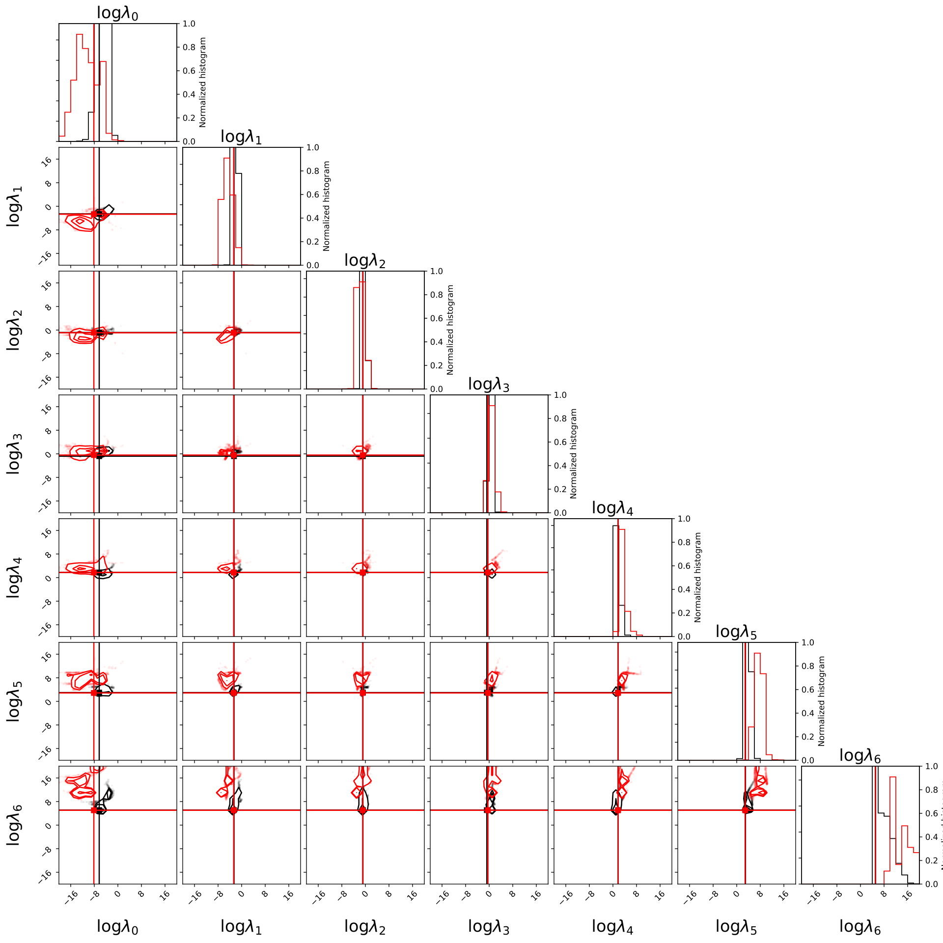
We find 1300 points to sample the DD-PC1 parameter space reasonably well. Figure 2 shows the distributions of the parameters at the beginning (denoted by black symbols and contours) and at (red symbols and contours). These two distributions are almost identical since the simulated parameters are more dispersed than the gradual changes in parameter values along the geodesic.
Even though the parameter uncertainties in the full model are large, we can estimate the error on the eigensolutions of the FIM along the geodesic. We do this by computing the FIM for every simulated point propagated along the best-fitting geodesic to various values of using the Jacobi equation. The results of this procedure are shown in Fig. 3. The top panels show the median and the corresponding confidence interval of the eigensolutions, computed using the 16th and the 84th percentile. The simulated FIM eigenvector components squared are shown in Fig. 3(a) and the FIM eigenvalues are shown in Fig. 3(b) for each . We see that, while the results using the simulated sample are consistently ordered when compared to the MBAM solution, there is a small offset between the median and the MBAM solution. Figures 3(c) and 3(d) show the median and the confidence interval for the FIM determinant and the scalar curvature, respectively. The simulated scalar curvature and the metric determinant along the geodesic show a larger variation in their values along the geodesic. In these panels we additionally show the FIM determinant and the scalar curvature along the best-fitting geodesic by the solid orange lines. There is a large discrepancy between the behavior of the median of the simulated quantities and the behavior of the quantities along the best-fitting geodesic. In Fig. 3(c) [Fig. 3(d)], we see that these quantities along the best-fitting geodesic are comparable to the 5th (95th) percentile of (scalar curvature), shown as dotted lines. This behavior indicates that only the geodesics starting at the vicinity of the best-fitting point encounter the region corresponding to .
Furthermore, in Figs. 4 and 5 we show, respectively, the distributions of eigenvalues and components of at the beginning and at the end of the geodesic. These large differences in eigenvalues and eigenvector components propagating along the geodesic are in stark contrast to the parameter values in Fig. 2. The discrepancies presented in Figs. 3, 4, and 5 can be explained by the sensitivity of the FIM eigenproblem to small changes in DD-PC1 parameters, since diagonalization results are not expected to change linearly with inputs. We conclude that the offset is due to the non-Gaussianity of the distribution of eigenvalues and components, which arises even though the parameters were sampled using the normal distribution. Even though there is a change in the shape of these distributions, the overall qualitative MBAM conclusions remain the same along the geodesic.
IV.3 Model reparametrization
The authors of Ref. (Nikšić and Vretenar 2016) have considered an exponential reparametrization of the seven-parameter DD-PC1 coupling constants centered at their best-fitting values Nikšić et al. 2008. This reparametrization transformation can be schematically represented as a vector
| (16) |
where indicates the multivariate distribution of parameters , and the quantities such as , , etc., stand for the best-fitting parameter values. The exponential form of the coupling constants is chosen by the constraints (i) that the new parameters in the geodesic equation are dimensionless and (ii) that the exponential form prevents the coupling functions and from changing sign along the geodesic path, thus confining them in the region described by the inequalities and . Using these constraints the scalar mean-field potential remains attractive and the vector mean-field remains repulsive for all allowed parameter values Nikšić and Vretenar 2016.

We repeat the Monte Carlo analysis described in Sec. IV.2 for the reparametrized model. The resulting error estimates are shown in Fig. 6 in the same manner as in Fig. 3. By comparing the two figures panel-by-panel, we conclude that both methods produce MBAM geodesics that are stable under perturbations, even though the two FIMs do not behave in the same way along their respective geodesics. The reparametrized FIM determinant and the Ricci scalar change gradually, compared to the initial model.
One may ask whether this discrepancy is due to using a too simplistic description of the reparametrized distributions. We then employ the Bayesian statistics to check whether the multivariate distribution has pronounced non-Gaussian features. To this end, we use the Markov chain Monte Carlo (MCMC) technique to sample the posterior distribution, as implemented in the package EMCEE Foreman-Mackey et al. 2013. In Fig. 7 we show the behavior of the chosen 200 Markov chains as two-dimensional sections of the parameter space. The chains have been run for a long enough time to avoid the initial “burn-in” phase characteristic of the algorithm during which they follow mostly the (uniform) prior distribution instead of sampling the posterior distribution. From the fact that the classical covariance ellipses (represented by red contours in Fig. 7) are well aligned with the MCMC estimates, we conclude that one can proceed with using the simple Monte Carlo Gaussian mock sample for error propagation instead of the computationally more expensive Bayesian MCMC mock sample.
The theoretical argument for the discrepancy between the two geodesics is based on the properties of the applied transformation. Since the exponential transformations are not bijections, the geodesics on the manifold spanned by need not have the same behavior as the geodesics on the manifold spanned by . To better understand the connection between these two geodesics, we derive the FIM determinant on the -manifold by using the transformation of Eq. (16),
| (17) |
The determinant of the metric is not an invariant quantity under reparametrizations, and hence the additional multiplicative scaling is required. Equation (17) shows that, if the value of approaches zero for particular values of , both geodesics terminate. However, additional singularities appear if any of the coupling constants are allowed to change sign along a particular geodesic. In contrast to the FIM determinant, the Ricci scalar is not affected by reparametrizations. The scalar curvature distributions for different points on the geodesic in Fig. 6(d) do not have the same values as those in Fig. 3(d). The effects of reparametrizations on the scalar curvature can be clearly seen from the comparison between these figures.
The general conclusion is, therefore, that the MBAM method is sensitive to the way the reparametrization is made, as has been shown above in the case of the reparametrization tied to domain restrictions. This is related to the fact that different reparametrizations do not lead to the same, but similar, models describing the common physical problem. Since the EDF has an arbitrarily chosen functional form, there is no a priori way of identifying which parametrization is optimal. This sensitivity only emphasizes the fact that different reparametrizations may describe similar, but inherently different, physical models. Choosing a particular EDF parametrization is equivalent to choosing a particular range model parameters can take.
V Conclusion
Methods of information geometry have been applied to investigate the stability of reducing the nuclear structure models. We have constrained the error estimates of the MBAM solutions by means of the Monte Carlo simulations. In the illustrative application to the DD-PC1 model of the nuclear EDF, it has been found that the main conclusions obtained by using the MBAM method are stable under the variation of the parameters within the confidence interval of the best-fitting model. Moreover, we have found that the end of the geodesic occurs when the determinant of the FIM approaches zero, thus effectively separating the parameter space into two disconnected regions.
Further applications of information geometry to nuclear EDFs could be analyzing possible phase transitions in models of finite nuclei using scalar curvature and their impact on nuclear properties. The analysis could even be expanded to include an extended temperature-dependent model or to look for model instabilities. It would be worth investigating whether information-theoretic optimizations could accelerate computer codes to solve nuclear many-body problems. Such second-order optimization algorithms, as the natural-gradient descent, find optimal solutions by taking optimization steps in the parameter space informed by the behavior of the FIM.
Acknowledgments
This work is financed within the Tenure Track Pilot Programme of the Croatian Science Foundation and the École Polytechnique Fédérale de Lausanne and by Project No. TTP-2018-07-3554 Exotic Nuclear Structure and Dynamics, with funds of the Croatian-Swiss Research Programme.
References
- Bender et al. (2003) M. Bender, P.-H. Heenen, and P.-G. Reinhard, Rev. Mod. Phys. 75, 121 (2003).
- Vretenar et al. (2005) D. Vretenar, A. Afanasjev, G. Lalazissis, and P. Ring, Phys. Rep. 409, 101 (2005).
- Nikolaus et al. (1992) B. A. Nikolaus, T. Hoch, and D. G. Madland, Phys. Rev. C 46, 1757 (1992).
- Bürvenich et al. (2002) T. Bürvenich, D. G. Madland, J. A. Maruhn, and P.-G. Reinhard, Phys. Rev. C 65, 044308 (2002).
- Nikšić et al. (2008) T. Nikšić, D. Vretenar, G. A. Lalazissis, and P. Ring, Phys. Rev. C 77, 034302 (2008).
- Nikšić and Vretenar (2016) T. Nikšić and D. Vretenar, Phys. Rev. C 94, 024333 (2016).
- Nikšić et al. (2017) T. Nikšić, M. Imbrišak, and D. Vretenar, Phys. Rev. C 95, 054304 (2017).
- Kortelainen et al. (2010) M. Kortelainen, T. Lesinski, J. Moré, W. Nazarewicz, J. Sarich, N. Schunck, M. V. Stoitsov, and S. Wild, Phys. Rev. C 82, 024313 (2010).
- Bogner et al. (2013) S. Bogner, A. Bulgac, J. Carlson, J. Engel, G. Fann, R. Furnstahl, S. Gandolfi, G. Hagen, M. Horoi, C. Johnson, M. Kortelainen, E. Lusk, P. Maris, H. Nam, P. Navratil, W. Nazarewicz, E. Ng, G. Nobre, E. Ormand, T. Papenbrock, J. Pei, S. Pieper, S. Quaglioni, K. Roche, J. Sarich, N. Schunck, M. Sosonkina, J. Terasaki, I. Thompson, J. Vary, and S. Wild, Comput. Phys. Commun. 184, 2235 (2013).
- Reinhard (2016) P. G. Reinhard, Phys. Scr 91, 023002 (2016).
- Dobaczewski et al. (2014) J. Dobaczewski, W. Nazarewicz, and P. G. Reinhard, J. Phys. G: Nucl. Part. Phys. 41, 074001 (2014).
- Schunck et al. (2015a) N. Schunck, J. D. McDonnell, J. Sarich, S. M. Wild, and D. Higdon, J. Phys. G: Nucl. Part. Phys. 42, 034024 (2015a).
- Schunck et al. (2015b) N. Schunck, J. D. McDonnell, D. Higdon, J. Sarich, and S. M. Wild, Eur. Phys. J. A 51, 169 (2015b).
- Piekarewicz et al. (2015) J. Piekarewicz, W.-C. Chen, and F. J. Fattoyev, J. Phys. G: Nucl. Part. Phys. 42, 034018 (2015).
- Roca-Maza et al. (2015) X. Roca-Maza, N. Paar, and G. Colò, J. Phys. G: Nucl. Part. Phys. 42, 034033 (2015).
- Agbemava et al. (2019) S. E. Agbemava, A. V. Afanasjev, and A. Taninah, Phys. Rev. C 99, 014318 (2019).
- Dedes and Dudek (2018) I. Dedes and J. Dudek, Phys. Scr 93, 044003 (2018).
- Dedes and Dudek (2019) I. Dedes and J. Dudek, Phys. Rev. C 99, 054310 (2019).
- Kejzlar et al. (2020) V. Kejzlar, L. Neufcourt, W. Nazarewicz, and P. G. Reinhard, J. Phys. G: Nucl. Part. Phys. 47, 94001 (2020).
- Taninah et al. (2020) A. Taninah, S. E. Agbemava, A. V. Afanasjev, and P. Ring, Phys. Lett. B 800, 135065 (2020).
- Amari (1982) S.-I. Amari, Ann. Stat. 10, 357 (1982).
- Amari (2016) S.-I. Amari, Information Geometry and Its Applications, Applied Mathematical Sciences (Springer Japan, Tokyo, 2016).
- Amari (1998) S.-I. Amari, Neural Comput. 10, 251 (1998).
- Ma et al. (1997) S. Ma, C. Ji, and J. Farmer, Neural Networks 10, 243 (1997).
- Transtrum et al. (2010) M. K. Transtrum, B. B. MacHta, and J. P. Sethna, Phys. Rev. Lett. 104, 060201 (2010).
- Transtrum et al. (2011) M. K. Transtrum, B. B. MacHta, and J. P. Sethna, Phys. Rev. E 83, 036701 (2011).
- Transtrum and Qiu (2014) M. K. Transtrum and P. Qiu, Phys. Rev. Lett. 113, 098701 (2014).
- Transtrum et al. (2015) M. K. Transtrum, B. B. Machta, K. S. Brown, B. C. Daniels, C. R. Myers, and J. P. Sethna, J. Chem. Phys. 143, 010901 (2015).
- Transtrum (2016) M. K. Transtrum, arXiv e-prints , arXiv:1605.08705 (2016).
- Tisanić et al. (2020) K. Tisanić, V. Smolčić, M. Imbrišak, M. Bondi, G. Zamorani, L. Ceraj, E. Vardoulaki, and J. Delhaize, Astron. Astrophys. 643, A51 (2020).
- (31) B. L. Francis and M. K. Transtrum, Unwinding the model manifold: choosing similarity measures to remove local minima in sloppy dynamical systems, Tech. Rep.
- Typel and Wolter (1999) S. Typel and H. Wolter, Nucl. Phys. A 656, 331 (1999).
- Finelli et al. (2004) P. Finelli, N. Kaiser, D. Vretenar, and W. Weise, Nucl. Phys. A 735, 449 (2004).
- Finelli et al. (2006) P. Finelli, N. Kaiser, D. Vretenar, and W. Weise, Nucl. Phys. A 770, 1 (2006).
- Baldo et al. (2008) M. Baldo, P. Schuck, and X. Viñas, Phys. Lett. B 663, 390 (2008).
- Baldo et al. (2013) M. Baldo, L. M. Robledo, P. Schuck, and X. Viñas, Phys. Rev. C 87, 064305 (2013).
- Nikšić et al. (2008) T. Nikšić, D. Vretenar, and P. Ring, Phys. Rev. C 78, 034318 (2008).
- Nikšić et al. (2011) T. Nikšić, D. Vretenar, and P. Ring, Prog. Part. Nucl. Phys. 66, 519 (2011).
- Kortelainen et al. (2012) M. Kortelainen, J. McDonnell, W. Nazarewicz, P.-G. Reinhard, J. Sarich, N. Schunck, M. V. Stoitsov, and S. M. Wild, Phys. Rev. C 85, 024304 (2012).
- Kortelainen et al. (2014) M. Kortelainen, J. McDonnell, W. Nazarewicz, E. Olsen, P.-G. Reinhard, J. Sarich, N. Schunck, S. M. Wild, D. Davesne, J. Erler, and A. Pastore, Phys. Rev. C 89, 054314 (2014).
- Bulgac et al. (2015) A. Bulgac, M. McNeil Forbes, and S. Jin, arXiv e-prints , arXiv:1506.09195 (2015), arXiv:1506.09195 [nucl-th] .
- Gutenkunst et al. (2007) R. N. Gutenkunst, J. J. Waterfall, F. P. Casey, K. S. Brown, C. R. Myers, and J. P. Sethna, PLoS Comput. Biol. 3, e189 (2007).
- Lee (2018) J. M. Lee, Introduction to Riemannian Manifolds, Graduate Texts in Mathematics (Springer International Publishing, Cham, 2018).
- Machta et al. (2013) B. B. Machta, R. Chachra, M. K. Transtrum, and J. P. Sethna, Science 342, 604 (2013).
- Agbemava et al. (2014) S. E. Agbemava, A. V. Afanasjev, D. Ray, and P. Ring, Phys. Rev. C 89, 054320 (2014).
- Agbemava et al. (2015) S. E. Agbemava, A. V. Afanasjev, T. Nakatsukasa, and P. Ring, Phys. Rev. C 92, 054310 (2015).
- Virtanen et al. (2020) P. Virtanen, R. Gommers, T. E. Oliphant, M. Haberland, T. Reddy, D. Cournapeau, E. Burovski, P. Peterson, W. Weckesser, J. Bright, S. J. van der Walt, M. Brett, J. Wilson, K. J. Millman, N. Mayorov, A. R. J. Nelson, E. Jones, R. Kern, E. Larson, C. J. Carey, I. Polat, Y. Feng, E. W. Moore, J. VanderPlas, D. Laxalde, J. Perktold, R. Cimrman, I. Henriksen, E. A. Quintero, C. R. Harris, A. M. Archibald, A. H. Ribeiro, F. Pedregosa, P. van Mulbregt, and SciPy 1.0 Contributors, Nat. Methods 17, 261 (2020).
- Foreman-Mackey et al. (2013) D. Foreman-Mackey, D. W. Hogg, D. Lang, and J. Goodman, Publ. Astron. Soc. Pac. 125, 306 (2013).