On the impact of incorporating task-information in learning-based image denoising
Abstract
A variety of deep neural network (DNN)-based image denoising methods have been proposed for use with medical images. These methods are typically trained by minimizing loss functions that quantify a distance between the denoised image, or a transformed version of it, and the defined target image (e.g., a noise-free or low-noise image). They have demonstrated high performance in terms of traditional image quality metrics such as root mean square error (RMSE), structural similarity index measure (SSIM), or peak signal-to-noise ratio (PSNR). However, it has been reported recently that such denoising methods may not always improve objective measures of image quality. In this work, a task-informed DNN-based image denoising method was established and systematically evaluated. A transfer learning approach was employed, in which the DNN is first pre-trained by use of a conventional (non-task-informed) loss function and subsequently fine-tuned by use of the hybrid loss that includes a task-component. The task-component was designed to measure the performance of a numerical observer (NO) on a signal detection task. The impact of network depth and constraining the fine-tuning to specific layers of the DNN was explored. The task-informed training method was investigated in a stylized low-dose X-ray computed tomography (CT) denoising study for which binary signal detection tasks under signal-known-statistically (SKS) with background-known-statistically (BKS) conditions were considered. The impact of changing the specified task at inference time to be different from that employed for model training, a phenomenon we refer to as “task-shift”, was also investigated. The presented results indicate that the task-informed training method can improve observer performance while providing control over the trade off between traditional and task-based measures of image quality.
Index Terms:
Objective image quality assessment, image restoration, image denoising, deep learningI Introduction
The development of image denoising methods for medical imaging applications based on deep neural networks (DNNs) remains an active area of research [1, 2, 3]. Although learning-based image denoising methods, by conventional design, can improve traditional image quality (IQ) measures such as root mean square error (RMSE) and structural similarity index measure (SSIM), it is well-known that such measures may not always correlate with objective task-based IQ measures [4, 5, 6, 7]. Here and throughout this article, a “task” denotes an image-based inference to be performed by a human or numerical observer. This is because the loss functions that are commonly employed to train such methods do not explicitly take into account the intended task that is to be performed by use of the resulting images. For example, Yu et al. [6] demonstrated that task-based metrics were not consistent with traditional IQ metrics in a study of DNN-based image denoising related to nuclear medicine imaging. Likewise, Li et al. [5] reported similar findings and systematically investigated task-related information loss induced by DNN-based denoising methods under different conditions. Task-information loss has also been studied within the context of the learning-based single-image super-resolution problem [8].
To enhance the utility of an image produced by use of a learning-based method, information regarding a task can be naturally incorporated into the training procedure [9, 10, 11, 12]. A variety of task-informed methods employ a hybrid loss comprised of a conventional and a task-based loss component. For an image reconstruction problem, Adler et al. [9] proposed such an approach to establish a learned reconstruction operator. Similarly, Ongie et al. [11] designed a low-dose CT reconstruction framework to enhance the detectability of signals. For enhancing the utility of denoised images for segmentation tasks, Zhang et al. [10] proposed a task-informed low-dose CT denoising framework that employed a hybrid loss that incorporated the dice score loss. In a different approach that did not employ the hybrid loss strategy, Han et al. [12] proposed a perceptual loss-based denoising method.
While these studies provided valuable insights into the potential of learning-based task-informed image restoration methods, this line of research is relatively new and underdeveloped. Improved utility of the restored image for the specified task generally comes at the cost of degraded task-agnostic measures of image quality, and understanding this complicated trade-off within the context of a specific problem is important. While task-related information has been incorporated into loss function designs, the use of transfer learning coupled with constraints on how such information is utilized during model fine-tuning remains unexplored. This is potentially important because previous studies have reported that task-related information may be primarily lost by the deeper layers of a DNN for certain applications [5].
Another critical issue that is specifically relevant to task-informed learning-based methods for image restoration or formation relates to generalization performance with respect to the task. Tasks in medical imaging applications are generally complicated and can be difficult to comprehensively specify, either analytically or implicitly via specification of a collection of acquired images. For example, a signal detection task requires the specification of the signal to be detected and the background in which it is embedded. Both of these quantities are generally stochastic in nature and will vary with subject and disease state in the specified cohort. When a task-informed image restoration method is trained with consideration of a specified detection task, by design, it is anticipated that the resulting images will possess enhanced utility for performing that particular task. However, at inference time, the characteristics of the signal or background may differ from those modelled in the original task. This is a phenomenon that we refer to as “task-shift”, indicating that source tasks (used for training) are different from target tasks (used for inference) [13]. Assessing the robustness of a task-informed image restoration method to task-shift is essential to understand its potential suitability for clinical translation. To date, this topic has not been explored within the context of task-informed learning-based image restoration or reconstruction methods.
To begin addressing these issues, in this work a task-informed DNN-based image denoising method is established with consideration of several signal-known-statistically (SKS) with background-known-statistically (BKS) binary signal detection tasks of varying difficulty. The method is systematically and objectively assessed by use of a stylized low-dose X-ray computed tomography (CT) denoising testbed that involves detecting lesions in denoised low-dose CT lung images. A transfer learning approach is employed, in which a DNN is pre-trained by use of a conventional (non-task-informed) loss function and subsequently fine-tuned by use of a hybrid loss that includes a task-component. The task-component is designed to measure the performance of a numerical observer (NO) on the detection task. The impact of network depth and constraining the fine-tuning to specific layers of the DNN is explored. Additionally, the impact of task-shift is investigated to assess the robustness of the approach. It is expected that the study findings will provide insights into the design and assessment of other task-informed learning-based methods for image restoration and image reconstruction.
The remainder of the paper is organized as follows. Section II describes the necessary background on DNN-based image denoising, signal detection tasks, and numerical observers. The task-informed training method is described in Section III. The numerical studies and the corresponding evaluations of the task-informed training method are provided in Sections IV and V, respectively. Finally, the article provides a discussion of the key findings in Section VI.
II Background
II-A Learning-based image denoising
End-to-end learning-based denoising methods hold significant potential for medical imaging applications [1, 14, 15, 2, 16, 17]. Given a noisy image , where is the dimension of image, an end-to-end learning-based denoising method can be described generically as:
| (1) |
where denotes an image-to-image mapping implemented by a DNN that is parameterized by the weight vector and denotes the denoised image. Depending on how the target data are defined when training the DNN, can be interpreted as an estimate of the noiseless image or an estimate of a reduced noise version of . A variety of DNNs have been employed to implement the mapping [2, 17, 18], and convolutional neural networks (CNNs) represent a popular choice [19, 15, 20, 1, 2, 3].
In addition to the choice of DNN architecture, the specification of the loss function plays a key role in the design of a DNN-based denoising method. Mean square error (MSE) that measures the distance between the denoised and target images has been widely employed [1, 14, 19, 15, 20, 16, 21, 17]. The perceptual loss function has also been used and was reported to be effective in reducing noise while retaining image details [2], and use of adversarial loss functions have been deployed with similar success [22, 14]. However, such loss functions that are commonly employed in computer vision applications do not explicitly incorporate information regarding a particular medical imaging task. In recent studies, it has been demonstrated that learning-based denoising methods trained by use of such loss functions can improve traditional IQ measures such as RMSE or SSIM while important information relevant to a downstream detection task is lost [5, 6]. Such findings motivate the further development and investigation of task-informed learning-based denoising methods.
II-B Formulation of binary signal detection task
In this study, a binary signal detection task is considered that requires an observer to classify a denoised image as satisfying either a signal-present hypothesis or a signal-absent hypothesis . These two hypotheses can be described as:
| (2a) | |||
| (2b) |
where and denote signal-present and signal-absent noiseless images and denotes the measurement noise. A signal-present image is formulated by inserting a signal image into a background object . In a SKE detection task, is non-random, whereas in a SKS detection task it is a random process. Similarly, in a BKE detection task, is nonrandom, whereas in a BKS detection task it is a random process. To perform this task, a deterministic observer computes a test statistic that maps the image to a real-valued scalar test statistic, which is used to perform the task.
II-C Numerical observers for objective IQ assessment
In preliminary assessments of medical imaging technologies, numerical observers (NOs) have been employed to quantify task-based measures of IQ for various image-based inferences[23]. The NOs that are employed in this study are surveyed below.
II-C1 Hotelling Observer
The Hotelling Observer (HO) employs the Hotelling discriminant, which is the population equivalent of the Fisher linear discriminant, and is optimal among all linear observers in the sense that it maximizes the signal-to-noise ratio of the test statistic [4, 24]. The HO test statistic computed by use of the denoised data is defined as:
| (3) |
where denotes the Hotelling template, denotes the difference between the ensemble mean of the image data under the two hypotheses and , and . Here, and denote the covariance matrices corresponding to under and , respectively.
In some cases, the covariance matrices and are ill-conditioned and therefore their inverse cannot be stably computed. To address this, a regularized HO (RHO) can be employed that implements the test statistic as [5]:
| (4) |
where represents a low-rank approximation of that is formed by keeping only the singular values of greater than . Here, is a tunable parameter and represents the largest singular value of . Finally, is the Moore–Penrose inverse of .
It has been demonstrated that when data with large dimensions are considered, the estimation and inversion of the covariance matrix can be intractable [25], which makes the implementation of the HO challenging. To circumvent this difficulty, a supervised learning-based method that uses a simple single layer neural network (SLNN) to approximate the HO has been proposed recently [26]. The HO discriminant function can be modeled by a SLNN that possesses only a single fully-connected layer. This SLNN-approximated HO (SLNN-HO) directly learns the Hotelling template without explicitly estimating and inverting covariance matrices. It has been reported that the SLNN-HO is effective with large images and a limited number of images [26].
II-C2 Channelized Hotelling observer
A channelized HO (CHO) is formed when the HO is employed with a channeling mechanism. When implemented with anthropomorphic channels and an internal noise mechanism, the CHO can be interpreted as an anthropomorphic observer and attempts to predict human observer performance [27, 28]. In addition, the channeling mechanism can also be employed to reduce the dimensionality of the image data when the image data is insufficient to accurately estimate the covariance matrix. Let denote a channel matrix and the corresponding channelized image data. The CHO test statistic is given by:
| (5) |
where denotes the covariance matrix of the channelized data , denotes the covariance matrix of the channel internal noise, and is a noise vector sampled from a Gaussian distribution . Based on previous studies [28], in this work is defined as:
| (6) |
where represents a diagonal matrix with diagonal elements from and is the internal noise level. The parameters of the difference-of-Gaussian (DOG) channels and the internal noise level employed in this study are described below in Section IV-C4.
II-C3 Learned NOs
Recently, several machine learning methods have been proposed to establish NOs [26, 29, 30]. The SLNN-based NO (SLNN-NO) is a special learned NO that has the shallowest architecture that possesses only a single fully-connected layer with a bias term and a sigmoid activation function. The binary cross entropy (BCE) loss function can be used to train the SLNN-NO.
III Task-informed training method
In this work, a transfer learning approach is investigated in which a DNN is pre-trained by use of a conventional (non-task-informed) loss function and subsequently fine-tuned by use of a hybrid loss that includes a task-component . The fine-tuning of the denoising network is constrained to the last several layers instead of re-training the whole network. This is motivated by a recent study by Li et al.[5] that demonstrated, at least for linear CNN-based denoising networks, the degradation of task-relevant information primarily occurs in the last layers. A hybrid loss function is defined as [9]:
| (7) |
where is a scalar parameter, is the physical loss component, is the task-component, is the vector of weight parameters associated with the trainable layers in the pretrained denoising network, and denotes the vector of weight parameters of the NN-based NO used to compute the task-component . The task-component is designed to measure the performance of a NO on a specific task. By appending a network-based NO to the pretrained denoising network, the denoised image can be transformed into a scalar that is used to compute the task-specific component. The trainable layers in the pretrained denoising network are jointly trained with the NO. By employing this training strategy, the NO used to compute can be easily adapted to different tasks. The details of the proposed task-informed training method are described below and summarized in Algorithm 1.
Mean-squared-error (MSE) and mean-absolute-error (MAE) are commonly employed choices for . The selection of the task-based loss component is based on specific tasks. In this paper, binary signal detection tasks were considered, and the specific formulation of is described in Section IV-B.
- •
: Weight parameters of the denoising network with layers;
- •
: Weight parameters of the last trainable layers of ;
- •
: Weight parameters of the first layers of the denoising network , };
- •
: Weight parameters of an appended observer used to compute the task-component ;
- •
: Physical loss for pre-training and task-informed training ;
- •
: Task-based loss for task-informed training ;
- •
: The hybrid loss formulated by and , and weighted by the parameter defined in Eqn. (7);
- •
: Dataset for pre-training ;
- •
: Dataset for task-informed training ;
- 1.
Given initial setting of parameters , pretrain the denoising network and optimize weight parameters by use of and physical loss function ;
- 2.
Append the observer with weight parameters to the pretrained ;
- 3.
Set the weight parameters that correspond to the last convolutional layers of the pretrained to be trainable;
// The other trained weight parameters are fixed; - 4.
Given initial setting of and pre-trained , jointly tune the weight parameters and train by use of and the hybrid loss function ;
- 5.
Output the task-informed denoising network with optimized weight parameters .
IV Numerical studies
In this paper, the task-informed training method in Algorithm 1 was objectively assessed in a stylized low-dose X-ray computed tomography (CT) denoising study. Binary signal detection tasks under signal-known-statistically (SKS) with background-known-statistically (BKS) conditions were considered. Both the SLNN-NO and SLNN-HO were considered as the NOs employed to compute the task-component in Eqn. (7). The performance of the SLNN-NO, SLNN-HO, and other NOs described in Sec. II-C on denoised images was quantified to evaluate the impact of task-informed training procedure on the denoising network. The details of numerical studies are described below.
IV-A Virtual imaging pipeline
The Lung Image Database Consortium image collection (LIDC) [31] was employed to generate signal-present (SP) images and signal-absent (SA) images to perform binary signal detection tasks as defined in Eqn. (2). This database consists of 243,945 2D image slices from 1,018 3D thoracic CT reconstructed images, in which 10,706 image slices contain annotated nodules. In addition to the 10,706 SP images, additional SP images were generated by inserting realistic nodules using an established insertion method [32]. Fifty-thousand SA images were formed by extracting regions-of-interest (ROIs) of dimension of pixels from normal lung areas from central several slices. The same number of SP images were generated. In SP images, the centroids of the nodules were either located at a fixed location or at random locations subject to the specific tasks described in Section IV-C. The generated SP and SA images were utilized as the target (normal-dose) CT images .
The corresponding noise-enhanced (low-dose) images were generated by degrading the target images described above. The target image was first transformed to the projection domain by using the 2D discrete Radon transform . Noise-enhanced projection were generated by adding Poisson noise to the transmission data, which is described as:
| (8) |
Here, was a Poisson random vector, , and , where is a scalar used for normalization and the parameter controlled noise level [33]. The noisy (low-dose) images were then reconstructed by use of a filtered back-projection (FBP) reconstruction algorithm that employed a Ram-Lak filter [34]. Samples of the generated images are shown in Fig. 1. The pairs of noisy and target images are used for training the denoising method described below in Section IV-B.

IV-B Training and validation details
IV-B1 Architecture and loss function for denoising networks
The canonical CNN architecture of depth depicted in Fig. 2 was employed with the task-informed training method to establish an end-to-end learned denoising method. It is important to note that the assessment studies described below can be readily repeated with any other DNN. The network input was a reconstructed noisy image of dimension and the output was a denoised image with the same dimensions. The CNN contained four types of layers. The first layer was a Conv+ReLU layer, in which 64 convolution filters of dimension were applied to generate 64 feature maps. In each of the to Conv+BN+ReLU layers, 64 convolution filters of dimension were employed and batch normalization was included between the convolution and ReLU operations. In the Conv+BN layer, 64 convolution filters of dimension were employed and batch normalization was performed. In the last Conv layer, one single convolution filter of dimension was employed to form the final denoised image of dimension .
Let denote a given SA or SP target (normal-dose) image and let denote the corresponding noise-enhanced (low-dose) image. Given a collection of paired training data , the denoising network was pretrained by minimizing the MSE loss function:
| (9) |
where the vector denotes the weight parameters of the denoising network.

IV-B2 Architecture and loss function for the NN-based observers used to compute
The physical loss function in Eqn. (7) was defined by a MSE loss. The task-component of the hybrid loss function was computed by use of either the SLNN-NO or SLNN-HO as described next.
The SLNN-NO consisted of a fully-connected layer along with a sigmoid activation function. The BCE loss function was employed to train the SLNN-NO. Let denote the image data and the corresponding label . The BCE loss function can be expressed as [26]:
| (10) |
Here, is the vector of weight parameters associated with the trainable layers in the pretrained denoising network, and the vector denotes the weight parameters of the fully-connected layer of the appended SLNN-NO.
IV-B3 Datasets and denoising network training details
The standard convention of utilizing separate training/validation/testing datasets was adopted. The training dataset included 40,000 pairs of noisy signal-present and signal-absent images along with the corresponding target (normal noise) images. The validation dataset including 200 signal-present images and 200 signal-absent images and the corresponding target (normal noise) images was randomly selected from the training dataset. Finally, the testing dataset comprised 10,000 signal-present images and 10,000 signal-absent noisy images. For task-informed model training with the hybrid loss function , the same training dataset described above was employed to fine-tune the denoising network. The validation and testing datasets used for pretraining were also employed to evaluate the performance of the fine-tuned denoising networks.
In both the pretraining and task-informed fine-tuning stages, the denoising networks were trained on mini-batches at each iteration by use of the Adam optimizer [35] with a learning rate of 0.0001. Each mini-batch contained 50 signal-present images and 50 signal-absent images that were randomly selected from the training dataset. The network model that possessed the best performance on the validation dataset was selected for use. The Keras library [36] was employed for implementing and training all networks on a single NVIDIA TITAN X GPU.
IV-C Objective evaluation of image quality
IV-C1 SKS/BKS binary signal detection tasks with fixed signal locations
The task-informed training method was evaluated for SKS/BKS binary signal detection tasks where known signal locations were considered. The centroids of the nodules were located at the center of the extracted ROIs. The incident flux was used to determine the noise level in simulated noisy images.
Both the SLNN-NO and SLNN-HO were employed as NOs used to compute task component in Eqn. (7). The SLNN-NO, HO, RHO, and DOG-CHO were employed for subsequent assessments of image quality. It should be noted that for the case where the SLNN-NO was employed to compute , the SLNN-NO employed for objective image quality assessment was trained on the denoised estimates and it was not identical to that used to compute . The weight parameters in Eqn. (7) were considered. Only the last three convolutional layers of the denoising network were set to be trainable for both cases. Based on these settings, the impact of the weight parameter on the performance of considered NOs was investigated.
IV-C2 SKS/BKS binary signal detection tasks with random signal locations
In this case, the centroids of the nodules were randomly located within the lung area of extracted ROIs by use of a uniform probability density function. The incident flux was used to determine the noise level of the simulated low-dose images. The SLNN-NO was used to compute task component in Eqn. (7), considering that the SLNN-NO can be employed when signal is randomly located. The trained SLNN-NO was subsequently utilized to evaluate the performance of fine-tuned denoising networks. This represented a situation that the same observer was used for both training and evaluation.
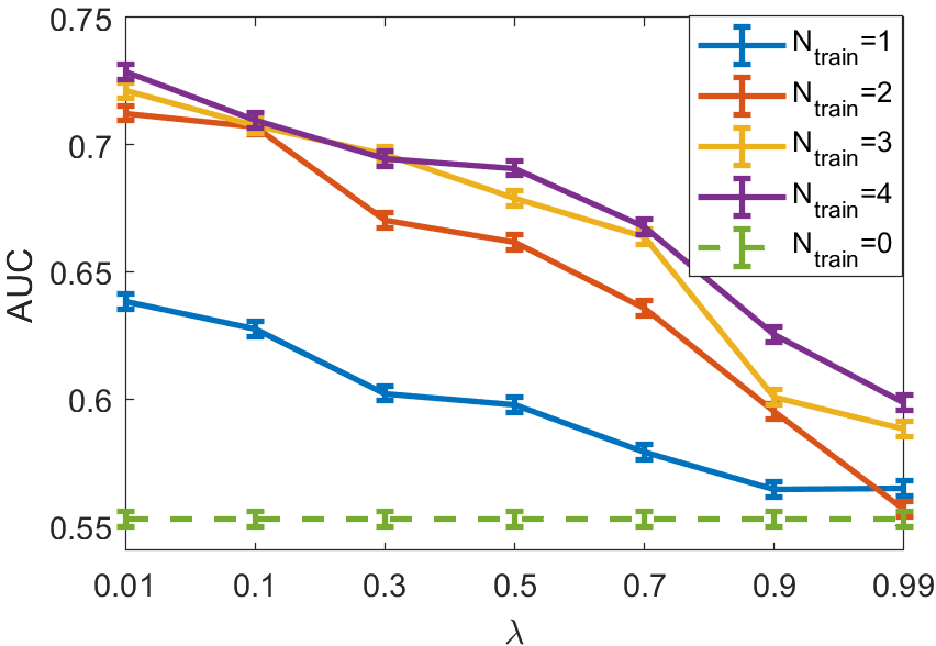
To assess the impact of the weight parameter on the performance of the SLNN-NO, the weight parameters in Eqn. (7) were considered. The number of trainable layers was also swept from 0 to 4.
IV-C3 Investigation of the task shifts in considered binary signal detection tasks
A study was designed to investigate the robustness of the task-informed image denoising method to task-shift. First, binary signal detection tasks with fixed signal locations were considered for model training (source tasks) while tasks with random signal locations were considered for evaluation (target tasks). Next, the tasks with random signal locations were used as source tasks and the tasks with fixed locations were considered as target tasks. The SLNN-NO was employed to compute task component in Eqn. (7) and only the last three convolutional layers were set to be trainable. For evaluations, SLNN-NOs were independently trained on training datasets for target tasks. The SLNN-NO performance under the situations without task shift was considered as the reference. The weight parameters in Eqn. (7) were considered to investigate the impact of task shifts when the weight of task-based component varies.
IV-C4 Numerical observer computation
Both the HO and RHO were employed for objective image quality assessment since they are optimal linear observers. For computing the HO and RHO test statistics, the covariance matrix was empirically estimated by use of 40,000 signal-present and 40,000 signal-absent images. When computing the RHO test statistic, the threshold parameter in Eqn. (4) was swept from to and the corresponding detection performance was estimated based on a separate validation dataset including 200 signal-present images and 200 signal-absent images. The value which led to the best RHO detection performance was selected.
For computing the CHO test statistic, 2,000 signal-present and 2,000 signal-absent images were utilized to empirically estimate the channelized covariance matrix. A set of 10 DOG channels [28] was employed with channel parameters , , and . The internal noise level was 2.5, which was the same value employed by Abbey et al.[28].
To independently train the SLNN-NO for objective image quality assessment, 40,000 signal-present images and 40,000 signal-absent images were employed. These learned-NOs were trained by use of the Adam optimizer [35] with a learning rate of 0.0001.
IV-C5 Evaluation metrics
Both traditional and task-based measures of IQ were employed for assessments. Receiver operating characteristic (ROC) analysis was conducted and area under the curve (AUC) values were computed and employed as a figure-of-merit for task-based measures. The ROC curves were fit by use of the Metz-ROC software [37] that employs the proper binormal model [38]. The uncertainty of the AUC values were estimated as well. Two commonly used traditional metrics (i.e., RMSE and SSIM) were employed as task-agnostic measures to assess the denoised images.
V Results
V-A Results for the case with fixed signal locations
V-A1 Impact of the weight parameter
The impact of the weight parameter in Eqn. (7) on signal detection performance as measured by AUC is shown in Fig. 3. Both the SLNN-NO and SLNN-HO described in Sec. IV-B2 were considered as the NO to compute task component in Eqn. (7). Signal detection performance was evaluated by use of the SLNN-NO, HO, RHO, and DOG-CHO acting on the denoised images. For both cases, the performance of the four different NOs on the denoised images was higher when smaller values (larger weight for task-based loss) were considered. Those results confirm that the task-informed training method can improve the NOs performance even when the NOs employed for objective image quality assessment were different from the NO used to compute during model training.
Figure 3 yields two additional noteworthy findings. First, for the case where the SLNN-HO was employed for training (top figure), the performance of the HO employed for objective image quality assessment was relatively high (statistically equivalent to that of the SLNN-NO and RHO). However, this relatively high HO performance was only observed for very small values (e.g., 0.01) in the case where SLNN-NO (bottom figure) was employed. The HO performance was much lower when relatively large values (i.e., 0.1-0.99) were employed. The RHO performance was employed as a reference and was relatively high for all cases. These observations suggest that for the case where SLNN-HO was employed for training, the second- and potentially higher-order statistical properties of the images were optimized to benefit the HO performance while such behavior did not occur in the case where SLNN-NO was considered with large values. Second, when SLNN-HO was used for training, the performance of DOG-CHO was greatly improved for small values and was not significantly improved for other cases. This observation indicates that the DOG channels were ”closer” to efficient channels when was appropriately selected. However, this behavior was not observed in the case where SLNN-NO was employed for training.


V-A2 Changes in covariance matrix induced by task-informed training method
To gain insights into the behavior of HO performance, the singular value spectra of the covariance matrices corresponding to the images denoised by task-informed training method were further examined. The results, shown in Fig. 4, reveal that the covariance matrix corresponding to the denoised images produced by use of the pretrained denoising network was ill-conditioned, while that corresponding to the denoised images produced by use of the fine-tuned denoising network was well-conditioned when SLNN-HO was employed to compute the task-component in Eqn. (7). However, for the case where SLNN-NO was employed to compute , a similar observation only occurred for very small values (e.g., 0.01) in Eqn. (7), and the covariance matrices were still ill-conditioned for large values (bottom figure). The results of this analysis were consistent with the previously discussed results shown in Fig. 3, and indicated that the task-informed training method may improve the image statistics that are important for signal detection.


V-B Results for the case with random signal locations
V-B1 Impact of the weight parameter and number of trainable layers
The impacts of the weight parameter in Eqn. (7) and the number of trainable layers on signal detection performance as measured by the SLNN-NO are shown in Figs. 5 and 6, respectively. Here the SLNN-NO employed to compute the task-component in Eqn. (7) was also employed to assess signal detection performance. For comparison, the impact on traditional measures of IQ is demonstrated in Table I. It was observed that, after the task-informed model training, the SLNN-NO signal detection performance was improved while the traditional measures of IQ were degraded compared with those achieved by the pre-trained denoising network.
As shown in Fig. 5 and Table I, for all numbers of trainable layers, the task performance increased while decreased. In addition, the degradation of traditional metrics was significant for relatively small while insignificant for large values (i.e., ). As expected, the trade off between traditional and task-based measures of IQ can be controlled by . For example, when , the resulted AUC value was greatly improved to that of , while the RMSE and SSIM were statistically equivalent to that of .
As shown in Fig. 6, for relatively small (i.e. where the task-based component is highly weighted), significant improvements in task performance were achieved by fine-tuning the last (or last several) convolutional layer(s) (e.g., 0-2) while improvement was insignificant when more layers were trainable. In addition, when larger values (i.e., ) were selected, the improvement in task performance was irrelevant to the number of trainable layers. For traditional IQ metrics (i.e., RMSE, SSIM), Table I showed that the degradation mainly resulted from the last small number of convolutional layer(s). For larger values (i.e., ), the changes in traditional IQ metrics were statistically insignificant.
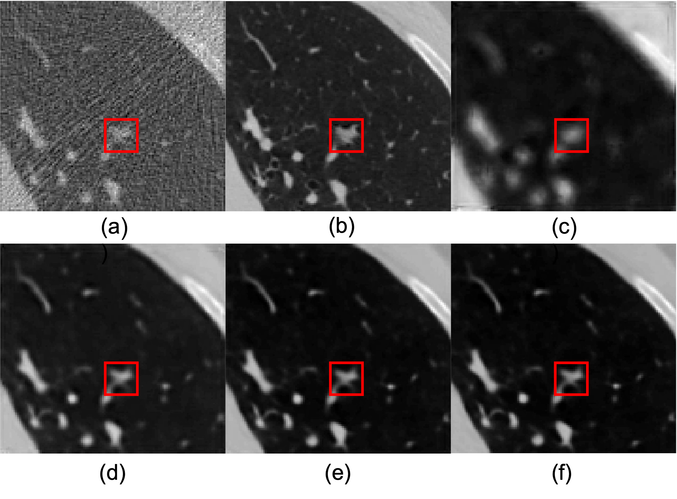
The denoised estimates produced by the task-informed image denoising methods were also subjectively assessed. Figure 7 shows a noisy image and denoised images generated by denoising networks fine-tuned with the hybrid loss for different values of in Eqn. (7). The denoised estimates were blurred as a result of the task-informed training, and the level of blur increased when decreased.

| 0 | 1 | 2 | 3 | 4 | ||
|---|---|---|---|---|---|---|
| RMSE | 0.01 | 1.3437 | 1.7178 | 1.9304 | 2.1127 | 2.2595 |
| 0.1 | 1.3437 | 1.3775 | 1.3988 | 1.4147 | 1.4244 | |
| 0.3 | 1.3437 | 1.3509 | 1.3549 | 1.3613 | 1.3667 | |
| 0.5 | 1.3437 | 1.3506 | 1.3514 | 1.3534 | 1.3546 | |
| 0.7 | 1.3437 | 1.3507 | 1.3506 | 1.3501 | 1.3498 | |
| 0.9 | 1.3437 | 1.3503 | 1.3499 | 1.3498 | 1.3495 | |
| 0.99 | 1.3437 | 1.3498 | 1.3485 | 1.3481 | 1.3477 | |
| SSIM | 0.01 | 0.9416 | 0.9197 | 0.9024 | 0.8755 | 0.8738 |
| 0.1 | 0.9416 | 0.9391 | 0.9381 | 0.9369 | 0.9368 | |
| 0.3 | 0.9416 | 0.9404 | 0.9401 | 0.9394 | 0.9391 | |
| 0.5 | 0.9416 | 0.9405 | 0.9407 | 0.9407 | 0.9408 | |
| 0.7 | 0.9416 | 0.9407 | 0.9408 | 0.9409 | 0.9409 | |
| 0.9 | 0.9416 | 0.9407 | 0.9409 | 0.9411 | 0.9412 | |
| 0.99 | 0.9416 | 0.9408 | 0.9409 | 0.9410 | 0.9414 |
V-B2 Impact of denoising network depth
A study was performed to investigate whether the loss of task-relevant information primarily occurs in the last several layers when the denoising network depths increase. As shown in Table II, the SLNN-NO performance decreased as a function of denoising network depth, which is consistent with previous findings [5] that the mantra ”deep is better” may not always hold true for objective IQ measures. After the task-informed training, the SLNN-NO performance was improved and the variations of the improved SLNN-NO performance were statistically insignificant when network depth varied. No matter how deep the pretrained denoising network was, the loss of task-relevant information still occurred in the last certain layers (i.e., not related to the depth of denoising networks), at least in the considered cases.
| 9 | 11 | 13 | 15 | |
|---|---|---|---|---|
| AUC (Fine-tuned) | 0.6984 | 0.7146 | 0.7074 | 0.7130 |
| AUC (Pretrained) | 0.5751 | 0.5714 | 0.5529 | 0.5501 |
V-C Impact of the task shifts for training and evaluation


The robustness of the task-informed image denoising method to task-shift was also assessed and the results are shown in Fig. 8. The SLNN-NO performance for the case with no task shift was considered as a reference. It was observed that introducing task shift always degraded the task performance as expected and the degradation resulting from task shift became insignificant when increased. This is due to the smaller weight for the task-based loss component as increases, which makes the impact of task shift less significant. For the case where a relatively simple task was used for training and the complex one was used for evaluation (top figure in Fig. 8), the degradation in task performance was much more significant than in the case where a complex task was used for training and a simple one was used for evaluation (bottom figure in Fig. 8). This observation is due to the fact that the case with random signal locations can be easily generalized to the case with fixed signal locations but not vice versa. This suggested that employing a relatively complex task for training can better improve the robustness of a task-informed image restoration method to task-shift than employing a simple task.
VI Discussion and Summary
In this work, a task-informed DNN-based image denoising method that preserves task-specific information was objectively evaluated. This study was motivated by previous works [5, 6] that indicate traditional DNN-based denoising methods may not benefit task performance even though the traditional measures of IQ were improved. The task-informed model training method employed a hybrid loss strategy and only acted on the last several layers of a DNN-based denoising method. To evaluate the method, binary signal detection tasks with fixed and random signal locations under SKS/BKS conditions were considered. The performance of SLNN-NO, SLNN-HO, and common NOs was quantified to assess the impact of task-informed training on task performance preservation.
The numerical results indicated that, in the cases considered, the task-informed training method could preserve task-relevant information in the image and control the trade off between traditional and task-based measures of IQ. The performance of the task-informed training method was influenced by the weight parameter , the number of trainable layers, the depth of denoising network, and the task complexity. The evaluation also confirmed that traditional IQ metrics may not always correlate with task-based metrics. Additional insights were gained by performing singular value spectra analysis. It was revealed that the method could mitigate the ill-conditioning of covariance matrices and have the potential to improve the image statistics that are important for signal detection.
To better understand the potential suitability of a task-informed image restoration method for clinical translation, its robustness to task-shift was also assessed. It was observed that introducing task-shift will degrade the task performance as expected. The degradation was significant when a relatively simple task was considered as source task while a complex one was used as target task. The degradation can be potentially mitigated by employing the complex task as source task and the simple one as target task. This suggests that employing a relatively complex task for training can better improve the robustness of a task-informed image restoration method to task-shift than employing a simple task.
There remain numerous important topics for future investigation. In this work, the SLNN-NO and SLNN-HO were employed to compute the task-component in Eqn. (7). Anthropomorphic numerical observers (ANOs) may instead be employed to predict human observer performance [28, 39, 40]. Employing an ANO to compute may potentially benefit a task-informed image denoising method if humans are the ultimate readers of the image. The evaluation study in this paper focuses on significant parameters such as the weight parameter in Eqn. (7) and the number of trainable layers. Other parameters, such as the size of training dataset and the ratio between signal-present and signal-absent images, remain unexplored. The extension of the proposed method for use with more complex tasks such as detection-estimation tasks [30, 41] is also an important topic. The task-informed image denoising method and the corresponding assessment strategy can also readily be applied to different image restoration and reconstruction methods. Ultimately, it will be critical to conduct human reader studies to assess the benefit of any task-informed method.
References
- [1] K. Zhang, W. Zuo, Y. Chen, D. Meng, and L. Zhang, “Beyond a Gaussian denoiser: Residual learning of deep CNN for image denoising,” IEEE Transactions on Image Processing, vol. 26, no. 7, pp. 3142–3155, 2017.
- [2] K. Gong, J. Guan, C.-C. Liu, and J. Qi, “PET image denoising using a deep neural network through fine tuning,” IEEE Transactions on Radiation and Plasma Medical Sciences, vol. 3, no. 2, pp. 153–161, 2018.
- [3] X. You, N. Cao, H. Lu, M. Mao, and W. Wanga, “Denoising of MR images with Rician noise using a wider neural network and noise range division,” Magnetic Resonance Imaging, vol. 64, pp. 154–159, 2019.
- [4] H. H. Barrett and K. J. Myers, Foundations of image science. John Wiley & Sons, 2013.
- [5] K. Li, W. Zhou, H. Li, and M. A. Anastasio, “Assessing the impact of deep neural network-based image denoising on binary signal detection tasks,” IEEE Transactions on Medical Imaging, 2021.
- [6] Z. Yu, M. A. Rahman, T. Schindler, R. Gropler, R. Laforest, R. Wahl, and A. Jha, “AI-based methods for nuclear-medicine imaging: Need for objective task-specific evaluation,” Journal of Nuclear Medicine, vol. 61, no. supplement 1, pp. 575–575, 2020.
- [7] K. Li, W. Zhou, H. Li, and M. A. Anastasio, “Task-based performance evaluation of deep neural network-based image denoising,” in Medical Imaging 2021: Image Perception, Observer Performance, and Technology Assessment, vol. 11599. International Society for Optics and Photonics, 2021, p. 115990L.
- [8] X. Zhang, V. A. Kelkar, J. Granstedt, H. Li, and M. A. Anastasio, “Impact of deep learning-based image super-resolution on binary signal detection,” Journal of Medical Imaging, vol. 8, no. 6, p. 065501, 2021.
- [9] J. Adler, S. Lunz, O. Verdier, C.-B. Schönlieb, and O. Öktem, “Task adapted reconstruction for inverse problems,” Inverse Problems, 2021.
- [10] J. Zhang, H. Chao, X. Xu, C. Niu, G. Wang, and P. Yan, “Task-oriented low-dose CT image denoising,” in International Conference on Medical Image Computing and Computer-Assisted Intervention. Springer, 2021, pp. 441–450.
- [11] G. Ongie, E. Y. Sidky, I. S. Reiser, and X. Pan, “Optimizing model observer performance in learning-based CT reconstruction,” in Medical Imaging 2022: Image Perception, Observer Performance, and Technology Assessment, vol. 12035. SPIE, 2022, pp. 55–59.
- [12] M. Han, H. Shim, and J. Baek, “Low-dose CT denoising via convolutional neural network with an observer loss function,” Medical Physics, vol. 48, no. 10, pp. 5727–5742, 2021.
- [13] S. J. Pan and Q. Yang, “A survey on transfer learning,” IEEE Transactions on Knowledge and Data Engineering, vol. 22, no. 10, pp. 1345–1359, 2009.
- [14] Q. Yang, P. Yan, Y. Zhang, H. Yu, Y. Shi, X. Mou, M. K. Kalra, Y. Zhang, L. Sun, and G. Wang, “Low-dose CT image denoising using a generative adversarial network with wasserstein distance and perceptual loss,” IEEE Transactions on Medical Imaging, vol. 37, no. 6, pp. 1348–1357, 2018.
- [15] Z. Li, L. Yu, J. D. Trzasko, D. S. Lake, D. J. Blezek, J. G. Fletcher, C. H. McCollough, and A. Manduca, “Adaptive nonlocal means filtering based on local noise level for CT denoising,” Medical Physics, vol. 41, no. 1, p. 011908, 2014.
- [16] H. Chen, Y. Zhang, W. Zhang, P. Liao, K. Li, J. Zhou, and G. Wang, “Low-dose CT denoising with convolutional neural network,” in 2017 IEEE 14th International Symposium on Biomedical Imaging (ISBI 2017). IEEE, 2017, pp. 143–146.
- [17] W. Jifara, F. Jiang, S. Rho, M. Cheng, and S. Liu, “Medical image denoising using convolutional neural network: a residual learning approach,” The Journal of Supercomputing, vol. 75, no. 2, pp. 704–718, 2019.
- [18] K. He, X. Zhang, S. Ren, and J. Sun, “Deep residual learning for image recognition,” in Proceedings of the IEEE Conference on Computer Vision and Pattern Recognition, 2016, pp. 770–778.
- [19] A. Manduca, L. Yu, J. D. Trzasko, N. Khaylova, J. M. Kofler, C. M. McCollough, and J. G. Fletcher, “Projection space denoising with bilateral filtering and CT noise modeling for dose reduction in CT,” Medical Physics, vol. 36, no. 11, pp. 4911–4919, 2009.
- [20] A. Le Pogam, H. Hanzouli, M. Hatt, C. C. Le Rest, and D. Visvikis, “Denoising of PET images by combining wavelets and curvelets for improved preservation of resolution and quantitation,” Medical Image Analysis, vol. 17, no. 8, pp. 877–891, 2013.
- [21] J. V. Manjón, P. Coupé, A. Buades, D. L. Collins, and M. Robles, “New methods for MRI denoising based on sparseness and self-similarity,” Medical Image Analysis, vol. 16, no. 1, pp. 18–27, 2012.
- [22] J. M. Wolterink, T. Leiner, M. A. Viergever, and I. Išgum, “Generative adversarial networks for noise reduction in low-dose CT,” IEEE Transactions on Medical Imaging, vol. 36, no. 12, pp. 2536–2545, 2017.
- [23] H. H. Barrett, J. Yao, J. P. Rolland, and K. J. Myers, “Model observers for assessment of image quality,” Proceedings of the National Academy of Sciences, vol. 90, no. 21, pp. 9758–9765, 1993.
- [24] R. A. Fisher, “The use of multiple measurements in taxonomic problems,” Annals of Eugenics, vol. 7, no. 2, pp. 179–188, 1936.
- [25] H. H. Barrett, K. J. Myers, B. D. Gallas, E. Clarkson, and H. Zhang, “Megalopinakophobia: its symptoms and cures,” in Medical Imaging 2001: Physics of Medical Imaging, vol. 4320. SPIE, 2001, pp. 299–307.
- [26] W. Zhou, H. Li, and M. A. Anastasio, “Approximating the ideal observer and Hotelling observer for binary signal detection tasks by use of supervised learning methods,” IEEE Transactions on Medical Imaging, vol. 38, no. 10, pp. 2456–2468, 2019.
- [27] K. J. Myers and H. H. Barrett, “Addition of a channel mechanism to the ideal-observer model,” Journal of the Optical Society of America A, vol. 4, no. 12, pp. 2447–2457, 1987.
- [28] C. K. Abbey and H. H. Barrett, “Human-and model-observer performance in ramp-spectrum noise: effects of regularization and object variability,” Journal of the Optical Society of America A, vol. 18, no. 3, pp. 473–488, 2001.
- [29] W. Zhou, H. Li, and M. A. Anastasio, “Approximating the ideal observer for joint signal detection and localization tasks by use of supervised learning methods,” IEEE Transactions on Medical Imaging, pp. 1–1, 2020.
- [30] K. Li, W. Zhou, H. Li, and M. A. Anastasio, “A hybrid approach for approximating the ideal observer for joint signal detection and estimation tasks by use of supervised learning and markov-chain monte carlo methods,” IEEE Transactions on Medical Imaging, 2021.
- [31] S. G. Armato III, G. McLennan, L. Bidaut, M. F. McNitt-Gray, C. R. Meyer, A. P. Reeves, B. Zhao, D. R. Aberle, C. I. Henschke, E. A. Hoffman et al., “The lung image database consortium (LIDC) and image database resource initiative (IDRI): a completed reference database of lung nodules on CT scans,” Medical Physics, vol. 38, no. 2, pp. 915–931, 2011.
- [32] A. Pezeshk, B. Sahiner, R. Zeng, A. Wunderlich, W. Chen, and N. Petrick, “Seamless insertion of real pulmonary nodules in chest CT exams,” in Medical Imaging 2014: Computer-Aided Diagnosis, vol. 9035. International Society for Optics and Photonics, 2014, p. 90351K.
- [33] D. Zeng, J. Huang, Z. Bian, S. Niu, H. Zhang, Q. Feng, Z. Liang, and J. Ma, “A simple low-dose x-ray CT simulation from high-dose scan,” IEEE Transactions on Nuclear Science, vol. 62, no. 5, pp. 2226–2233, 2015.
- [34] A. C. Kak and M. Slaney, Principles of computerized tomographic imaging. SIAM, 2001.
- [35] D. P. Kingma and J. Ba, “Adam: A method for stochastic optimization,” arXiv preprint arXiv:1412.6980, 2014.
- [36] F. Chollet et al., “Keras,” https://keras.io, 2015.
- [37] C. Metz, “ROC-kit user’s guide,” Chicago, Department of Radiology, University of Chicago, 1998.
- [38] L. L. Pesce and C. E. Metz, “Reliable and computationally efficient maximum-likelihood estimation of “proper” binormal ROC curves,” Academic Radiology, vol. 14, no. 7, pp. 814–829, 2007.
- [39] Y. Zhang, B. T. Pham, and M. P. Eckstein, “The effect of nonlinear human visual system components on performance of a channelized Hotelling observer in structured backgrounds,” IEEE Transactions on Medical Imaging, vol. 25, no. 10, pp. 1348–1362, 2006.
- [40] M. Han and J. Baek, “A convolutional neural network-based anthropomorphic model observer for signal-known-statistically and background-known-statistically detection tasks,” Physics in Medicine & Biology, vol. 65, no. 22, p. 225025, 2020.
- [41] E. Clarkson, “Estimation receiver operating characteristic curve and ideal observers for combined detection/estimation tasks,” Journal of the Optical Society of America A, vol. 24, no. 12, pp. B91–B98, 2007.