Bubble wall velocity during electroweak phase transition in the inert doublet model

Many fundamental problems, like the electroweak baryogenesis Cline and Kainulainen 2020, the dark matter (DM) formation mechanism  Baker et al. 2020; Chway et al. 2020; Huang and Li 2017 and the strength or energy budget Espinosa et al. 2010; Giese et al. 2020; Giese et al. 2021; Wang et al. 2021a; Leitao and Megevand 2011; Leitao and Megevand 2015 of the phase transition gravitational wave (GW) strongly depend on the precise value of the bubble wall velocity. For traditional electroweak baryogenesis, bubble wall velocities lower than the sound speed are favored to guarantee sufficient diffusion time for the baryons. The net baryon-to-photon ratio observed by the cosmic microwave background or big bang nucleosynthesis may be sensitive to the bubble wall velocity. New mechanisms for baryogenesis with large bubble wall velocity were recently proposed in Refs. Laurent and Cline 2020; De Curtis et al. 2022; Laurent and Cline 2022. Thus, to understand the origin of the matter-antimatter asymmetry of our Universe, precise calculation of the bubble wall velocity is crucial for a given electroweak baryogenesis model. Recently, motivated by the current situation of DM detection, a new mechanism is proposed to produce DM by the bubble dynamics through a strong first-order phase transition (SFOPT) process in the early Universe Baker et al. 2020; Chway et al. 2020; Huang and Li 2017. For this new DM mechanism, the bubble wall velocity is also important as shown in Ref. Huang and Li 2017. The DM relic density might depends on the bubble wall velocity. Both the electroweak baryogenesis and the new DM mechanisms could be probed by phase transition GW signals, whose spectra strongly depend on the bubble wall velocity. The GW spectra for subsonic bubble wall velocity and supersonic bubble wall velocity might have several orders of hierarchy. For example, the energy budget of the phase transition GW is sensitive to the bubble wall velocity. Therefore, from the perspective of GW experiments, bubble wall velocity would be the first dynamical parameter of a SFOPT to be confirmed if the phase transition GW is observed at future GW experiments like LISA Amaro-Seoane et al. 2017, TianQin Luo et al. 2016; Mei et al. 2021, and Taiji Hu and Wu 2017.

The bubble wall velocity is very important for both theoretical study and experimental search. However, the precise calculation of bubble wall velocity is complicated and difficult. The bubble wall velocity of a given new physics model is generally determined by the hydrodynamic and microphysical processes which basically involve the particles scattering processes between the relevant particles of the new model at the vicinity of the bubble wall. Besides the complicated hydrodynamic effects, the bubble wall velocity might be model dependent based on the fact that it is complicated to quantify these particle scattering processes precisely in the thermal plasma due to the thermal effects and the infrared behavior. These issues make it difficult to precisely predict the bubble wall velocity. Most of the previous studies on electroweak baryogenesis, phase transition GW, and phase transition related DM mechanism just take the bubble wall velocity as an input parameter. Therefore, there exists large theoretical uncertainties for these predictions due to the model-dependent bubble wall velocity. Some pioneering works Dine et al. 1992; Liu et al. 1992; Ignatius et al. 1994; Moore and Prokopec 1995a; Moore and Prokopec 1995b; Moore 2000a show us how to calculate the wall velocity under certain assumptions. The bubble wall velocity depends on the friction force acting on the expanding bubbles, which is determined by the deviation of the massive particle populations from thermal equilibrium. Basically, under semiclassical approximation, the bubble wall velocity can be obtained by simultaneously solving the equation of motion for the Higgs field (or the order-parameter scalar field for the phase transition process) and the Boltzmann equations of the massive particle species. To solve the Boltzmann equations, it is crucial to calculate the collision terms, which quantify the particle scattering processes in the vicinity of bubble wall.

The bubble wall velocity was first calculated microphysically in Refs. Moore and Prokopec 1995b; Moore and Prokopec 1995a by Moore and Prokopec for the Standard Model (SM) case and then in Minimal Supersymmetric Standard Model John and Schmidt 2001. To avoid their expansive calculations, some works modeled the friction by using phenomenological method Espinosa et al. 2010; Huber and Sopena 2013; Mégevand 2013; Megevand and Sanchez 2009 and they also considered the hydrodynamic effects in detail to the velocity calculation. As the method of Moore and Prokopec is problematic when the wall velocity is approaching the speed of sound, Refs. Laurent and Cline 2020; De Curtis et al. 2022; Lewicki et al. 2022; Laurent and Cline 2022 proposed some new ansatz, and Refs. Dorsch et al. 2021; Dorsch et al. 2022 did higher-order calculations. Recently, it is also interesting to consider bubble wall velocity in local equilibrium Barroso Mancha et al. 2021; Balaji et al. 2021; Ai et al. 2022; Wang and Yuwen 2022.

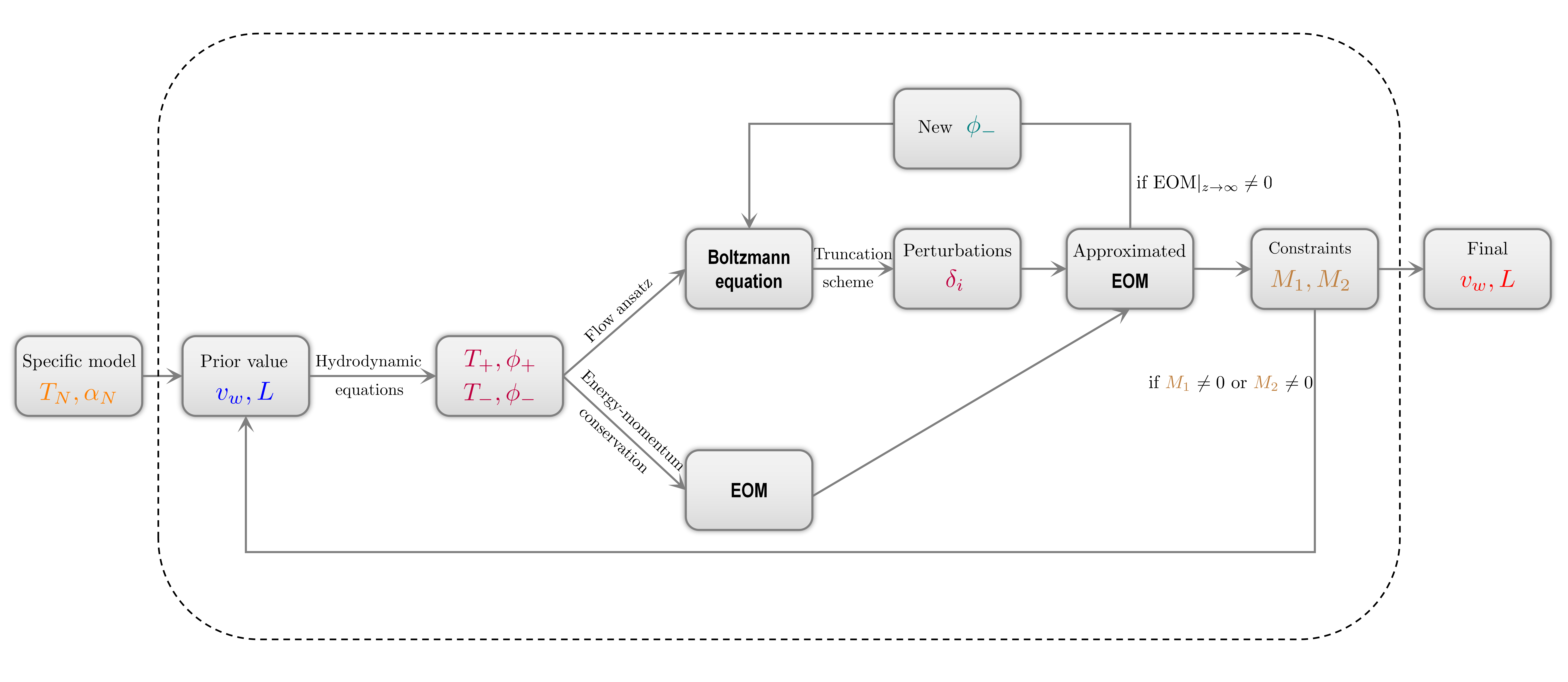
Using the microphysical approach with the recent new methods, for the first time we calculate the bubble wall velocity in the well-motivated inert doublet model (IDM), which could help to greatly reduce the large uncertainties in calculating the phase transition GW and electroweak baryogenesis from the unknown bubble wall velocity. We show the basic procedure to calculate the bubble wall velocity in a given new physics model with a SFOPT in Fig. 1.

This paper is organized as follows. We briefly discuss the IDM and choose the benchmark parameters in Sec. II, and describe the equation of motion for the Higgs background field in Sec. III. Then we derive the hydrodynamic effects in the calculation of bubble wall velocity in Sec. IV. In Sec. V, taking the IDM model as concrete model, we introduce the basic method to calculate the bubble wall velocity. After that, we calculate the collision terms of the IDM in Sec. VI. Therefore, we obtain the final bubble wall velocity in Sec. VII. The conclusion is given in Sec. VIII.

Firstly, we briefly introduce the well-studied IDM, which could improve the naturalness problem and provide a natural DM candidate Barbieri et al. 2006; Lopez Honorez and Yaguna 2010. Meanwhile, the IDM could trigger a SFOPT Chowdhury et al. 2012 in the early Universe around 100 GeV during the electroweak spontaneously symmetry breaking process. Then, one could use the phase transition GW to explore the IDM. However, the GW spectra strongly depend on the bubble wall velocity, which has not been calculated before in the IDM. In this work, we perform detailed calculations on the bubble wall velocity. We begin our discussions from the tree-level scalar potential at zero temperature,

	$\displaystyle V_{0}=$	$\displaystyle\mu^{2}_{1}|\Phi|^{2}+\mu^{2}_{2}|\eta|^{2}+\frac{1}{2}\lambda_{1}|\Phi|^{4}+\frac{1}{2}\lambda_{2}|\eta|^{4}$
		$\displaystyle+\lambda_{3}|\Phi|^{2}|\eta|^{2}+\lambda_{4}|\Phi^{\dagger}\eta|^{2}+\frac{1}{2}\{\lambda_{5}(\Phi^{\dagger}\eta)^{2}+\mathrm{H.c.}\}\,\,,$		(1)

where $\Phi$ is the SM Higgs doublet and $\eta$ represents the inert doublet. The vacuum stability requires $\lambda_{1}>0$, $\lambda_{2}>0$, $\sqrt{\lambda_{1}+\lambda_{2}}+\lambda_{3}>0$, $\lambda_{3}+\lambda_{4}\pm|\lambda_{5}|>0$  Barbieri et al. 2006; Lopez Honorez and Yaguna 2010. At zero temperature, the two doublet scalar fields could be written as

$$\Phi=\begin{pmatrix}G^{+}\\ \frac{1}{\sqrt{2}}(h+v+iG^{0})\end{pmatrix},\ \eta=\begin{pmatrix}H^{+}\\ \frac{1}{\sqrt{2}}(H+iA)\end{pmatrix},$$

(2)

where the mass of SM Higgs boson $h$ is 125 GeV and the vacuum expectation value (VEV) $v=246$ GeV. $G^{\pm}$ and $G^{0}$ are the charged and neutral Nambu-Goldstone bosons respectively. $H$ and $A$ are the $CP$-even and $CP$-odd inert scalars respectively. $H^{\pm}$ are the charged inert scalars. At zero temperature, we show the inert scalar masses beyond the SM

	$\displaystyle\hbox to0.0pt{\hskip 1.89006pt\hbox{$\overline{\hbox{}}$}\hss}{\hbox{$m$}}_{H}^{2}$	$\displaystyle=\mu_{2}^{2}+\frac{1}{2}(\lambda_{3}+\lambda_{4}+\lambda_{5})v^{2},$		(3)
	$\displaystyle\hbox to0.0pt{\hskip 1.89006pt\hbox{$\overline{\hbox{}}$}\hss}{\hbox{$m$}}_{A}^{2}$	$\displaystyle=\mu_{2}^{2}+\frac{1}{2}(\lambda_{3}+\lambda_{4}-\lambda_{5})v^{2},$		(4)
	$\displaystyle\hbox to0.0pt{\hskip 1.89006pt\hbox{$\overline{\hbox{}}$}\hss}{\hbox{$m$}}^{2}_{H^{\pm}}$	$\displaystyle=\mu_{2}^{2}+\frac{1}{2}\lambda_{3}v^{2}\,\,.$		(5)

These new inert scalars could modify $T$ parameter with the deviation $\Delta T$ approximated as

$\displaystyle\Delta T\simeq\frac{1}{6\pi e^{2}v^{2}}(\hbox to0.0pt{\hskip 1.89006pt\hbox{$\overline{\hbox{}}$}\hss}{\hbox{$m$}}_{H^{\pm}}-\hbox to0.0pt{\hskip 1.89006pt\hbox{$\overline{\hbox{}}$}\hss}{\hbox{$m$}}_{H})(\hbox to0.0pt{\hskip 1.89006pt\hbox{$\overline{\hbox{}}$}\hss}{\hbox{$m$}}_{H^{\pm}}-\hbox to0.0pt{\hskip 1.89006pt\hbox{$\overline{\hbox{}}$}\hss}{\hbox{$m$}}_{A})\,\,.$

(6)

From the above expression, there exists a simple and obvious parameter region that $\Delta T\simeq 0$ if we assume $\hbox to0.0pt{\hskip 1.89006pt\hbox{$\overline{\hbox{}}$}\hss}{\hbox{$m$}}_{A}^{2}=\hbox to0.0pt{\hskip 1.89006pt\hbox{$\overline{\hbox{}}$}\hss}{\hbox{$m$}}^{2}_{H^{\pm}}$. This assumption corresponds to $\lambda_{4}=\lambda_{5}<0,~~\lambda_{3}>0$ , and could satisfy all the constraints from electroweak precise measurements, DM direct searches and the collider data Chowdhury et al. 2012. In other words, we assume degenerate $CP$-odd and charged scalar masses

$$\hbox to0.0pt{\hskip 1.89006pt\hbox{$\overline{\hbox{}}$}\hss}{\hbox{$m$}}_{A}^{2}=\hbox to0.0pt{\hskip 1.89006pt\hbox{$\overline{\hbox{}}$}\hss}{\hbox{$m$}}^{2}_{H^{\pm}}=\mu_{2}^{2}+\frac{1}{2}\lambda_{3}v^{2}\,\,.$$

(7)

This makes $\hbox to0.0pt{\hskip 1.89006pt\hbox{$\overline{\hbox{}}$}\hss}{\hbox{$m$}}_{H}^{2}=\mu_{2}^{2}+\lambda_{L}v^{2}$ the lightest particle, which becomes the natural DM candidate Barbieri et al. 2006; Lopez Honorez and Yaguna 2010 with the tiny DM-Higgs boson coupling $\lambda_{L}=(\lambda_{3}+\lambda_{4}+\lambda_{5})/2$. It should be very small to be consistent with the DM direct search. Using the package micrOMEGAs Barducci et al. 2018, we include the resonant effects and require the DM relic abundance Aghanim et al. 2020 $\Omega_{\text{DM}}h^{2}=0.11933\pm 0.00091$. Then we could obtain the constraint Wang et al. 2021b $\lambda_{L}\lesssim 0.003$. These constraints almost reach the blind spots of the IDM, which are difficult for DM direct searches. Future lepton colliders in synergy with phase transition GW might help to explore the DM blind spots Huang and Yu 2018; Wang et al. 2021b. When $\lambda_{3}$, $\lambda_{4}$, $\lambda_{5}$ are $\mathcal{O}(1)$, a SFOPT with associated phase transition GW could be produced Chowdhury et al. 2012; Borah and Cline 2012; Gil et al. 2012; Cline and Kainulainen 2013; AbdusSalam and Chowdhury 2014; Blinov et al. 2015; Cao et al. 2018; Huang and Yu 2018; Laine et al. 2017; Senaha 2019; Huang and Senaha 2019; Kainulainen et al. 2019; Wang et al. 2021b.

When we discuss the phase transition dynamics of the SFOPT, we denote the background of the Higgs field as $\phi$, namely,

$$\Phi=\begin{pmatrix}0\\ \frac{1}{\sqrt{2}}\phi\end{pmatrix}\,\,.$$

(8)

Then we could have the following new field-dependent masses beyond the SM,

	$\displaystyle m_{H}^{2}(\phi)$	$\displaystyle=\mu_{2}^{2}+\frac{1}{2}(\lambda_{3}+\lambda_{4}+\lambda_{5})\phi^{2},$		(9)
	$\displaystyle m_{A}^{2}(\phi)$	$\displaystyle=\mu_{2}^{2}+\frac{1}{2}(\lambda_{3}+\lambda_{4}-\lambda_{5})\phi^{2},$		(10)
	$\displaystyle m^{2}_{H^{\pm}}(\phi)$	$\displaystyle=\mu_{2}^{2}+\frac{1}{2}\lambda_{3}\phi^{2}\,\,.$		(11)

We should obtain the finite-temperature effective potential Niemi et al. 2021; Schicho et al. 2022 after taking the one-loop quantum and thermal corrections with daisy resummation into account. Namely,

$$V_{\text{eff}}(\phi,T)=V_{0}(\phi)+V_{\text{CW}}({\phi})+V_{\text{T}}(\phi,T)\,\,.$$

(12)

The one-loop quantum correction of the potential in the on-shell renormalizaiton scheme is

$$V_{\text{CW}}({\phi},T=0)=\sum_{i}\frac{n_{i}}{64\pi^{2}}\left[{m}_{i}^{4}(\phi)\left(\ln\frac{{m}_{i}^{2}(\phi)}{\hbox to0.0pt{\hskip 1.89006pt\hbox{$\overline{\hbox{}}$}\hss}{\hbox{$m$}}_{i}^{2}}-\frac{3}{2}\right)+2\hbox to0.0pt{\hskip 1.89006pt\hbox{$\overline{\hbox{}}$}\hss}{\hbox{$m$}}_{i}^{2}\bar{m}_{i}^{2}(\phi)\right],$$

(13)

where $n_{i}$ is the degree of freedom for each massive particle $m_{i}(\phi)$. For the daisy resummation, we use the scheme proposed by Dolan and Jackiw Dolan and Jackiw 1974 where one only needs to consider the thermal correction in the thermal function $I_{b}$. Namely, the one-loop thermal correction $V_{\text{T}}$ should be improved as

$$V_{\text{T}}(\phi,T>0)=\sum_{i}n_{i}\frac{T^{4}}{2\pi^{2}}I_{b}\left(\frac{{M}_{i}^{2}}{T^{2}}\right),$$

(14)

where ${M}_{i}^{2}={m}_{i}^{2}(\phi)+\Pi_{i}(T)$ and $I_{b,f}\left(a^{2}\right)=\int_{0}^{\infty}dx~x^{2}\ln\left(1\mp e^{-\sqrt{x^{2}+a^{2}}}\right)$. $\Pi_{i}(T)$ represents the thermal correction for scalar bosons and the longitudinal components of gauge bosons. Scalars with $\mu_{1}^{2}$ and $\mu_{2}^{2}$ appearing in their field-dependent masses can be simply replaced by $\mu_{1}^{2}+\Pi_{\Phi}(T)$ and $\mu_{2}^{2}+\Pi_{\eta}(T)$, respectively, where

	$\displaystyle\Pi_{\Phi}$	$\displaystyle=\frac{T^{2}}{12}\left[3\lambda_{1}+2\lambda_{3}+\lambda_{4}+\frac{3}{4}(3g_{w}^{2}+g_{Y}^{2})+3y_{t}^{2}\right],$		(15)
	$\displaystyle\Pi_{\eta}$	$\displaystyle=\frac{T^{2}}{12}\left[3\lambda_{2}+2\lambda_{3}+\lambda_{4}+\frac{3}{4}(3g_{w}^{2}+g_{Y}^{2})\right].$		(16)

For the gauge bosons, only their longitudinal components need to include the thermal corrections in the thermal function $I_{b}$ as the following:

		$\displaystyle\Pi_{W}(T)=\Pi_{W}^{\Phi}(T)+\Pi_{W}^{\eta}(T)=\left[\frac{11}{6}+\frac{1}{6}\right]g_{w}^{2}T^{2}=2g_{w}^{2}T^{2}\,\,,$		(17)
		$\displaystyle\Pi_{B}(T)=\Pi_{B}^{\Phi}(T)+\Pi_{B}^{\eta}(T)=\left[\frac{11}{6}+\frac{1}{6}\right]g_{Y}^{2}T^{2}=2g_{Y}^{2}T^{2}\,\,,$

where $g_{w}$ and $g_{Y}$ are the gauge coupling of $SU(2)_{L}$ and $U(1)_{Y}$, respectively. Hence, for the longitudinal components of the gauge bosons, their physical masses are eigenvalues of the following matrix

$${M}_{\text{L}}^{2}=\left(\begin{array}[]{cccc}m_{1}^{2}+\Pi_{W}&0&0&0\\ 0&m_{1}^{2}+\Pi_{W}&0&0\\ 0&0&m_{1}^{2}+\Pi_{W}&m_{12}^{2}\\ 0&0&m_{12}^{2}&m_{2}^{2}+\Pi_{B}\\ \end{array}\right)\,\,,$$

(18)

where $m_{1}^{2}=g_{w}^{2}\phi^{2}/4$, $m_{2}^{2}=g_{Y}^{2}\phi^{2}/4$ and $m_{12}^{2}=-g_{w}g_{Y}\phi^{2}/4$.

To focus on the calculation of bubble wall velocity during the SFOPT in the IDM, we simply choose three sets of benchmark model parameters based on our numerical calculations where we use the package micrOMEGAs Barducci et al. 2018 for DM relic abundance, DM direct search, collider constraints Belyaev et al. 2018, and use CosmoTransitions Wainwright 2012 to calculate the phase transition dynamics. Taking all the above discussions into consideration, we choose the following benchmark parameters where $\hbox to0.0pt{\hskip 1.89006pt\hbox{$\overline{\hbox{}}$}\hss}{\hbox{$m$}}_{h}=125$ GeV, $\lambda_{2}=0.2$. Other parameters are shown in Table 1. For these benchmark point sets, the DM relic density, the DM direct search, the collider constraints and condition of the SFOPT could be satisfied simultaneously. We perform detailed calculations of the bubble wall velocity based on Benchmark A and give the final results of bubble wall velocity for Benchmarks B and C.

After bubbles of the broken phase are nucleated, they will expand at a steady bubble wall velocity under some certain circumstances. To obtain the reliable bubble wall velocity in a given new physics model, we firstly need to know the bubble dynamics which are described by the equation of motion (EOM) of the background field for the SFOPT process. We can obtain the EOM by using energy-momentum conservation of the scalar-plasma system. The energy-momentum tensor of the field is

$$T^{\mu\nu}_{\phi}=\partial^{\mu}\phi\partial^{\nu}\phi-g^{\mu\nu}\left(\frac{1}{2}\partial_{\alpha}\phi\partial^{\alpha}\phi-V_{T=0}(\phi)\right)\,\,,$$

(19)

where $\phi$ is the background Higgs field in the IDM, $V_{T=0}(\phi)=V_{0}(\phi)+V_{\rm CW}(\phi)$ is the effective potential at zero temperature. The energy-momentum tensor of the plasma is

$$T_{\mathrm{pl}}^{\mu\nu}=\sum_{i}\int\frac{\mathrm{d}^{3}{p}}{(2\pi)^{3}}\frac{p^{\mu}p^{\nu}}{E_{i}}f_{i}(x,p)\,\,,$$

(20)

where $f_{i}(x,p)$ is the distribution function of the particle and $E_{i}=\sqrt{p^{2}+m_{i}^{2}}$. The sum is over all particle species. Using energy-momentum conservation condition

$$\nabla_{\mu}(T_{\phi}^{\mu\nu}+T_{\rm{pl}}^{\mu\nu})=0\,\,,$$

(21)

we can derive the EOM of the background field Moore and Prokopec 1995b; Moore and Prokopec 1995a; Espinosa et al. 2010; Konstandin et al. 2014,

$$\Box\phi+\frac{\partial V_{T=0}(\phi)}{\partial\phi}+\sum_{i}\frac{dm_{i}^{2}}{d\phi}\int\frac{d^{3}p}{(2\pi)^{3}2E_{i}}f_{i}(x,p)=0\,\,,$$

(22)

During a SFOPT, some massive particles will be in an out-of-equilibrium state near the bubble wall. Hence the distribution function could be approximated as a thermal equilibrium part plus an out-of-equilibrium part, namely,

$$f_{i}\equiv f_{0,i}+\delta f_{i}\,\,.$$

The equilibrium distribution function for fermions and bosons in the plasma frame are given by $f_{0,i}=\frac{1}{\exp(E_{i}/T)\pm 1}$, respectively. The integral of the equilibrium part of the distribution functions gives the thermal-correction part of the effective potential $V_{\rm T}(\phi,\text{T})$. Therefore, the EOM for the background field could be further simplified to

$$\Box\phi+\frac{\partial V_{\rm eff}(\phi,T)}{\partial\phi}+\underbrace{\sum_{i}\frac{dm_{i}^{2}}{d\phi}\int\frac{d^{3}p}{(2\pi)^{3}2E_{i}}\delta f_{i}(x,p)}_{\mathclap{\text{friction term}}}=0\,\,,$$

(23)

where $V_{\text{eff}}(\phi,T)=V_{0}(\phi)+V_{\text{CW}}({\phi})+V_{\text{T}}(\phi,T)$ is the thermal effective potential in a specific model. The second term is the driving term that accelerates the bubble wall. The third term in Eq. (23) behaves as the friction force acting on the bubble wall. We can see that the contributions mainly come from “heavy” particles with non-negligible field-dependent mass. “Heavy” means that the particle could get field-dependent mass comparable with the temperature. Thus, in the IDM, we could only consider the contributions from $t,W^{\pm},Z,A,H^{\pm}$. For the stationary wall, choosing the $-z$ as the propagating direction as shown in Fig. 2, all quantities $Q$ are functions of $z+v_{w}t$, so we can set $z+v_{w}t\rightarrow z$ and hence $\partial_{t}Q\rightarrow v_{w}Q^{\prime}$, $\partial_{z}Q\rightarrow Q^{\prime}$. $v_{w}$ is the bubble wall velocity and prime means derivative with respect to $z$. Then in the plasma frame, the EOM with bubble wall velocity could be further expressed as in Refs. Moore and Prokopec 1995a; Moore and Prokopec 1995b

$$(1-v_{w}^{2})\phi^{\prime\prime}+\frac{\partial V_{\rm eff}(\phi,T)}{\partial\phi}+\sum_{i}\frac{dm_{i}^{2}}{d\phi}\int\frac{d^{3}p}{(2\pi)^{3}2E_{i}}\delta f_{i}(x,p)=0\,\,.$$

(24)

Having the above EOM, we begin to consider the hydrodynamic effects where the temperature might play important roles. For example, Eq. (24) should be evaluated at a specific temperature. Then we should consider the hydrodynamic effects which cause the temperature and velocity profiles varying across the bubble wall Wang et al. 2021a; Espinosa et al. 2010; Leitao and Megevand 2011; Leitao and Megevand 2015; Giese et al. 2020; Giese et al. 2021. This could be seen from the second term of Eq. (24) in the wall frame where we multiply it by $\phi^{\prime}$ and integrate over $z$,

	$\displaystyle\int dz\phi^{\prime}\frac{\partial V_{\rm eff}(\phi,T)}{\partial\phi}$	$\displaystyle=$	$\displaystyle\int dz\frac{dV_{\rm eff}(\phi,T)}{dz}-\int dz\frac{\partial V_{\rm eff}(\phi,T)}{\partial T}\frac{dT}{dz}$		(25)
		$\displaystyle\simeq$	$\displaystyle V_{\rm eff}(\phi_{-},T_{-})-V_{\rm eff}(\phi_{+},T_{+})+\langle s\rangle(T_{-}-T_{+})\,\,,$		(26)

where $V_{\rm eff}(\phi_{-},T_{-})-V_{\rm eff}(\phi_{+},T_{+})$ is the pressure difference that push the bubble wall out. Notice that $\phi_{-}=\phi(z>0)$ and $T_{-}=T(z>0)$ because we let wall move along the negative $z$ direction as shown in Fig. 2 . Entropy density $s(\phi,T)\equiv-\partial V_{\rm eff}(\phi,T)/\partial T$ and it gives non-negligible contribution to the pressure. $\langle s\rangle\simeq\frac{s(\phi_{+},T_{+})+s(\phi_{-},T_{-})}{2}$ is the average entropy density. Notice that the presence of $T_{+}$ here in stead of $T_{N}$ is due to the hydrodynamic heating effects in front of the bubble wall. Besides, as we consider the hydrodynamic effects, temperature in front of the bubble wall $T_{+}$ is usually different from the one behind the wall $T_{-}$. Therefore, it is important to calculate the temperature profile around the bubble wall. All the perturbations are evaluated in front of the wall where $T=T_{+}$.

The energy-momentum tensor of the equilibrium part of plasma and scalar field can be combined in the form of ideal fluid,

$$T_{f}^{\mu\nu}=(e_{f}+p_{f})u^{\mu}u^{\nu}+p_{f}g^{\mu\nu}=\omega_{f}u^{\mu}u^{\nu}+p_{f}g^{\mu\nu}$$

(27)

where $e_{f}$ is the energy density, $p_{f}$ is the pressure and $\omega_{f}$ is the enthalpy of the fluid. $u^{\mu}$ is the fluid four-velocity $u^{\mu}=\gamma(v)(1,\vec{v})$ in the background plasma frame with the Lorentz factor $\gamma(v)=1/\sqrt{1-v^{2}}$.

We can write the hydrodynamic equations in the rest frame of Universe Espinosa et al. 2010,

$\displaystyle\begin{gathered}(\xi-v)\frac{\partial_{\xi}e_{f}}{\omega_{f}}=2\frac{v}{\xi}+\left[1-\gamma^{2}v(\xi-v)\right]\partial_{\xi}v,\\ (1-v\xi)\frac{\partial_{\xi}p_{f}}{\omega_{f}}=\gamma^{2}(\xi-v)\partial_{\xi}v\,\,,\end{gathered}$

where $\xi=r/t$ is the self-similar variable of the above equations and has unit of velocity. $r$ is the distance to the bubble center and $t$ is the time since the bubble nucleation. “Self-similar” means that there is no characteristic length or time scale for one steadily expanding bubble. $v\left(\xi_{w}\right)$ is the fluid velocity at the location of the bubble wall $\xi_{w}$. Notice that $\xi_{w}=v_{w}$.

We can obtain the differential equation for the temperature from Eq. (IV) by using the following identity

$$\frac{\partial p_{f}}{\partial T}=\partial_{\xi}p_{f}\frac{\partial\xi}{\partial T}\,\,,$$

(31)

then the enthalpy can be written as

$$\omega_{f}\equiv T\frac{\partial p_{f}}{\partial T}=T\partial_{\xi}p_{f}\left(\partial_{\xi}T\right)^{-1}\,\,.$$

(32)

Substituting it into Eq. (IV) one obtains

$$\frac{\partial_{\xi}T}{T}=\gamma^{2}\mu\partial_{\xi}v\,\,,$$

(33)

where $\mu(\xi,v)=(\xi-v)/(1-\xi v)$ is Lorentz transformation of the velocity. Given speed of sound in the plasma, $c_{s}^{2}\equiv(dp_{f}/dT)/(de_{f}/dT)$, from Eq. (IV) we can get the equation of the velocity profile,

$$2\frac{v}{\xi}=\gamma^{2}(1-v\xi)\left[\frac{\mu^{2}}{c_{s}^{2}}-1\right]\partial_{\xi}v\,\,.$$

(34)

In order to solve the hydrodynamic fluid equations, one needs to consider the boundary conditions in the system by using the conservation of the energy momentum tensor $\nabla_{\mu}(T_{\phi}^{\mu\nu}+T_{\rm pl}^{\mu\nu})=\nabla_{\mu}T_{f}^{\mu\nu}=0$ across the bubble wall,

$$\omega_{+}\gamma_{+}^{2}v_{+}^{2}+p_{+}=\omega_{-}\gamma_{-}^{2}v_{-}^{2}+p_{-},\quad\omega_{+}\gamma_{+}^{2}v_{+}=\omega_{-}\gamma_{-}^{2}v_{-}\,\,,$$

(35)

which can be transformed as

$$v_{+}v_{-}=\frac{p_{+}-p_{-}}{e_{+}-e_{-}},\quad\frac{v_{+}}{v_{-}}=\frac{e_{-}+p_{+}}{e_{+}+p_{-}}\,\,,$$

(36)

where $+(-)$ means in front of (behind) the bubble wall. These quantities can be estimated by using the so-called bag model. In the bag model, the pressure and the energy density can be written as

$\displaystyle\begin{aligned} &p_{+}=\frac{1}{3}a_{+}T_{+}^{4}-\epsilon_{+},\quad e_{+}=a_{+}T_{+}^{4}+\epsilon_{+},\quad\text{where}\quad\epsilon_{+}\equiv V_{T=0}\left(\phi_{+}\right);\\ &p_{-}=\frac{1}{3}a_{-}T_{-}^{4}-\epsilon_{-},\quad e_{-}=a_{-}T_{-}^{4}+\epsilon_{-},\quad\text{where}\quad\epsilon_{-}\equiv V_{T=0}\left(\phi_{-}\right)\text{. }\end{aligned}$

(37)

Notice that these conditions are derived in the rest frame of the bubble wall. We have pointed out that in order to solve the bubble wall velocity, one important quantity is the temperature in front of the wall $T_{+}$, where massive particles meet the bubble wall. Actually, $v_{+},T_{+}$ are important not only for solving wall velocity but also for calculating electroweak baryogenesis. In bag model we can see the first two terms in Eq. (26),

	$\displaystyle V_{\rm eff}(\phi_{-},T_{-})-V_{\rm eff}(\phi_{+},T_{+})$	$\displaystyle=$	$\displaystyle p_{+}-p_{-}=\epsilon_{-}-\epsilon_{+}+\frac{1}{3}a_{+}T_{+}^{4}-\frac{1}{3}a_{-}T_{-}^{4}$		(38)
		$\displaystyle=$	$\displaystyle\epsilon_{-}-\epsilon_{+}+\frac{1}{3}a_{-}(T_{+}^{4}-T_{-}^{4})+\frac{1}{3}(a_{+}-a_{-})T_{+}^{4}\,\,.$

For weak phase transitions $T_{+}\simeq T_{-}$ the third term is approximately zero and the fourth term accounts for entropy variation which may behave as friction in local equilibrium as discussed in Refs. Konstandin and No 2011; Barroso Mancha et al. 2021; Balaji et al. 2021; Ai et al. 2022; Wang and Yuwen 2022.

Having assumed that the system could be approximated by the bag equation of state, one could obtain a relation between the plasma velocities in front of and behind the bubble wall,

$$v_{+}=\frac{1}{1+\alpha_{+}}\left[\left(\frac{v_{-}}{2}+\frac{1}{6v_{-}}\right)\pm\sqrt{\left(\frac{v_{-}}{2}+\frac{1}{6v_{-}}\right)^{2}+\alpha_{+}^{2}+\frac{2}{3}\alpha_{+}-\frac{1}{3}}\right]\,\,,$$

(39)

where $\alpha_{+}=(\epsilon_{+}-\epsilon_{-})/(a_{+}T_{+}^{4})$ is the phase transition strength. There would be three possible stable solutions to the hydrodynamic equations Steinhardt 1982: 1) Deflagration solution corresponding to the minus sign of above formula has a subsonic wall velocity, and $v_{+}<v_{-}$. In order to fulfill the requirement that the velocity far away from the wall should be zero, there should be a shock front in front of the bubble wall, as we can see in Fig. 2. Note that in this case, the fluid behind the wall is at rest so we have $v_{-}=v_{w}$; 2) For the detonation solution, the wall velocity is supersonic and the fluid in front of the wall is at rest. In this case the solution corresponds to the positive sign of Eq. (39) and we have $v_{+}=v_{w}$; 3)The hybrid expansion occurs when $v_{+}<v_{-}=c_{s}$. This is a hybrid state that there should be a shock front in front of the wall and a rarefaction wave behind the wall.

In this work, we concentrate on deflagration mode where a shock front is formed in front of the bubble wall as shown in Fig. 2. We can clearly see that there exist two different interface boundaries, which lead to discontinuous thermodynamic quantities and two different reference frames. Therefore, we should carefully mention the designated reference frame when we deal with the velocity. For convenience, we denote the fluid velocities as measured with respect to the wall frame as $v_{+}$ if the fluid is in front of the wall and as $v_{-}$ if the fluid is behind the wall. And we denote the fluid velocities as measured with respect to the shock frame as $v_{s+}$ if the fluid is in front of the shock front and as $v_{s-}$ if the fluid is behind the shock front.

For the shock front, the fluid on both sides of it is in the symmetric phase and it has the same matching conditions as bubble wall in Eq. (35), then the velocities on both sides can be written as

$$v_{s+}v_{s-}=\frac{1}{3},\quad\frac{v_{s+}}{v_{s-}}=\frac{T_{s+}^{4}+3T_{s-}^{4}}{T_{s-}^{4}+3T_{s+}^{4}}\,\,.$$

(40)

We use tildes $\tilde{v}_{\pm}$ to refer to fluid velocities in the fluid reference frame. This is also the frame of the universe or the reference frame of the center of the bubble. In this frame the fluid far behind the bubble wall and far ahead of the shock front is at rest. The fluid velocities in wall frame or shock frame and fluid frame are related by Lorentz transformations, i.e.,

$$\tilde{v}_{\pm}=\frac{v_{w}-v_{\pm}}{1-v_{w}v_{\pm}}\,\,,\quad\tilde{v}_{s\pm}=\frac{v_{sh}-v_{s\pm}}{1-v_{\omega}v_{s\pm}}\,\,,$$

(41)

where $v_{w}$ is just the bubble wall velocity, i.e., the relative velocities between the wall and the center of the bubble, $v_{sh}$ is the relative velocity between the shock front and the center of the bubble.

Since we focus on the subsonic bubble wall velocity, we should give a more precise definition of a deflagration. In this case the fluid velocity behind the wall is zero in the fluid frame, i.e,

$$\tilde{v}_{\boldsymbol{-}}=0\quad\longrightarrow\quad v_{w}=v_{\boldsymbol{-}}\,\,.$$

(42)

Similarly, we require that the fluid far away should be at rest as in the presence of the shock front. Then we will get

$$\tilde{v}_{s+}=0\quad\longrightarrow\quad v_{sh}=v_{s+}\,\,.$$

(43)

In order to obtain the fluid velocity and temperature profile in front of the bubble wall, we need to solve their corresponding hydrodynamic equations (33) and (34). Given $\alpha_{+}$ and some value for the wall velocity $v_{w}<c_{s}$, noting we have $\xi_{w}=v_{w}=v_{-}$, the boundary condition for the velocity equation in front of bubble wall is

$$\tilde{v}_{+}\equiv\frac{\xi_{w}-v_{+}}{1-\xi_{w}v_{+}}=v\left(\xi_{w}\right),$$

with $v_{+}$ which is determined by Eq. (39). From Eq. (34), we can see that the solution would have a singularity when $\mu(\xi,v)=c_{s}$. However, the solution will reach the shock front position $\xi_{sh}$ before the singularity. The shock front position satisfies the second boundary condition,

$$\tilde{v}_{s-}\equiv\frac{\xi_{sh}-v_{s-}}{1-\xi_{sh}v_{s-}}=v\left(\xi_{sh}\right)\,\,.$$

(44)

Notice that $\xi_{sh}=v_{sh}=v_{s+}$. However, we still do not know the position of the shock front $\xi_{sh}$. One can use the inverse transformation of Eq. (44) and then substitute it into Eq. (40) which describes the discontinuities of velocities across the shock front, then we will get

$$\mu\left(\xi_{sh},v\left(\xi_{sh}\right)\right)\xi_{sh}=\frac{1}{3}=c_{s}^{2}\,\,,$$

(45)

which determines the position of the shock front. Having the velocity profile, we can substitute it into Eq. (33) to get the temperature profile. The boundary values are the values of the temperature outside the wall $T_{+}$ and the temperature inside the shock front $T_{s-}$. In Fig. 3 we show an illustration of velocity profile and temperature profile where we choose $\alpha_{N}=0.005$. We could integrate Eq. (33) and get

$$\frac{T_{+}}{T_{s-}}=\exp\left[\int_{\xi_{sh}}^{\xi_{w}}d\xi\gamma^{2}\mu\partial_{\xi}v\right]=\exp\left[\int_{\xi_{sh}}^{\xi_{w}}d\xi\frac{2c_{s}^{2}v(\xi-v)}{\xi\left((\xi-v)^{2}-c_{s}^{2}(1-v\xi)^{2}\right)}\right]\,\,.$$

(46)

Notice that the temperature in front of the shock front corresponds to the nucleation temperature of the transition, i.e., $T_{s+}=T_{N}$. Using Eq. (40) and eliminate $v_{s+}$ we can find

$$\frac{T_{s-}^{4}}{T_{N}^{4}}=\frac{T_{s-}^{4}}{T_{s+}^{4}}=\frac{3\left(1-v_{s-}^{2}\right)}{9v_{s-}^{2}-1}\,\,.$$

(47)

Using Eqs. (46) and (47) the temperature in front of the bubble wall $T_{+}$ is related to the nucleation temperature $T_{N}$ as

$$\frac{T_{+}}{T_{N}}=\left(\frac{3\left(1-v_{s-}^{2}\right)}{9v_{s-}^{2}-1}\right)^{1/4}\exp\left[\int_{\xi_{sh}}^{\xi_{w}}d\xi\frac{2c_{s}^{2}v(\xi-v)}{\xi\left((\xi-v)^{2}-c_{s}^{2}(1-v\xi)^{2}\right)}\right]\,\,.$$

(48)

Then we can use

$$\frac{a_{+}T_{+}^{4}}{a_{-}T_{-}^{4}}=\frac{\omega_{+}}{\omega_{-}}\,\,,$$

(49)

to determine the temperature behind the wall $T_{-}$.

In Fig.4 we show an example of the heating effect with $T_{c}=118.3$ GeV and $T_{N}=117.1$ GeV. It can be seen that there is one value of $v_{w}$ at which $T_{+}$ will be larger than $T_{c}$ (However, in reality we think that the $T_{+}$ could not be larger than $T_{c}$. It could only approach $T_{c}$ because when $T_{+}=T_{c}$ the potential difference is almost zero and the wall could not be accelerated anymore.). We can give an approximation of the upper limit of the wall velocity Konstandin and No 2011,

$$v_{w}\simeq\left(\frac{{\rm log}\frac{T_{c}}{T_{N}}}{6\alpha_{c}}\right)^{1/2}.$$

(50)

Actually, the heating effect can effectively be viewed as hydrodynamic backreaction because it effectively reduces the potential difference in front of and behind the wall Konstandin and No 2011; Wang and Yuwen 2022.

Besides heavy particles in the standard model (top quark, $W$ and $Z$ bosons), in IDM we have extra heavy particle species, the $CP$-odd scalar $A$ and two charged scalars $H^{\pm}$ of the inert doublet $\eta$. As we can see in Eqs. (10) and (11), these three scalars have the same coupling such that same field-dependent mass and same interactions. Therefore, in this work one can treat them as the same species $A$. For the same reason, since $W^{\pm}$ and $Z$ have nearly degenerate mass, we can also treat them as the same species $W$. Other massive species that obtain light field-dependent mass should be almost in thermal equilibrium and we can treat them as background.

In order to evaluate the friction term, we adopt the flow ansatz. We must know the out-of-equilibrium distribution part $\delta f$ for each massive particle population. In principle, the distribution function $f$ for the microscopic particles are described by the quantum Liouville equation. However, when the de-Broglie thermal wavelength of particles in the system is smaller than the bubble wall thickness, the Wentzel-Kramers-Brillouin (WKB) condition $p\gg 1/L$ ($p$ is the momentum of concerned particle and $L$ is the bubble wall thickness) is satisfied. Then the background field varies slowly and hence the distribution function for each particle can be approximated by the following Boltzmann equation

$$\frac{d}{dt}f=\left(\frac{\partial}{\partial t}+\dot{z}\frac{\partial}{\partial z}+\dot{p_{z}}\frac{\partial}{\partial p_{z}}\right)f=-C[f]\,\,,$$

(51)

where $\dot{z}=p_{z}/E$ and $\dot{p_{z}}=-\partial_{z}E=-(m^{2})^{\prime}/(2E)$. The distribution function for one species $f$, which deviates from its equilibrium form, can be expressed as

$$f=\frac{1}{e^{(E+\delta)/T}\pm 1}\,\,,$$

(52)

where $+$ is for fermions, $-$ is for bosons, and $\delta$ is the perturbations ($\delta\ll 1$) that can be parametrized as Moore and Prokopec 1995a; Moore and Prokopec 1995b

$$\delta=-\mu-\mu_{bg}-\frac{E}{T}(\delta T+\delta T_{bg})-p_{z}(\delta v+\delta v_{bg})\,\,.$$

(53)

And we take the background chemical potential perturbation as zero Moore and Prokopec 1995a; Moore and Prokopec 1995b. We treat particles and antiparticles as one species neglecting $\mathrm{CP}$ violation.¹¹ 1 Noting that this description is not appropriate for Infrared (IR) excitation with momenta $p\ll T$. These contributions can be important for boson species Moore 2000b; Kozaczuk 2015. $C[f]$ is the collision term, we will discuss the detailed calculations in next section. The collision term and the EOM of the background field are model dependent. Then the Boltzmann equation can be written as

$\displaystyle\begin{aligned} &\left(-f_{0}^{\prime}\right)\left(\frac{p_{z}}{E}\left[\partial_{z}\mu+\frac{E}{T}\partial_{z}\left(\delta T+\delta T_{bg}\right)+p_{z}\partial_{z}\left(\delta v+\delta v_{bg}\right)\right]+\partial_{t}\mu\right.\\ &\left.+\frac{E}{T}\partial_{t}\left(\delta T+\delta T_{bg}\right)+p_{z}\partial_{t}\left(\delta v+\delta v_{bg}\right)\right)+TC[\mu,\delta T,\delta v]=\left(-f_{0}^{\prime}\right)\frac{\partial_{t}\left(m^{2}\right)}{2E}\,\,,\end{aligned}$

(54)

where $f_{0}$ is the equilibrium distribution function and $f_{0}^{\prime}=-\exp(E/T)/[\exp(E/T)\pm 1]^{2}$. It is difficult to solve the full Boltzmann equation. However, one can truncate the full Boltzmann equation with three moments for an approximate solution. The three moments are chosen as $\int d^{3}p/(2\pi)^{3},\int Ed^{3}p/(2\pi)^{2}$, and $\int p_{z}d^{3}p/(2\pi)^{3}$ Moore and Prokopec 1995a; Moore and Prokopec 1995b. Then, after the integration and keeping in mind that $\partial_{t}Q\rightarrow v_{w}Q^{\prime}$, $\partial_{z}Q\rightarrow Q^{\prime}$ for every heavy species $i=t,W,A$, we obtain

	$\displaystyle v_{w}c_{2}^{i}\left(\mu_{i}^{\prime}+\mu_{bg}^{\prime}\right)$	$\displaystyle+v_{w}c_{3}^{i}\left(\delta T_{i}^{\prime}+\delta T_{bg}^{\prime}\right)+\frac{c_{3}^{i}T}{3}\left(\delta v_{i}^{\prime}+\delta v_{bg}^{\prime}\right)+\mu_{i}\Gamma_{\mu 1,i}+\delta T_{i}\Gamma_{T1,i}=\frac{v_{w}c_{1}^{i}}{2T}\left(m_{i}^{2}\right)^{\prime}\,\,,$
	$\displaystyle v_{w}c_{3}^{i}\left(\mu_{i}^{\prime}+\mu_{bg}^{\prime}\right)$	$\displaystyle+v_{w}c_{4}^{i}\left(\delta T_{i}^{\prime}+\delta T_{bg}^{\prime}\right)+\frac{c_{4}^{i}T}{3}\left(\delta v_{i}^{\prime}+\delta v_{bg}^{\prime}\right)+\mu_{i}\Gamma_{\mu 2,i}+\delta T_{i}\Gamma_{T2,i}=\frac{v_{w}c_{2}^{i}}{2T}\left(m_{i}^{2}\right)^{\prime}\,\,,$
	$\displaystyle\frac{c_{3}^{i}}{3}$	$\displaystyle\left(\mu_{i}^{\prime}+\mu_{bg}^{\prime}\right)+\frac{c_{4}^{i}}{3}\left(\delta T_{i}^{\prime}+\delta T_{bg}^{\prime}\right)+\frac{v_{w}c_{4}^{i}T}{3}\left(\delta v_{i}^{\prime}+\delta v_{bg}^{\prime}\right)+\delta v_{i}T\Gamma_{v,i}=0\,\,,$		(55)

with different integration coefficients of the collision term

$\displaystyle\begin{split}&\int\frac{d^{3}p}{(2\pi)^{3}T^{2}}C[f_{i}]=\mu_{i}\Gamma_{\mu 1,i}+\delta T_{i}~\Gamma_{T1,i}\,\,,\\ &\int\frac{d^{3}p}{(2\pi)^{3}T^{3}}EC[f_{i}]=\mu_{i}\Gamma_{\mu 2,i}+\delta T_{i}~\Gamma_{T2,i}\,\,,\\ &\int\frac{d^{3}p}{(2\pi)^{3}T^{3}}p_{z}C[f_{i}]=T\delta v_{i}~\Gamma_{v,i}\,\,.\end{split}$

(56)

In Eqs. (V), the constants $c_{j}^{b/f}$ are defined as

$$c_{j}^{b/f}T^{j+1}=\int E^{j-2}(-f_{0}^{\prime})\frac{d^{3}p}{(2\pi)^{3}}\,\,.$$

(57)

At lowest order in $m/T$, we have

$$c_{1}^{b}=\frac{\log(2T/m_{b})}{2\pi^{2}}\,\,,\quad c_{2}^{b}=\frac{1}{6}\,\,,\quad c_{3}^{b}=\frac{3\zeta(3)}{\pi^{2}}\,\,,\quad c_{4}^{b}=\frac{2\pi^{2}}{15}\,\,,$$

(58)

for bosons, whereas for fermions we have

$$c_{1}^{f}=\frac{\log(2)}{2\pi^{2}}\,\,,\quad c_{2}^{f}=\frac{1}{12}\,\,,\quad c_{3}^{f}=\frac{9\zeta(3)}{4\pi^{2}}\,\,,\quad c_{4}^{f}=\frac{7\pi^{2}}{60}\,\,.$$

(59)

$\zeta(x)$ is the Riemann zeta function.

Eqs. (V) are not enough to solve for six quantities $\mu$, $\delta T$, $\delta v$, $\mu_{bg}$, $\delta T_{bg}$, $\delta v_{bg}$. Therefore, we need three more equations which describe the evolution of the background fluid Moore and Prokopec 1995b. The background fluid is the sum of all light particles which have negligible mass variation across the bubble wall. All light particle species are treated as being at the same temperature $T+\delta T_{bg}$ and same velocity $\delta v_{bg}$ and the annihilation rates are fast enough that the background is in chemical equilibrium $\mu_{bg}=0$. Then we obtain three background equations which have a similar form as the heavy particles in Eqs. (V):

$$\tilde{c}_{4}\left(v_{w}\delta T_{bg}^{\prime}+\frac{\delta v_{bg}^{\prime}}{3}T\right)=N_{t}(\mu_{t}\Gamma_{\mu 2,t}+\delta T_{t}\Gamma_{T2,t})+\sum_{\rm bosons}N_{b}(\mu_{b}\Gamma_{\mu 2,b}+\delta T_{b}\Gamma_{T2,b})\,\,,$$

$$\frac{\tilde{c}_{4}}{3}(\delta T_{bg}^{\prime}+v_{w}T\delta v_{bg}^{\prime})=N_{t}T\delta v_{t}\Gamma_{v,t}+\sum_{\rm bosons}N_{b}T\delta v_{b}\Gamma_{v,b}\,\,,\quad\mu_{bg}=0\,\,,$$

(60)

where we have used the fact that the collision term between massive particle species and light particle species in the fluid equations with opposite sign. Here the heat capacity of the light degrees of freedom $\tilde{c}_{4}=78c_{4}^{f}+19c_{4}^{b}$.