A Generator for Generalized Inverse Gaussian Distributions

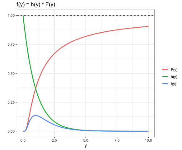
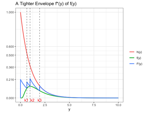
In order to sample $Y$ with the quasi-density $f(y)$, we may choose $h(y)$ as a proposal density and treat $F(y)$ as the acceptance rate. However, as shown in Figure 1, when $y$ is close to 0, which should occur very frequently according to the green curve, the acceptance rate will be close to 0, resulting in an unacceptably high rejection rate. The table 1 shows the acceptance rates for different $(\lambda,\beta)$ if $h(y)$ is chosen as the proposal density. Generally speaking, the acceptance rate would go up as $\beta$ decreases or $|\lambda|$ increases; however, the acceptance rate would be around only 0.5% when $\beta=0.1$ and $\lambda$ = -0.001.

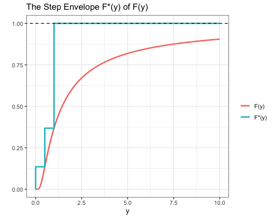
We have to design a much nicer proposal density. Suppose that $\mathbf{k}\in\mathbb{R}^{K}$, $K\geq 1$ is a vector of cutpoints with $0<\mathbf{k}_{i}<\mathbf{k}_{j}<\infty$ for any $i<j$, then we define a step function $F^{*}(y)$ as an envelope of $F(y)$:

with $\mathbf{k}_{0}=0$ and $\mathbf{k}_{K+1}=+\infty$. Since $F^{*}(y)\geq F(y)$ for any $y$, the function $f^{*}(y)=h(y)F^{*}(y)$ is also an envelope of $f(y)=h(y)F(y)$ and thus it can work as a proposal density. In addition, the function $f^{*}(y)$ should be much smaller than the naïve proposal density $h(y)$ as $F^{*}(y)<1$ for any $y<\mathbf{k}_{K}$. For example, in Figure 2(b), the blue curve is the much tighter proposal density $f^{*}(y)$. Compared with the red curve $h(y)$, particularly when $y$ is close to 0, the rejection region is clearly much smaller.

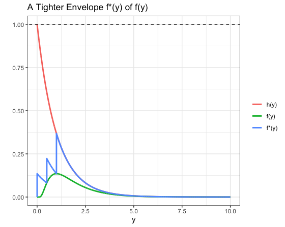
The proposal density $f^{*}(y)$ is also a piecewise function:

For each piece, $F(\mathbf{k}_{i+1})h(y)\cdot\mathbf{1}_{\{\mathbf{k}_{i}\leq y<\mathbf{k}_{i+1}\}}$ is proportional to the density of the truncated exponential distribution $\mathsf{Ex}(\beta/2)\cdot\mathbf{1}_{\{k_{i}\leq y<k_{i+1}\}}$. In addition, since

where

we may sample any variate $Y$ with the quasi-density $f^{*}(y)$ by:

1. Step 1:

   Sample $Z\sim\mathsf{Multinomial}(z_{0},\cdots,z_{K})$;

2. Step 2:

   Sample $Y|Z=z\sim\mathsf{Ex}(\beta/2)\cdot\mathbf{1}_{\{\mathbf{k}_{z}\leq y<\mathbf{k}_{z+1}\}}$.

Furthermore, the rejection rate for any $y\in\mathbb{R}_{+}$ is given by

The Algorithm 2 demonstrates the construction of this piecewise envelope and the corresponding rejection sampling procedure given specific cutoff points $\mathbf{k}$. In addition, the Lemma 3 shows that the random variate $Y$ generated by step 6 in Algorithm 2 follows the distribution $Y|Z=z\sim\mathsf{Ex}(\beta/2)\cdot\mathbf{1}_{\{\mathbf{k}_{z}\leq y<\mathbf{k}_{z+1}\}}$.

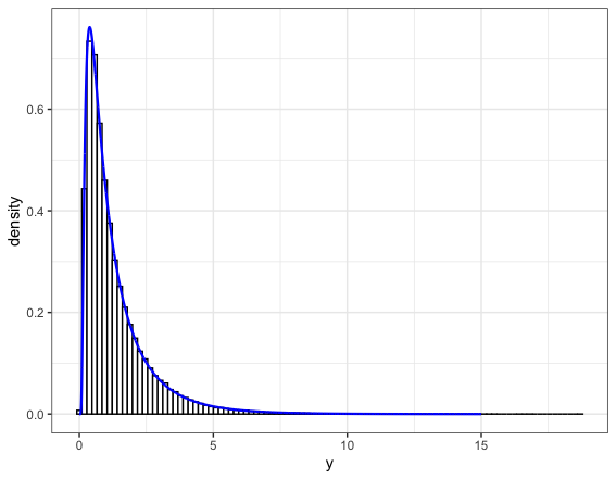
In order to exam the correctness of the rejection sampling procedure in Algorithm 2 when we use $f^{*}(y)$ as the proposal density, we sample from the distribution $\mathcal{GIG}(-0.1,1,1)$ with 100000 draws and compare their summary statistics with the actual density. The Figure 3 shows the histogram of these 10000 draws, which perfectly aligns with the blue actual density curve. In addition, in Table 2, we contrast the actual quantiles and the actual mean which are computed by numerical integrals, with the statistics computed based on the 100000 draws. The simulated ones are similar to the actual ones, which justifies our algorithm 2 as a valid independent GIG variates generator.

Although the tighter envelope $f^{*}(y)$ reduces the rejection rate, its particular construction as well as the resulting rejection rate depends on the choice of cutoff points. In this section, we will develop an algorithm that adaptively chooses the cutoff points given a user-specified rejection rate $\epsilon_{0}$.

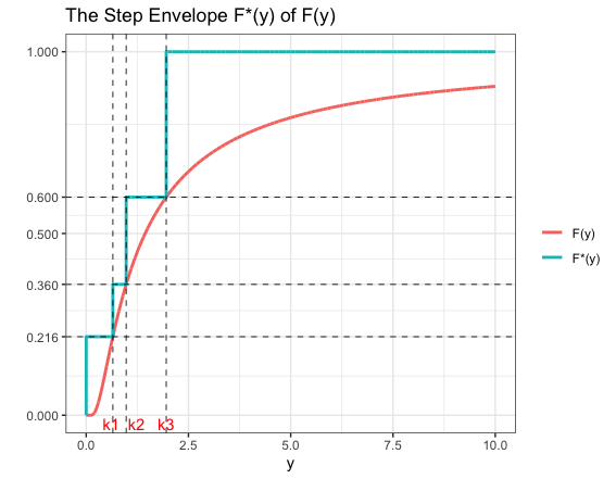
We illustrate our strategy through an example in the Figure 4 where $\lambda=-1$, $\beta=2$ and $\epsilon_{0}=0.8$:

1. Step 1:

   Find the point $\mathbf{k}_{3}$ such that $F(\mathbf{k}_{3})=1-\epsilon_{0}/2$, and set $\mathbf{k}_{3}$ as a cutoff point. Hence for any $y\in[\mathbf{k}_{3},\infty)$, the rejection rate is controlled under $\epsilon_{0}/2$;

2. Step 2:

   Find the point $\mathbf{k}_{2}$ such that $F(\mathbf{k}_{2})=(1-\epsilon_{0}/2)^{2}$, and set $\mathbf{k}_{2}$ as a cutoff point. Hence for any $y\in[\mathbf{k}_{2},\mathbf{k}_{3})$, the rejection rate is also controlled under $\epsilon_{0}/2$;

3. Step 3:

   Find the point $\mathbf{k}_{1}$ such that $F(\mathbf{k}_{1})=(1-\epsilon_{0}/2)^{3}$, and set $\mathbf{k}_{1}$ as a cutoff point. Hence for any $y\in[\mathbf{k}_{1},\mathbf{k}_{2})$, the rejection rate is also controlled under $\epsilon_{0}/2$;

4. Step 4:

   Now we have $z_{0}\leq\epsilon_{0}/2$ (where $z_{0}$ is in the Step 3 of Algorithm 2, the proportion of area of the first piece for $f^{*}(y)$), so the overall rejection rate is less than

   $$\frac{\epsilon_{0}}{2}+(1-\frac{\epsilon_{0}}{2})\cdot\frac{\epsilon_{0}}{2}\leq\epsilon_{0}.$$

The strategy describes a procedure where we start from the density $h(y)$, find a cutoff point $\mathbf{k}^{*}$, pull down the $[0,\mathbf{k}^{*})$ part of the density by the constant $(1-\epsilon_{0}/2)$, and repeat this on a finer resolution. We formulate this procedure into the following algorithm:

We have to show that there must exist a time such that $A_{l}\leq(A_{l}+A_{r})\cdot\epsilon_{0}/2$; in other words, we have to ensure that the Algorithm 3 will terminate itself and the resulting vector has finitely many elements. Now denote the potential new cutoff point $\mathbf{k}_{0}$ at the $n$-th iteration by the sequence $\left\{x_{n}\right\}$ where $x_{n}=F^{-1}((1-\epsilon_{0}/2)^{n})$, then the sequence is monotonically decreasing and $x_{n}\searrow 0$. On the other hand, at the $n$-th iteration, the resulting proposal density is given by

Then the point such that $A_{l}=(A_{l}+A_{r})\cdot\epsilon_{0}/2$ can be represented by a sequence $\left\{y_{n}\right\}$ such that:

Now we show that $\{y_{n}\}$ is a monotonically increasing sequence. Note that

When $x_{n+1}<y_{n}\leq x_{n}$, we have

implying that we must have $y_{n+1}>y_{n}$ such that

Similarly, when $y_{n}\leq x_{n+1}<x_{n}$, we have

implying that we must have $y_{n+1}>y_{n}$ such that

If $x_{1}\leq y_{1}$, then we achieve $A_{l}\leq(A_{l}+A_{r})\cdot\epsilon_{0}/2$ after the first iteration. Otherwise, if $x_{1}>y_{1}$, then since $\left\{x_{n}\right\}$ is monotonically decreasing to 0, and $\left\{y_{n}\right\}$ is monotonically increasing, there must exist $n_{0}>1$ such that $x_{n_{0}}\leq y_{n_{0}}$ so at the $n_{0}$-th iteration we achieve $A_{l}\leq(A_{l}+A_{r})\cdot\epsilon_{0}/2$.

The table 3 shows the simulated acceptance rates for different $(\lambda,\beta)$ combinations given several desired $1-\epsilon_{0}$ using the Algorithm 3. Compared with the first column in Table 1 where we used the naive version, we see that the new algorithm induces a profound improvement in terms of higher acceptance rates. However, we see that the simulated acceptance rates are much higher than the user-specified rates especially when $1-\epsilon_{0}$ is smaller. This implies that our upper bound $\epsilon_{0}/2+(1-\epsilon_{0}/2)\cdot\epsilon_{0}/2$ for the actual overall rejection rate is too conservative and too loose, and resources are wasted to set up more cutoff points than necessary. One possible ad-hoc strategy in practice is to feed in $2\epsilon_{0}$ instead of $\epsilon_{0}$ to Algorithm 3, and the simulation results are shown in Table 4. We see that the simulated acceptance rate is still larger than desired but not that large here.

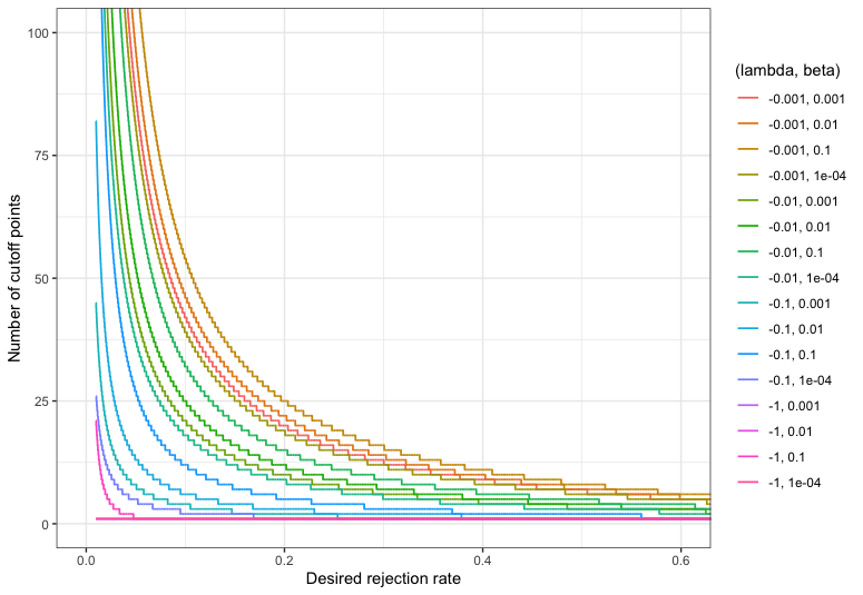
In addition to the control of acceptance rates, the Algorithm 3 (and its ad-hoc version) also provides a tool to see the trade-off between the rejection rate and the number of cutoff points. In Figure 5, we divide the rejection rate range $(0,1]$ into 50000 equispaced intervals and compute the corresponding number of cutoff points for 16 different $\mathcal{GIG}(\lambda,\beta)$. Based on the plot, we see that the number of cutoff points is a monotonically decreasing function of the desired rejection rate $\epsilon_{0}$. Particularly, when $\epsilon_{0}\rightarrow 1$, the number of cutoff points goes to 0; whereas when $\epsilon_{0}\rightarrow 0$, then number of cutoff points goes to infinity.

It is not surprising that a lower desired rejection rate would lead to more cutoff points, as intuitively it may take more iterations for each piece of the proposal density to be tighter to $f(y)$. On the other hand, a smaller number of cutoff points may lead to a higher overall rejection rate, and in the extreme case when we have no cutoff points the Algorithm 3 degenerates to the native version.

We have investigated the strategy to choose cutoff points when the rejection rate is given; however, on the other end of the trade-off spectrum, it is also critical to develop a strategy that adaptively chooses cutoff points given the desired number of points. We hope that the specific cutoff points $\mathbf{k}$ we obtain given the number of cutoff points $K$, can be consistent with those cutoff points $\mathbf{k}^{\prime}$ given the desired rejection rate $\epsilon_{0}$. In other words, the points $\mathbf{k}$ should achieve similar guaranteed acceptance rates as those $\mathbf{k}^{\prime}$ such that $|\mathbf{k}|=|\mathbf{k}^{\prime}|$. Similarly, the points $\mathbf{k}^{\prime}$ should have approximately the same length as that of $\mathbf{k}$ if $\mathbf{k}$ and $\mathbf{k}^{\prime}$ enjoy similar rejection rate bounds.

Fortunately, the number of cutoff points $K$ is a monotonically decreasing function of the desired rejection rate $\epsilon_{0}$ as shown in the last section. We call this function $K=K^{*}(\epsilon_{0})$. With this trade-off we may take advantage of binary search to find

and the corresponding exact cutoff points (see Algorithm 4).

The Table 5 shows the simulated acceptance rates when the numbers of cutoff points are pre-specified. Note that for any cell in this table the actual number of cutoff points coincides with the corresponding desired number. Consequently, it is clear that with more cutoff points the actual rejection rate decreases, which again reveals their trade-off relationship.

Note that the Algorithm 4 should be much less efficient than the Algorithm 3, since the function find.cutoff.under.rej.rate(), in general, need to be called for multiple times during the procedure of binary search in Algorithm 4 when we make use of the non-increasing function $K=K^{*}(\epsilon_{0})$. Sometimes people may need to compare the time complexity of algorithms under different settings by specifying a benchmark, such as a common desired rejection rate (an upper bound for the rejection rate) or a common number of cutoff points. Since it is efficient to evaluate the function $K=K^{*}(\epsilon_{0})$ given $\epsilon_{0}$ while rather inefficient to find the pre-image of $K^{*}(\cdot)$ given $K$, we should always use a common desired rejection rate $\epsilon_{0}$.

Why do we design the Algorithm 4, then, if the binary search procedure is so time-costly? From Figure 5, we see that when the desired rejection rate $\epsilon_{0}$ is close to 0, a tiny shift downward in $\epsilon_{0}$ would result in an extremely large increment in the number of cutoff points. In this case, the time spent on setting up cutoff points might exceed the time saved from a small rejection rate so we have to be careful in terms of controlling the most time-consuming part. In summary, under the setting when the number of cutoff points is significantly effective on the running time and it is affordable to run the binary search, we may use the function find.cutoff.under.fix.num() before the actual sampling procedure.

Additionally, there are cases when we need to compare our algorithm with other existing procedures where the actual rejection rate (or rejection constant) is chosen as a comparing metric. It would make no sense if we control the comparing metric in advance, and thus choosing a common number of cutoff points for each parameter is much more fair for the comparisons if the time complexity is not a major concern.

In this section, we are going to delve into the time complexity of the combined algorithm to explore the relationship between running time and the user-specified tuple $(\epsilon_{0},K)$.

The Algorithm 5 can be decomposed in the following way:

1. Part 1:

   The line 1 to line 5 and the line 11 take around constant time.

2. Part 2:

   The line 6 to line 10 are associated with the number of cutoff points. In particular, if we find the cutoff points given the desired rejection rate (through the function find.cutoff.under.rej.rate() in Algorithm 3), then the time spent in this part can be expressed as $T_{1}\cdot K^{*}(\epsilon_{0})$ where $T_{1}$ is the average time of looking for each cutoff point, and $K^{*}(\epsilon_{0})$ is the resulting number of cutoff points. Note that the actual value of $T_{1}$ depends on specific machine settings but the time used for each cutoff point should remain similar.

3. Part 3:

   The line 12 is associated with the rejection sampling procedure. Particularly, inside the Algorithm 2 (denoted by rejection.sampling()) the line 1 is of constant time. Additionally, the time spent on line 2 and line 3 can be expressed as $T_{2}\cdot K^{*}(\epsilon_{0})$ where $T_{2}$ is the average time on setting up each point. The time spent on line 4 to line 13 can be expressed as $T_{3}\cdot N^{\prime}$ where $T_{3}$ is the average time of drawing one variate from the proposal density, and $N^{\prime}$ is the total number of draws (among which some are accepted and some are rejected). Similarly as above, the actual values of $T_{2}$ and $T_{3}$ depend on specific machine settings but the time used for each draw should remain similar.

4. Part 4:

   The line 13 to 17 are of linear time of $N$. In other words, the time spent on this part can be expressed as $T_{4}\cdot N$, which solely depends on the number of variates. Still, the acutal value of $T_{4}$ dependes on specific machine settings but the time used for post-processing each variate should remain similar.

Now we ignore the constant time consumption and consider the average generating time for each variate:

where we use the desired rejection rate to approximate the actual rejection rate $1-N/N^{\prime}$. Note that $K^{*}(\epsilon_{0})$ is a decreasing function of $\epsilon_{0}$ so the first term is a decreasing function of $\epsilon_{0}$ as well; however, the second term is an increasing function of $\epsilon_{0}$. When $\epsilon_{0}$ goes close to 0 or 1 the average time tends to infinity, implying that there should be a minimum point in between such that $T_{\rm total}/N$ attains its minimum when $N$ is fixed.

We may also see the effect of varying $N$ when $\epsilon_{0}$ is fixed. When $N$ is small, for example when we are trying to draw only one sample for each iteration of a Gibbs sampler, the part $(T_{1}+T_{2})\cdot K^{*}(\epsilon_{0})$ representing the cutoff-point-processing time might dominate the average generating time particularly when $\epsilon_{0}$ is small. However, when $N$ becomes large, for example when we are trying to obtain Monte Carlo estimates through drawing a large sample from GIG, the part $T_{3}/(1-\epsilon_{0})+T_{4}$ will ultimately dominate the average generating time.

In summary, given the same desired rejection rate $\epsilon_{0}$, a large sample size should be able to save the average time spent on pre-processing cutoff points as the pre-processing procedure need not be repeated for each subsequent iteration of rejection sampling.

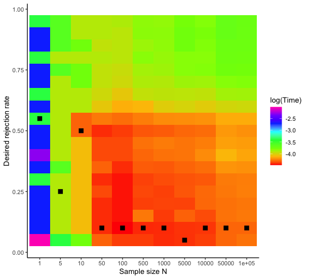
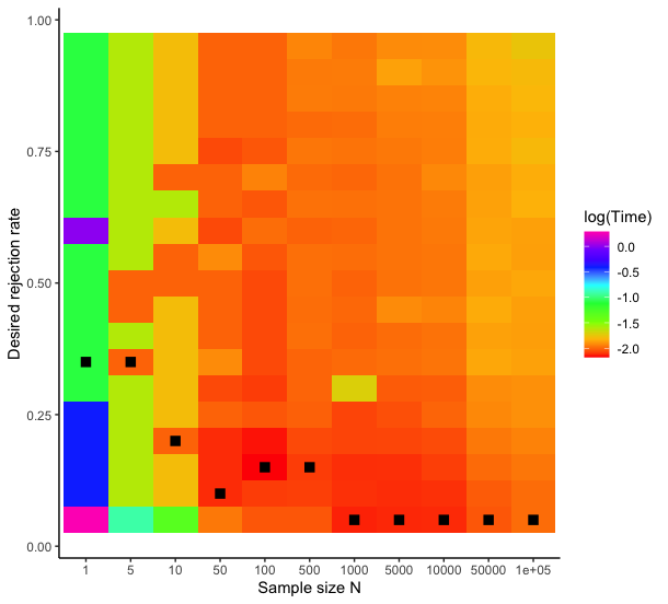
The Figure 6 shows simulated average generating time $T_{\rm total}/N$ under different desired rejection rates $\epsilon_{0}$ and different samples sizes $N$, where the black squares represent the minimal values in each column. The value in each cell is computed as the average value over 30 replicates. Generally speaking, for a small sample size ($N\leq 10$), the best desired rejection rate $\epsilon_{0}$ which induces the shortest average running time would be around 0.5; while for a large sample size ($N>1000$), the corresponding best desired rejection rate $\epsilon_{0}$ would be around 0.05 to 0.1. In addition, the average running time given $\epsilon_{0}$ is roughly decreasing with increasing $N$. Particularly, a larger sample size $N$ and a smaller $\epsilon_{0}$ would lead to an overall shorter running time: the smallest values cluster in the right bottom corner of the plots.

These plots again show the trade-off between rejection rate and number of cutoff points. When we need only one variate, it is not worthwhile to spend too much time on setting up cutoff points even though it may result in higher rejection rate. On the other hand, when we need a large sample, the benefits of low rejection rate would exceed the average loss on the pre-processing procedure that deals with cutoff points so a low rejection rate is the best option.

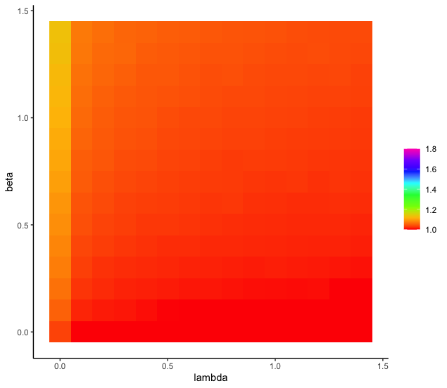
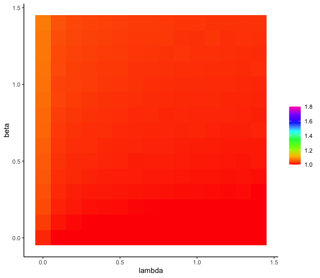
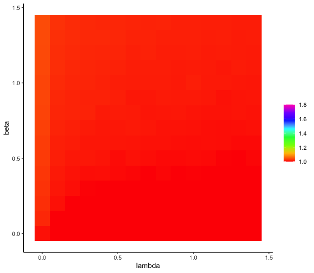
Previously we provided time complexity analysis and performed running time comparisons between different scenarios for our own approach. Nevertheless, it is always a concern that how our approach would outperform other existing algorithms. As we mentioned in Section 1, Hörmann and Leydold 2014 improved a commonly used ratio-of-uniforms method for generating GIG variates and provide their uniformly bounded rejection constants for the particularly interested range $\lambda\in(0,1.5]$ and $\beta\in(0,1.5]$. The rejection constant can be estimated by #(variates draw from proposal density) / #(variates being accepted).

In order to align with their results, we have to treat the rejection constant as the metric as well. Note that in our approach, the rejection constants can be upper bounded by $1/(1-\epsilon_{0})$ and hence are automatically controlled if we specify the desired rejection rate $\epsilon_{0}$, although might at the price of extremely large number of cutoff points. Another strategy of comparison, with the goal of a fair game, is to fix several different numbers of cutoff points and then compare the rejection constants.

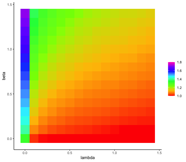
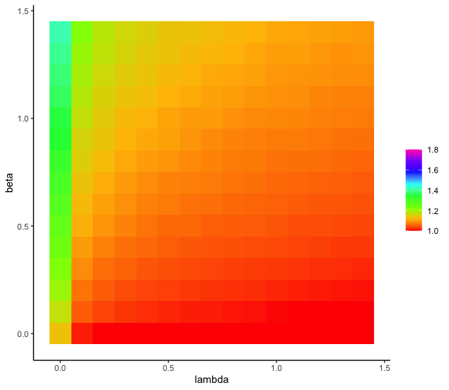
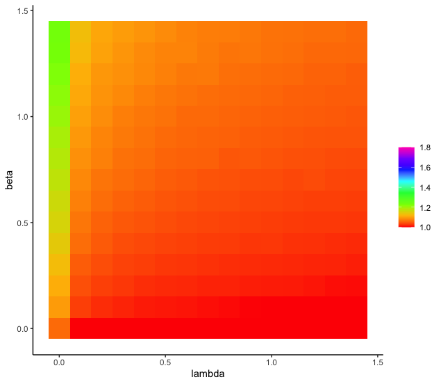
The Figure 7 shows the estimated rejection constants when we sample 50000 independent variates for each parameter $(\lambda,\beta)$. One immediate observation is that the sampling procedure is particularly harder when $\lambda$ is close to 0, where the rejection constants become abruptly large. In addition, higher $\beta$ leads to larger rejection constant while higher $\lambda$ leads to lower rejection constant. Finally, as the number of cutoff points increase, the rejection constants are decreasing. Specifically, the rejection constants are uniformly bounded and smaller than the results in Hörmann and Leydold 2014 when $K\geq 20$.

References

- Abramowitz and Stegun (1948) Milton Abramowitz and Irene A Stegun. Handbook of mathematical functions with formulas, graphs, and mathematical tables, volume 55. US Government printing office, 1948.
- Atkinson (1982) AC Atkinson. The simulation of generalized inverse gaussian and hyperbolic random variables. SIAM Journal on Scientific and Statistical Computing, 3(4):502–515, 1982.
- Barndorff-Nielsen (1977) Ole Barndorff-Nielsen. Exponentially decreasing distributions for the logarithm of particle size. Proceedings of the Royal Society of London. A. Mathematical and Physical Sciences, 353(1674):401–419, 1977.
- Barndorff-Nielsen (1978) Ole Barndorff-Nielsen. Hyperbolic distributions and distributions on hyperbolae. Scandinavian Journal of statistics, pages 151–157, 1978.
- Barndorff-Nielsen and Halgreen (1977) Ole Barndorff-Nielsen and Christian Halgreen. Infinite divisibility of the hyperbolic and generalized inverse gaussian distributions. Zeitschrift für Wahrscheinlichkeitstheorie und verwandte Gebiete, 38(4):309–311, 1977.
- Barndorff-Nielsen et al. (1978) Ole Barndorff-Nielsen, Preben Blæsild, and Christian Halgreen. First hitting time models for the generalized inverse gaussian distribution. Stochastic Processes and their Applications, 7(1):49–54, 1978.
- Dagpunar (2007) John Selim Dagpunar. Simulation and Monte Carlo: With applications in finance and MCMC. John Wiley & Sons, 2007.
- Dagpunar (1989) JS Dagpunar. An easily implemented generalised inverse gaussian generator. Communications in Statistics-Simulation and Computation, 18(2):703–710, 1989.
- Halphen (1941) E Halphen. Sur un nouveau type de courbe de fréquence. Comptes Rendus de l’Académie des Sciences, 213:633–635, 1941.
- Hörmann and Leydold (2014) Wolfgang Hörmann and Josef Leydold. Generating generalized inverse gaussian random variates. Statistics and Computing, 24(4):547–557, 2014.
- Jørgensen (1982) Bent Jørgensen. Statistical properties of the generalized inverse Gaussian distribution. Number 9 in Lecture notes in statistics. Springer, New York, 1982.
- Leydold and Hörmann (2011) Josef Leydold and Wolfgang Hörmann. Generating generalized inverse gaussian random variates by fast inversion. Computational statistics & data analysis, 55(1):213–217, 2011.
- McNeil et al. (2015) Alexander J McNeil, Rüdiger Frey, and Paul Embrechts. Quantitative risk management: concepts, techniques and tools-revised edition. Princeton university press, 2015.
- Seshadri (2012) Venkata Seshadri. The inverse Gaussian distribution: statistical theory and applications, volume 137. Springer Science & Business Media, 2012.