The Euclidean Space is Evil: Hyperbolic Attribute Editing
for Few-shot Image Generation
Abstract
Few-shot image generation is a challenging task since it aims to generate diverse new images for an unseen category with only a few images. Existing methods suffer from the trade-off between the quality and diversity of generated images. To tackle this problem, we propose Hyperbolic Attribute Editing (HAE), a simple yet effective method. Unlike other methods that work in Euclidean space, HAE captures the hierarchy among images using data from seen categories in hyperbolic space. Given a well-trained HAE, images of unseen categories can be generated by moving the latent code of a given image toward any meaningful directions in the Poincaré disk with a fixing radius. Most importantly, the hyperbolic space allows us to control the semantic diversity of the generated images by setting different radii in the disk. Extensive experiments and visualizations demonstrate that HAE is capable of not only generating images with promising quality and diversity using limited data but achieving a highly controllable and interpretable editing process. Code is available at https://github.com/lingxiao-li/HAE.
1 Introduction
Due to the persistent development of deep learning, the task of image generation has received significant research attention in recent years. Specifically, the Generative Adversarial Networks (GANs) Goodfellow14 and its variants (e.g., StyleGANv2 Karras20) have succeeded in generating high-fidelity and realistic images, requiring a large number of high-quality data for model training. However, considering the long-tail distribution and data imbalance widely exists among different image categories Hong20F2, it is difficult for GANs to be trained on categories with sufficient training images to generate new realistic and diverse images for a category with only a few images. This task is referred to as few-shot image generation Clouâtre19; Hong20; Hong20F2; Hong20Match; Hong22; Hong22Delta; Ding22. A variety of tasks can benefit from improvements in few-shot image generation, for instance, low-data detection Fu19 and few-shot classification Sung18; Vinyals16.

In general, existing GAN-based few-shot image generation mechanisms can be classified into three categories. Transfer-based methods Clouâtre19; Liang20 introduce meta-learning or domain adaptation on GANs to generate new images by enforcing knowledge transfer among categories. Fusion-based methods Bartunov18; Gu21; Hong20F2; Hong20Match perform feature fusion of multiple input images in a feature space and generate images via decoding the fused features back to image space. However, the output is still highly similar to the source images. Transformation-based methods Antoniou17; Hong22; Hong22Delta; Ding22 find intra-category transformations or inject random perturbations to conditional unseen category samples to generate images without tedious fine-tuning. By representing the images in the Euclidean feature space, the above learning mechanisms tend to be over-complicated, and the generated images are often collapsed due to limited diversity.
Similar to the ubiquity of hierarchies in language Nickel17; Tifrea19; Dhingra18, the semantic hierarchy is also common in images Khrulkov21; Cui23. As Fig. 1 shows, the semantic hierarchies constructed in the language domain can be instantiated with visual images. From the visual perspective, an image can be regarded as a collection of attributes of multiple levels. High-level attributes, a.k.a. category-relevant attributes, define the category of an image, such as the shape and color of an animal Ding22. For instance, in the middle row of Fig. 1, changing the high-level attributes of the given image of a Shih-Tzu dog, the category can be changed to a Rhodesian Ridgeback Dog. While the low-level or fine-grained attributes, including expressions, postures, etc., that vary within the category as shown at the bottom of Fig. 1, are called category-irrelevant attributes. Therefore, an image can also be viewed as a descendant of another image with the same category-relevant attributes by adding fine-grained category-irrelevant attributes to its parent image. To edit the visual attributes for high-quality image generation, it is crucial to capture the attribute hierarchy within the large image data corpus and find a good representation space. Ideally, we aim to construct a hierarchical visual representation in a latent space that allows us to change the category of an image by moving the latent code in a category-relevant direction, and perform few-shot image generation by moving the code in a category-irrelevant direction.
Unfortunately, the Euclidean space and its corresponding distance metrics used by existing GAN-based methods can not facilitate the hierarchical attribute representation, thus the design of complicated attribute disentangling and editing mechanisms seems to be crucial for the generation quality. Inspired by the application of hyperbolic space in images Khrulkov21 and videos Surís21, we found that the metrics introduced in hyperbolic geometry can naturally and compactly encode hierarchical structures. Unlike the general affine spaces, e.g., the Euclidean space, hyperbolic spaces can be viewed as the continuous analog of a tree since tree-like graphs can be embedded in finite-dimension with minimal distortion Nickel17. This property of hyperbolic space provides continuous and up to infinite semantic levels for attribute editing, allowing us to robustly generate diverse images with only a few images from unseen categories with simple operations.
Based on the above findings, we propose a simple but effective Hyperbolic Attribute Editing (HAE) method for few-shot image generation. Our method is based on the observation that hierarchical latent code manipulation can be easily implemented in Hyperbolic space. The core of HAE is mapping the latent vectors from the Euclidean space to a hyperbolic space . We minimize a supervised classification loss function to ensure the images are hierarchically embedded in hyperbolic space. Once we capture the attribute hierarchy among images, we can generate new images of unseen categories by moving the latent code from one leaf to another with the same parents by fixing the radius. Most importantly, the hyperbolic space allows us to control the semantic diversity of generated images by setting different radii in the Poincaré disk. Those operations can well facilitate continually hierarchical attribute editing in hyperbolic space for flexible few-shot image generation with both quality and diversity.
Our contributions can be summarized as follows:
- •
We propose a simple yet effective method for few-shot image generation, i.e., hyperbolic attribute editing. In order to capture the hierarchy among images, we use hyperbolic space as the latent space. To the best of our knowledge, HAE is the first attempt to use hyperbolic latent spaces for few-shot image generation.
- •
We show that in our designed hyperbolic latent space, the semantic hierarchical attribute relations among images can be reflected by their distances to the center of the Poincaré disk.
- •
Extensive experiments and visualization suggest that HAE achieves stable few-shot image generation with state-of-the-art quality and diversity. Unlike other few-shot image generation methods, HAE allows us to generate images with better control of diversity by changing the semantic levels of attributes we want to edit.

2 Related Work
Few-shot image generation. Recently, diverse methods have been proposed for few-shot image generation. The transfer-based methods Clouâtre19; Liang20 which introduce meta-learning or domain adaptation on GANs can hardly generate realistic images. While fusion-based methods that fuse the features by matching the random vector with the conditional images Hong20Match or formulating the problem as a conditional generating task Gu21; Hong20F2 suffer from the limited diversity of generated images. Furthermore, transformation-based methods Antoniou17; Hong22; Hong22Delta; Ding22 can generate images with only one conditional image by focusing on either capturing the cross-category or intra-category transformations by injecting random perturbations Antoniou17. Nevertheless, the transformation captured by those methods is not very consistent. Ding et al. Ding22; Ding23 propose the “editing-based” perspective, the intra-category transformation can be modeled as category-irrelevant image editing based on one sample instead of pairs of samples. Most recently, Zhu et al. Zhu22 fine-tune powerful diffusion models (DMs) Ho20 pre-trained on large source domains on limited target data to generate diverse and high quality images. DMs outperform GANs Goodfellow14 on sample quality with a more controllable training process at the cost less flexibility and editability, since they denoise images in the image space rather than operate in the latent space. Furthermore, the inference process of DMs is much slower than GANs Song21DDIM.
Hyperbolic Embedding. The use of hyperbolic space in deep learning Nickel17; Nickel18; Tifrea19; Surís21; Khrulkov21 is a pioneering work in recent years. It was first used in natural language processing for hierarchical language representation Nickel17; Nickel18; Tifrea19. The Riemannian optimization algorithms are used to optimize models in hyperbolic space Bécigneul19; Bonnabel13. As hyperbolic space is successfully applied to represent hierarchical data, Ganea et al. Ganea18 derives hyperbolic versions of tools in neural networks including multinomial logistic regression, feed-forward, and recurrent neural networks. Following this, hyperbolic geometry is used in image Khrulkov21, video Surís21, and graph data Chami19; Park21. Most recently, Lazcano et al Lazcano21 shows that hyperbolic space outperforms traditional Euclidean space in image generation using HGAN. However, the hierarchy and controllability of hyperbolic space remain uninvestigated in HGAN, as the generator is still governed by Gaussian samples in Euclidean space.
Latent Code Manipulation. It has been shown that the latent spaces of GANs are able to encode rich semantic information Goetschalckx19; Jahanian20; Shen20. One of the popular approaches is finding linear directions corresponding to changes in a given binary labeled attributes, which might be difficult to obtain for new datasets and could require manual labeling effort Shen20; Goetschalckx19; Denton19. Others Cherepkov21; Voynov20; Lu20; Härkönen20; Choi22 try to find semantic directions in an unsupervised manner. For instance, PCA is applied in the latent space to create interpretable controls for synthesizing images Härkönen20; Choi22. Most recent works Eliezer21; Shen21 directly compute in the close form to find the meaningful semantic direction without training and optimization. In comparison, our work HAE focuses on attributes in different semantic levels in the latent space rather than trying hard to find disentangled interpretable directions as previous works.
3 Method
The overall framework of HAE is shown in Fig. 2, we first give a detailed explanation of getting the hierarchical representations in the hyperbolic space, and then we introduce the framework of HAE and explain the loss functions.
3.1 Hierarchical Representation
The major issue of our study is how to obtain the hierarchical representation from real images to facilitate editing in different semantic levels, as illustrated in Fig. 1. Therefore, hyperbolic space is introduced as the latent space to achieve this goal.
Unlike Euclidean spaces with their zero curvature and spherical spaces with their positive curvature, hyperbolic spaces with negative curvature have been shown that it is more appropriate for learning hierarchical representation Nickel17; Nickel18. Informally, hyperbolic space can be viewed as a continuous analogy of trees Nickel17. One important feature of hyperbolic space is that the length grows exponentially with its radius while linearly in Euclidean space. This property allows hyperbolic space to be naturally compatible with hierarchical data Gromov87 including text, images, videos, etc.
The -dimensional hyperbolic space can be formally defined as a homogeneous, simply connected -dimensional Riemannian manifold, denoted as with constant negative sectional curvature11 1 The curvature of the hyperbolic space is set as in this work.. We choose to work in the Poincaré disk from five isometric models of hyperbolic space defined in Cannon97 since it is commonly used in gradient-based learning Nickel17; Ganea18; Nickel18; Tifrea19; Surís21; Khrulkov21. The Poincaré disk model is defined by the manifold equipped with the following Riemannian metric:
| (1) |
where , and is the Euclidean metric tensor . The induced distance between two points can be defined by:
| (2) |

Recall that a geodesic is a locally minimized-length curve between two points. In the hyperboloid model, the geodesic can be defined as the curve created by intersecting the plane defined by two points and the origin with the hyperboloid Lee13. Thus, the mean of two latent codes in hyperbolic space locates at the mid-point of the geodesic that is closer to the origin. This is the key desired feature of hyperbolic space, i.e., the mean between two leaf embeddings is not another leaf embedding, but the hierarchical parent of them Surís21. This feature allows us to generate new images by moving the latent code from one leaf to another with the same parents. We can also change the semantic levels of attributes by determining how abstract their parent is.
This unique property is visualized in Fig. 3 on a 2-D Poincaré disk. The image embedding near the edge of the ball (with a large radius) represents a more fine-grained image while the embedding near the center (which has a smaller radius) represents an image with abstract features (an average face).
Although the hyperbolic space shares similar features with trees, it is continuous. In other words, there is no fixed number of hierarchy levels. Instead, there is a continuum from very fine-grained (near the edge of Poincaré disk) to very abstract (near the origin).
3.2 Network Architecture
Although we aim to embed and edit real images in hyperbolic space, the whole network does not need to be implemented in a hyperbolic manner. Instead, we can take advantage of the number of existing GAN inversion models and optimization algorithms that have been fine-tuned for Euclidean space.
To achieve image editing, we need to embed the image back into the latent space. In particular, we select pSp Richardson21 as the backbone of HAE to encode images to the -space of StyleGAN2 Karras20:
| (3) |
where is the corresponding latent vector of in the -space.
To manipulate latent code in hyperbolic space, we need to define a bijective map from to to map Euclidean vectors to the hyperbolic space and vice versa. A manifold is a differentiable topological space that locally resembles the Euclidean space Lee06; Lee13. For , one can define the tangent space of at as the first order linear approximation of around . Therefore, this bijective map can be performed by exponential and logarithmic maps. Specifically, the exponential map , maps from the tangent spaces into the manifold. While the logarithmic map is the reverse map of the exponential map.

We use exponential and logarithmic maps at origin 0 for the transformation between the Euclidean and hyperbolic representations. After getting in the -space, we first use a Multi-layer Perceptron (MLP) encoder to reduce the dimension of latent vectors in Euclidean space. Then we apply an exponential map to project the Euclidean latent code to hyperbolic space. After that, we use the hyperbolic feed-forward layer as Ganea18 to obtain the final hierarchical representation as shown in Fig. 2:
| (4) |
where is the Möbius translation of feed-forward layer as the map from to , denoted as Möbius linear layer.
Finally, the hyperbolic representation needs to be projected back to the -space of StyleGAN2. In practice, this is achieved by applying a logarithmic map followed by an MLP decoder:
| (5) |
and will be fed into a pre-trained StyleGAN2’s generator to reconstruct the image .
3.3 Loss Function
The loss function of HAE consists of two parts: the Hyperbolic loss ensures to get the hierarchical representation in the hyperbolic space and the reconstruction loss guarantees the quality of reconstruction images.
Hyperbolic Loss. To learn the semantic hierarchical representation of real images in hyperbolic space, we minimize the distance between latent codes of images with similar categories and attributes while pushing away the latent codes from different categories. We choose the supervised approach to achieve this. In order to perform multi-class classification on the Poincaré disk defined in Section 3.1, one needs to generalize multinomial logistic regression (MLR) to the Poincaré disk defined in Ganea18. An extra linear layer needs to be trained for the classification and the softmax probability can be computed as: Given classes and :
| (6) | ||||
where denotes the Möbius addition defined in Khrulkov21 with fixed sectional curvature of the space, denoted by .
After getting the softmax result for each class, one can use negative log-likelihood loss (NLL Loss) to calculate the hyperbolic loss:
| (7) |
where is the batch size and is the probability predicted by the model for the correct class.
As mentioned in Section 3.1, the distance between points grows exponentially with their radius in the Poincaré disk. In order to minimize Eq. 7, the latent codes of fine-grained images will be pushed to the edge of the ball to maximize the distances between different categories while the embedding of abstract images (images have common features from many categories) will be located near the center of the ball. Since hyperbolic space is continuous and differentiable, we are able to optimize Eq. 7 with stochastic gradient descent, which learns the hierarchy of the images.
Reconstruction Loss. In order to guarantee the quality of the generated images, we first use the loss and LPIPS loss used in pSp Richardson21, given image :
| (8) |
| (9) |
where denotes the perceptual feature extractor.
Since the pSp encoder and StyleGAN2 generator are pre-trained, we only train the neural layers between the encoder and generator of . To further guarantee the network to better project back to the -space, the reconstructed should be the same as the original :
| (10) |
The overall loss function is:
| (11) |
where , and are trade-off adaptive parameters. This curated set of loss functions ensures the model learns the hierarchical representation and reconstructs images.

3.4 Image Generation
To study the generating quality of the model, a straightforward way is to generate new images via interpolation between two designated images, or random perturbation.
In hyperbolic space, the shortest path with the induced distance between two points is given by the geodesic defined in Eq. 2. The geodesic equation between two embeddings and , denoted by , is given by
| (12) |
where denotes the Möbius addition with aforementioned sectional curvature , with details in supplementary material.
We adopt the following method to achieve generating via perturbation: For a given image , we first rescale its embedding to the desired radius . Then we sample a random vector from seen categories in with radius fixed and take the geodesic as the direction of perturbation to generate images.


4 Experiment
4.1 Implementation Details
In the training stage, we first train a StyleGAN2 Karras19 and pSp Richardson21 with seen categories. Given a trained pSp, the MLP encoder is an 8-layer MLP with a Leaky-ReLU activation function. The dimension of the latent code in hyperbolic space is chosen to be . More details can be found in the supplementary.
4.2 Datasets
We evaluate our method on Animal Faces Liu19Few, Flowers Nilsback08, and VGGFaces Parkhi15 following the settings described in Ding22.
Animal Faces. We randomly select 119 categories as seen for training and leave 30 as unseen categories for testing.
Flowers. The Flowers Nilsback08 dataset is split into 85 seen categories for training and 17 unseen categories for testing.
VGGFaces. For VGGFaces Parkhi15, we randomly select 1802 categories for training and 572 for testing.
| Method | Settings | Flowers | Animal Faces | VGG Faces* | |||
| FID() | LPIPS() | FID() | LPIPS() | FID() | LPIPS() | ||
| DAWSON Liang20 | -shot | 188.96 | 0.0583 | 208.68 | 0.0642 | 137.82 | 0.0769 |
| MatchingGAN Hong20Match | -shot | 143.35 | 0.1627 | 148.52 | 0.1514 | 118.62 | 0.1695 |
| F2GAN Hong20F2 | -shot | 120.48 | 0.2172 | 117.74 | 0.1831 | 109.16 | 0.2125 |
| LoFGAN Gu21 | -shot | 79.33 | 0.3862 | 112.81 | 0.4964 | 20.31 | 0.2869 |
| DeltaGAN Hong22Delta | -shot | 109.78 | 0.3912 | 89.81 | 0.4418 | 80.12 | 0.3146 |
| Disco-FUNIT Hong22 | -shot | 90.12 | 0.4436 | 71.44 | 0.4511 | - | - |
| AGE Ding22 | -shot | 45.96 | 0.4305 | 28.04 | 0.5575 | 34.86 | 0.3294 |
| SAGE Ding23 | -shot | 43.52 | 0.4392 | 27.43 | 0.5448 | 34.97 | 0.3232 |
| HAE (Ours) | -shot | 50.10 | 0.4739 | 26.33 | 0.5636 | 35.93 | 0.5919 |

4.3 Analysis of Hierarchical Feature Editing
We analyze the properties of the learned hierarchical representations and how the levels of attributes relate to their locations of latent codes in hyperbolic space.
As we mentioned in Section 3.1, there is a continuum from fine-grained attributes to abstract attributes, corresponding to the points from the peripheral to the center of the ball. We define the hyperbolic radius 22 2 The radius of the Poincaré disk in our experiment is about as the hyperbolic distance of the given latent code to the center of the Poincaré disk. To study the influence of the radius of embeddings in hyperbolic space, we run several experiments with different choices of .
Hyperbolic Perturbation and Interpolation. As mentioned in Section 3.4, we demonstrate the results of perturbation and interpolation. In addition to the choice of perturbation, we can set the intensity of the perturbation by controlling both the step distance and radius as shown in Fig. 5. The results show that level of semantic attributes is highly related to . With the radius becoming smaller, the attributes become more abstract. We further visualize this property of hyperbolic space by moving the latent codes of the given image from the edge of the Poincaré disk to the center. As Fig. 7 shows, the images change from very fine-grained to very abstract (the average of all images). The results in Fig. 6 show that we can achieve smooth interpolation in hyperbolic space without any distortion. The results demonstrate that with HAE, we can freely control the editing geodesically and hierarchically.
4.4 Few-shot Image Generation
As Fig. 5 shows, the image categories will be changed when is smaller than about , and the category-irrelevant attributes of images will be changed when is larger than about 5. The embeddings of Animal Faces are visualized in 2-D Poincaré disk using UMAP mcinnes2018umap-software shown in Fig. 9. As Fig. 6 shows, the posture and the angle of the images will be changed at the early stage of interpolation without changing the category. Thus, the images can be generated by moving the latent code of a given image to some randomly selected semantic direction within the cluster of the category. In practice, we select and step size of perturbation as 8 to achieve few-shot image generation as Fig. 4 shows the diverse images generated by adding random perturbations from seen categories. We conduct three experiments to show that HAE can achieve promising few-shot image generation. More examples of generated images are available in the supplementary.

Quantitative Comparison with State-of-the-art. We calculate the FID Heusel17 and LPIPS Zhang18unreasonable to evaluate the fidelity and diversity of the generated images following one-shot settings in Ding22; Ding23. The comparison results are shown in Table 1. Our method achieves the best scores on most of the FID and LPIPS metrics compared with state-of-the-art few-shot image generation methods, which indicates that our method not only improves the model from the semantic aspect but also achieves state-of-the-art performance on the traditional evaluation metrics. Specifically, the LPIPS score of HAE beats SOTA model SAGE on all three datasets since HAE can generate more diverse images.
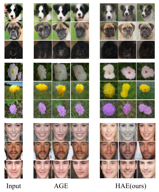
Qualitative Evaluation. We qualitatively compare our method with MatchingGAN Hong20Match, LoFGAN Gu21, DeltaGAN Hong22Delta and AGE Ding22. As shown in Fig. 19, HAE can generate images with diversity and fine-grained details. More importantly, the newly generated images have more semantic diversity than others. For instance, the shadow and skin color of the generated faces change with the light condition, and this effect looks more natural. We further conduct a user study by randomly selecting 60 (20 from each dataset) images with generated variants using AGE and HAE. 50 users from different backgrounds are asked to rate the results only based on diversity and quality external information. This is achieved by randomly shuffling the order of images pairwisely and inside any pair. HAE won by a ratio of over AGE (more details in supplementary).
Transferability. If we move latent codes at category-irrelevant levels, the target perturbation is transferable across all categories. We edit the images from three categories with the same editing direction, the output images are shown in Fig. 10. It demonstrates that HAE achieves a highly controllable and interpretable editing process.

| Method | Flowers | Animal Faces | VGG Faces | |||
| FID | LPIPS | FID | LPIPS | FID | LPIPS | |
| SAGE Ding23 | 43.52 | 0.4392 | 27.43 | 0.5448 | 34.97 | 0.3232 |
| HAE(Euc) | 54.62 | 0.4293 | 25.27 | 0.5129 | 38.46 | 0.5908 |
| HAE(Hyp) | 50.10 | 0.4739 | 26.33 | 0.5636 | 35.93 | 0.5919 |
4.5 Ablation Study
HAE in Euclidean. We re-trained HAE models in Euclidean space with the NLL loss to validate the performance gain in Table 1 is due to the hierarchical hyperbolic representation rather than the disentanglement caused by Eq. 7. The quantitative comparison is shown in Table 2. It shows that the hyperbolic space boosts the performance, especially for the LPIPS score, since the latent code is more disentangled in hyperbolic space Ge22. This finding is also supported by the UMAP visualization in Fig. 9. More details can be found in the supplementary material.


Hyperbolic Radius versus Truncation. StyleGAN Karras19 uses truncation trick Marchesi17; Brock19; Karras19; Karras20 in -space to achieve the balance between the image quality and diversity. The experiments in Karras19; Karras20 also show that the truncation level in -space control the level of abstraction of the generated images. We conduct the experiments in Section 3.4 using truncation to validate the gains of hyperbolic space. The results are illustrated in Fig. 11 and Fig. 12. As Fig. 11 shows, the category of the image changes along with the posture of the dog as the truncation gets smaller, while the category-relevant attributes do not change when the hyperbolic radius () is large. This can also be proved in Fig. 12. The category remains the same after adding perturbation when is large, while the truncation can not control semantic-level editing. This shows that Euclidean space can only capture scale-based hierarchy rather than the semantic hierarchy.
Downstream Task. We conduct data augmentation via HAE for image classification on Animal Faces Parkhi15. We randomly select 30, 35, and 35 images for each category as train, val, and test, respectively. Following Gu21, a ResNet-18 backbone is initialized from the seen categories. Then the model is fine-tuned on the unseen categories referred to as the baseline. 60 images are generated for each unseen category as data augmentation. The result is presented in Table 3. The diversity and quality of generated images are primarily controlled by the hyperbolic radii . As the radius becomes smaller, HAE generates images of higher diversity, but categories (referring to high-level attributes) also gradually change to others. achieves the best performance on the classification experiment. However, the performance drops when the radius is smaller than 4.5. This is because the semantic attributes change too much and thus mislead the classifier.
4.6 Limitations and Future Work
Although HAE achieves reliable hierarchical attribute editing in hyperbolic space for few-shot image generation, there are several limitations.
First, the boundary of category changing is hard to be quantified since the hierarchical levels are continuous in the hyperbolic space. Users need to find a “safe” boundary by trying different radii and step sizes of perturbation before generating new images. However, from another perspective, this continuity of hierarchy provides flexibility for users to set different boundaries for different downstream tasks as they need.
Second, the performance of HAE is limited by the pretrained styleGAN and the inversion method. If the input image can not be well embedded, the editing will also fail. This problem can be solved by changing more powerful backbones, e.g., ViT Dosovitskiy21, in future work.
Finally, we use supervised learning to get the hierarchical embedding in hyperbolic space. However, the number of images in existing datasets with labels for generation tasks is relatively small, which makes the embeddings in the hyperbolic space not evenly distributed. The solution to this problem is simple, use unsupervised learning with large-scale high-quality datasets.
| Hyperbolic Radius | Accuracy | FID() | LPIPS() |
|---|---|---|---|
| baseline | 58.67 | - | - |
| 6.0 | 60.10 | 46.89 | 0.4520 |
| 5.5 | 59.52 | 48.68 | 0.4651 |
| 5.0 | 59.05 | 52.08 | 0.4823 |
| 4.5 | 59.14 | 60.87 | 0.5174 |
| 4.0 | 58.57 | 65.83 | 0.5386 |
| 3.5 | 56.86 | 68.44 | 0.6034 |
| 3.0 | 54.14 | 69.40 | 0.6316 |
5 Conclusion
In this work, we propose a simple yet effective method HAE to edit hierarchical attributes in hyperbolic space. After learning the semantic hierarchy from images, our model is able to edit continuous semantic hierarchical features of images for flexible few-shot image generation in the hyperbolic space. Experiments demonstrate that HAE is capable of achieving not only stable few-shot image generation with state-of-the-art quality and diversity but a controllable and interpretable editing process. Future work includes the combination of HAE and large pretrained models and applications to more downstream tasks.
Acknowledgement. This work was supported in part by the National Key R&D Program of China under Grant 2018AAA0102000, in part by National Natural Science Foundation of China: 62022083 and 62236008.
References
- (1) Antreas Antoniou, Amos Storkey, and Harrison Edwards. Data augmentation generative adversarial networks. arXiv preprint arXiv:1711.04340, 2017.
- (2) Sergey Bartunov and Dmitry P. Vetrov. Few-shot generative modelling with generative matching networks. In AISTATS, 2018.
- (3) Silvère Bonnabel. Stochastic gradient descent on riemannian manifolds. IEEE Transactions on Automatic Control, 58(9):2217–2229, 2013.
- (4) Andrew Brock, Jeff Donahue, and Karen Simonyan. Large scale gan training for high fidelity natural image synthesis. In ICLR, 2019.
- (5) Gary Bécigneul and Octavian-Eugen Ganea. Riemannian adaptive optimization methods. In ICLR, 2019.
- (6) James W Cannon, William J Floyd, Richard Kenyon, and Walter R Parry. Hyperbolic geometry. Flavors of geometry, 31:59–115, 1997.
- (7) Ines Chami, Rex Ying, Christopher Ré, and Jure Leskovec. Hyperbolic graph convolutional neural networks. In NeurIPS, page 4868–4879, 2019.
- (8) Anton Cherepkov, Andrey Voynov, and Artem Babenko. Navigating the gan parameter space for semantic image editing. In CVPR, pages 3670–3679, 2021.
- (9) Jaewoong Choi, Junho Lee, Changyeon Yoon, Jung Ho Park, Geonho Hwang, and Myungjoo Kang. Do not escape from the manifold: Discovering the local coordinates on the latent space of gans. In ICLR, 2022.
- (10) Louis Clouâtre and Marc Demers. Figr: Few-shot image generation with reptile. arXiv:1901.02199, 2019.
- (11) Jiali Cui, Ying Nian Wu, and Tian Han. Learning joint latent space ebm prior model for multi-layer generator. In CVPR, pages 3603–3612, 2023.
- (12) Emily Denton, Ben Hutchinson, Margaret Mitchell, and Timnit Gebru. Detecting bias with generative counterfactual face attribute augmentation. CoRR, abs/1906.06439, 2019.
- (13) Bhuwan Dhingra, Chris Shallue, Mohammad Norouzi, Andrew Dai, and George Dahl. Embedding text in hyperbolic spaces. arXiv preprint arXiv:1806.04313, 2018.
- (14) Guanqi Ding, Xinzhe Han, Shuhui Wang, Xin Jin, Dandan Tu, and Qingming Huang. Stable attribute group editing for reliable few-shot image generation. arXiv preprint arXiv:2302.00179, 2023.
- (15) Guanqi Ding, Xinzhe Han, Shuhui Wang, Shuzhe Wu, Xin Jin, Dandan Tu, and Qingming Huang. Attribute group editing for reliable few-shot image generation. In CVPR, pages 11184–11193, 2022.
- (16) Alexey Dosovitskiy, Lucas Beyer, Alexander Kolesnikov, Dirk Weissenborn, Xiaohua Zhai, Thomas Unterthiner, Mostafa Dehghani, Matthias Minderer, Georg Heigold, Sylvain Gelly, Jakob Uszkoreit, and Neil Houlsby. An image is worth 16x16 words: Transformers for image recognition at scale. In ICLR, 2021.
- (17) Kun Fu, Tengfei Zhang, Yue Zhang, Menglong Yan, Zhonghan Chang, Zhengyuan Zhang, and Xian Sun. Meta-ssd: Towards fast adaptation for few-shot object detection with meta-learning. IEEE Access, 7:77597–77606, 2019.
- (18) Octavian-Eugen Ganea, Gary Bécigneul, and Thomas Hofmann. Hyperbolic neural networks. In NeurIPS, pages 5345–5355, 2018.
- (19) Songwei Ge, Shlok Mishra, Simon Kornblith, Chun-Liang Li, and David Jacobs. Hyperbolic contrastive learning for visual representations beyond objects. In CVPR, 2023.
- (20) Lore Goetschalckx, Alex Andonian, Aude Oliva, and Phillip Isola. Ganalyze: Toward visual definitions of cognitive image properties. In CVPR, page 5744–5753, 2019.
- (21) Ian Goodfellow, Jean Pouget-Abadie, Mehdi Mirza, Bing Xu, David Warde-Farley, Sherjil Ozair, Aaron Courville, and Yoshua Bengio. Generative adversarial nets. In NeurIPS, 2014.
- (22) Michael Gromov. Hyperbolic groups. In Essays in group theory, 1987.
- (23) Zheng Gu, Wenbin Li, Jing Huo, Lei Wang, and Yang Gao. Lofgan: Fusing local representations for fewshot image generation. In ICCV, 2021.
- (24) Martin Heusel, Hubert Ramsauer, Thomas Unterthiner, Bernhard Nessler, and Sepp Hochreiter. Gans trained by a two time-scale update rule converge to a local nash equilibrium. In NeurIPS, 2017.
- (25) Jonathan Ho, Ajay Jain, and Pieter Abbeel. Denoising diffusion probabilistic models. In ICLR, 2020.
- (26) Yan Hong, Li Niu, Jianfu Zhang, Jing Liang, and Liqing Zhang. Deltagan: Towards diverse few-shot image generation with sample-specific delta. In CVPR, 2020.
- (27) Yan Hong, Li Niu, Jianfu Zhang, Jing Liang, and Liqing Zhang. Deltagan: Towards diverse few-shot image generation with sample-specific delta. In ECCV, 2022.
- (28) Yan Hong, Li Niu, Jianfu Zhang, and Liqing Zhang. Matchinggan: Matching-based few-shot image generation. In 2020 IEEE International Conference on Multimedia and Expo (ICME), pages 1–6, 2020.
- (29) Yan Hong, Li Niu, Jianfu Zhang, and Liqing Zhang. Few-shot image generation using discrete content representation. In Proceedings of the 30th ACM International Conference on Multimedia, MM ’22, page 2796–2804, New York, NY, USA, 2022. Association for Computing Machinery.
- (30) Yan Hong, Li Niu, Jianfu Zhang, Weijie Zhao, Chen Fu, and Liqing Zhang. F2gan: Fusing-and-filling gan for few-shot image generation. In Proceedings of the 28th ACM International Conference on Multimedia, MM ’20, page 2535–2543. Association for Computing Machinery, 2020.
- (31) Erik Härkönen, Aaron Hertzmann, Jaakko Lehtinen, and Sylvain Paris. Ganspace: Discovering interpretable gan controls. In NeurIPS, 2020.
- (32) Ali Jahanian, Lucy Chai, and Phillip Isola. On the” steerability” of generative adversarial networks. In ICLR, 2020.
- (33) Tero Karras, Samuli Laine, and Timo Aila. A style-based generator architecture for generative adversarial networks. In CVPR, pages 4217–4228, 2019.
- (34) Tero Karras, Samuli Laine, Miika Aittala, Janne Hellsten, Jaakko Lehtinen, and Timo Aila. Analyzing and improving the image quality of stylegan. In CVPR, pages 8107–8116, 2020.
- (35) Valentin Khrulkov, Leyla Mirvakhabova, Evgeniya Ustinova, Ivan Oseledets, and Victor Lempitsky. Hyperbolic image embeddings. In CVPR, pages 6417–6427, 2020.
- (36) Diego Lazcano, Nicolás Fredes Franco, and Werner Creixell. Hgan: Hyperbolic generative adversarial network. IEEE Access, 9:96309–96320, 2021.
- (37) John M Lee. Riemannian manifolds: an introduction to curvature. Springer Science & Business Media, 176, 2006.
- (38) John M Lee. Introduction to Smooth Manifolds. Springer, 2013.
- (39) Weixin Liang, Zixuan Liu, and Can Liu. Dawson: A domain adaptive few shot generation framework. arXiv preprint arXiv:2001.00576, 2020.
- (40) Ming-Yu Liu, Xun Huang, Arun Mallya, Tero Karras, Timo Aila, Jaakko Lehtinen, and Jan Kautz. Few-shot unsueprvised image-to-image translation. In ICCV, 2019.
- (41) Yu-Ding Lu, Hsin-Ying Lee, Hung-Yu Tseng, and Ming-Hsuan Yang. Unsupervised discovery of disentangled manifolds in gans. arXiv preprint arXiv:2011.11842, 2020.
- (42) Marco Marchesi. Megapixel size image creation using generative adversarial networks. CoRR, abs/1706.00082, 2017.
- (43) Leland McInnes, John Healy, Nathaniel Saul, and Lukas Grossberger. Umap: Uniform manifold approximation and projection. The Journal of Open Source Software, 3(29):861, 2018.
- (44) Maximillian Nickel and Douwe Kiela. Generative visual manipulation on the natural image manifold. In ECCV, 2017.
- (45) Maximillian Nickel and Douwe Kiela. Learning continuous hierarchies in the lorentz model of hyperbolic geometry. In ICML, 2018.
- (46) Maria-Elena Nilsback and Andrew Zisserman. Automated flower classification over a large number of classes. In 2008 Sixth Indian Conference on Computer Vision, Graphics & Image Processing, pages 722–729, 2008.
- (47) Jiwoong Park, Junho Cho, Hyung Jin Chang, and Jin Young Choi. Unsupervised hyperbolic representation learning via message passing auto-encoders. In CVPR, pages 5512–5522, 2021.
- (48) Omkar M. Parkhi, Andrea Vedaldi, and Andrew Zisserman. Deep face recognition. In British Machine Vision Conference, 2015.
- (49) Elad Richardson, Yuval Alaluf, Or Patashnik, Yotam Nitzan, Yaniv Azar, Stav Shapiro, and Daniel Cohen-Or. Encoding in style: a stylegan encoder for image-to-image translation. In CVPR, pages 2287–2296, 2021.
- (50) Yujun Shen, Jinjin Gu, Xiaoou Tang, and Bolei Zhou. Interpreting the latent space of gans for semantic face editing. In CVPR, pages 9240–9249, 2020.
- (51) Yujun Shen and Bolei Zhou. Closed-form factorization of latent semantics in gans. In CVPR, pages 1532–1540, 2021.
- (52) Jiaming Song, Chenlin Meng, and Stefano Ermon. Denoising diffusion implicit models. In ICLR, 2021.
- (53) Nurit Spingarn-Eliezer, Ron Banner, and Tomer Michaeli. Gan ”steerability” without optimization. In ICLR, 2021.
- (54) Flood Sung, Yongxin Yang, Li Zhang, Tao Xiang, Philip H.S. Torr, and Timothy M. Hospedales. Learning to compare: Relation network for few-shot learning. In CVPR, pages 1199–1208, 2018.
- (55) Dídac Surís, Ruoshi Liu, and Carl Vondrick. Learning the predictability of the future. In CVPR, pages 12602–12612, 2021.
- (56) Alexandru Tifrea, Gary Bécigneul, and OctavianEugen Ganea. Poincaré glove: Hyperbolic word embeddings. In ICLR, 2019.
- (57) Oriol Vinyals, Charles Blundell, Timothy Lillicrap, Koray Kavukcuoglu, and Daan Wierstra. Matching networks for one shot learning. In NeurIPS, 2016.
- (58) Andrey Voynov and Artem Babenko. Unsupervised discovery of interpretable directions in the gan latent space. In ICML, pages 9786–9796, 2020.
- (59) Richard Zhang, Phillip Isola, Alexei A Efros, Eli Shechtman, and Oliver Wang. The unreasonable effectiveness of deep features as a perceptual metric. In CVPR, pages 586–595, 2018.
- (60) Jingyuan Zhu, Huimin Ma, Jiansheng Chen, and Jian Yuan. Few-shot image generation with diffusion models. arXiv preprint arXiv:2211.03264, 2022.
Supplementary Material
Overview
This appendix is organized as follows:
Appendix A provides the mathematical formulae used in hyperbolic neural networks. Sec 3.2 & Sec 3.3
Appendix B gives more implementation details of HAE. Sec 4.1
Appendix C shows the results of the ablation study of downstream tasks for Animal Faces Liu19Few, Flowers Nilsback08 and VGGFaces Parkhi15. Sec 4.3
Appendix D compares the embeddings of images in hyperbolic space and Euclidean space. Sec 4.4
Appendix E visualizes the interpolation on different radii in the Poincaré disk, along the geodesic, and on -space. Sec 4.3
Appendix F shows the images generated with different radii in the Poincaré disk. Sec 4.3
Appendix G compares the images generated by state-of-the-art few-shot image generation method, i.e. AGE Ding22 and our methods HAE. Sec 4.4
Appendix H gives more details of the user study we conducted. Sec 4.4
Appendix I gives more examples generated by HAE. Sec 4.4
Appendix A Hyperbolic Neural Networks
For hyperbolic spaces, since the metric is different from Euclidean space, the corresponding calculation operators also differ from Euclidean space. Recall that in Eq. (11), we have two operations: Möbius addition and Möbius scalar multiplication Khrulkov21, given fixed curvature .
For any given vectors , the Möbius addition is defined by:
| (13) |
where denotes the -norm of the vector, and denotes the Euclidean inner product of the vectors.
Similarly, the Möbius scalar multiplication of a scalar and a given vector is defined by:
| (14) |
We also would like to give explicit forms of the exponential map and the logarithmic map which are used in our model to achieve the translation between hyperbolic space and Euclidean space as mentioned in Sec 3.2.
The exponential map , that maps from the tangent spaces into the manifold, is given by
| (15) |
The logarithmic map is given by
| (16) |
Appendix B Implementation Details and Analysis
As mentioned in Sec 3.2, the output of : . The MLP encoder used in HAE, is split into three parts: , , and for encoding lower layer attributes, middle layer attributes, and higher layer attributes. The is a 5-layer MLP with a Leaky-ReLU (slope=0.2) activation function. The first three layers of are then fed into . The dimension of the output attribute is 128. Similar to , the is also an 5-layer MLP. 3-7 layers of is then fed into , the dimension of the output attribute is also 128. Different from and , is an 8-layer MLP. And we fed the last 12 layers attributes of into it. The dimension of the output attribute of is 256. Therefore, the final dimension of the Euclidean latent code is . While the MLP decoder is the reversed version of , taking as input and output .
During the training process, the constants defined in Eq. (10) are set as , , and changes dynamically based on the value of which guarantees that . Besides, we employ Adam optimizer with a learning rate of , and the batch size is set to 8.
In addition, as a remark, we choose the largest radius as in most of our experiments as in hyperbolic space since any vector asymptotically lying on the surface unit -sphere will have a hyperbolic length of approximately , which can be directly calculated by Eq. (2).
Finally, we want to show that HAE can be easily trained. The size of trainable parameters of HAE is around one hundred million which is small compared with other models with billions of parameters. It can be trained well within one day using a single NVIDIA TITAN RTX.
Appendix C Ablation Study of Downstream Task
Similar to the ablation study in Sec 4.3. We also conduct data augmentation via HAE for image classification on Animal Faces Liu19Few, Flowers Nilsback08, and VGGFaces Parkhi15. Due to the limited size of Flowers and VGGFaces datasets. We randomly select 10, 15 and 15 images for each category as train, val and test, respectively. Following Gu21; Ding22, a ResNet-18 backbone is initialized from the seen categories, then the model is fine-tuned on the unseen categories referred to as the baseline. 30 images are generated for each unseen category as data augmentation.
The result of Animal Faces is shown in Table 4. It shows that the accuracy of the classifier improves after using the AdamW optimizer. The experiment result essentially confirms the original result in Sec 4.3. The data augmentation improves the performance of the classifier when the hyperbolic radius is larger than 4. achieves the best performance on the classification experiment mainly because it achieves the best trade-off between the quality and diversity. However, the performance drops when the radius is smaller than 4. This is because the semantic attributes change too much and thus mislead the classifier.
The result of Flowers is presented in Table 5. Similar to the result of Animal Faces, the diversity and quality of generated images are largely controlled by the hyperbolic radii . As the radius becomes smaller, HAE generates images of higher diversity but categories also gradually change to others. achieves the best performance on the classification experiment.
However, Table 6 shows that all accuracy drops when we do data augmentation on VGGFaces dataset. We estimate that this is due to the low quality of inversion that harms the performance of the classifier. Besides, since we only select 10 images for each category for training, with the limited size of VGGFaces, it is easy to overfit. To evaluate our estimation, we further test the performance of the classifier trained by the original images and inversion images without any perturbation, denoted as inversion in Table 6. This result proves that our estimation is correct. The accuracy of the classifier trained by augmented images increases compared with the inversion, which shows that the augmentation still works and improves the generalization performance of our classifier. achieves the best performance on the classification experiment except the baseline.
It is also worth noticing that, the FID and LPIPS scores inTable 4, Table 5, and Table 6 are different from the scores we calculated in Sec 4.4. That is because we only use a very small subset of the data in this ablation study which can not represent the distribution of all images in the test dataset. Besides, the improvement of a classifier trained on augmented data is trivial, we believe this is due to the limitation of the encoding method,i.e. psp Richardson21 and generator,i.e. StyleGAN2 Karras20, which can not generate images with high enough quality.
| Hyperbolic Radius | Accuracy | FID() | LPIPS() |
|---|---|---|---|
| baseline | 67.34 | - | - |
| 6.0 | 68.22 | 46.89 | 0.4520 |
| 5.5 | 68.56 | 48.68 | 0.4651 |
| 5.0 | 69.33 | 52.08 | 0.4823 |
| 4.5 | 68.22 | 60.87 | 0.5174 |
| 4.0 | 67.67 | 65.83 | 0.5386 |
| 3.5 | 67.33 | 68.44 | 0.6034 |
| 3.0 | 66.89 | 69.40 | 0.6316 |
| Hyperbolic Radius | Accuracy | FID() | LPIPS() |
|---|---|---|---|
| baseline | 71.76 | - | - |
| 6.0 | 79.21 | 94.35 | 0.4640 |
| 5.5 | 77.25 | 98.09 | 0.4871 |
| 5.0 | 75.29 | 97.81 | 0.5110 |
| 4.5 | 78.82 | 97.53 | 0.5330 |
| 4.0 | 75.29 | 97.58 | 0.5499 |
| 3.5 | 73.33 | 101.52 | 0.6152 |
| 3.0 | 72.55 | 105.05 | 0.6439 |
| Hyperbolic Radius | Accuracy | FID() | LPIPS() |
| baseline | 77.99 | - | - |
| inversion | 69.53 | 25.46 | 0.2325 |
| 6.0 | 71.98 | 26.19 | 0.2702 |
| 5.5 | 72.53 | 26.46 | 0.2887 |
| 5.0 | 72.45 | 26.83 | 0.3080 |
| 4.5 | 72.32 | 26.92 | 0.3258 |
| 4.0 | 72.96 | 27.02 | 0.3405 |
| 3.5 | 74.05 | 26.35 | 0.4044 |
| 3.0 | 74.44 | 25.90 | 0.4411 |
Appendix D Comparison with Euclidean space
In this section, we mainly compare hyperbolic space with Euclidean space by UMAP visualization mcinnes2018umap-software, which is an extension of our analysis in Sec 4.4. Following the UMAP visualization on hyperbolic space for the Animal Faces Parkhi15 dataset, we first show the UMAP visualization of the embeddings of images in -space, where each embedding is of -dimension and therefore we resize them for UMAP calculation. The results for Euclidean UMAP of Animal Faces dataset are shown in Fig. 13. We observe that although the transition across different categories is smooth, there are no obvious clusters in the plot even for some significantly different species (e.g., polar bears and foxes).

We further carry on the experiments on the other two datasets. For Flowers Nilsback08 dataset, we use all images in the test dataset to generate the embeddings for both spaces, where there are 101 classes in total. The number of images in each class varies due to the original setting of the dataset. The results of the Flowers dataset are shown in Fig. 15, where clusters are more obvious in hyperbolic space and the similarity between classes is also well-reflected.
For the VGGFaces dataset Parkhi15, the results are shown in Fig. 16. Similarly, the clusters are better represented in hyperbolic settings. We observe that in hyperbolic space, images with similar low-level attributes (e.g., wearing black frame glasses, having mutton chops beard) are clustered. We need to pay attention to the small clusters in both plots where images are represented with tall rectangles (in the plot). These images do not share semantic attributes but are clustered together, which can be the influence of heavy watermarks on the images. This also encourages us to train the model with high-quality datasets for better GAN inversions.
Appendix E Interpolation Visualization
In this section, we offer a more detailed comparison of different radii and latent spaces. The results are shown in Fig. 17, where refers to the ratio of the whole geodesic described in Eq. (11) starting from image A to image B, e.g., when , the interpolation is exactly the hyperbolic mean of these two images. We observe that in -space, both high-level attributes and low-level attributes changed together while in hyperbolic space, we can achieve more detailed editing on low-level attributes while keeping high-level attributes unchanged, while the radius can control the degree of change more precisely. When the hyperbolic radius is large, the category of the given image remains the same before reaching the middle point of the curve. This property allows us to generate diverse images of the given image without changing its category-relevant attributes. As the hyperbolic radius becomes smaller, the higher-level attributes gradually change in the early stage of the interpolation. The interpolation visualization on geodesic shows that the image gradually changes from fine-grained to abstract to fine-grained. These results also explain our method of adding details by rescaling after taking the geodesic which will lead to a relatively abstract average.
Appendix F Images Generated with Different Radii
In this section, we give more examples of images generated by HAE with different radii in the Poincaré disk. As Fig. 18 shows, the high-level attributes, a.k.a. category-relevant attributes do not change when the radius is large which allows us to generate diverse images without changing the category. However, the images generated by HAE become more abstract and semantically diverse when the hyperbolic radius becomes smaller. The images gradually lose fine-grained details and change higher-level attributes as they move closer to the center of the Poincaré disk. For the few-shot image generation task, large radii work well since we want to change the category-irrelevant attributes of a given image. Nevertheless, our method HAE is not only capable of few-shot image generation but has great potential for other downstream tasks. For instance, HAE is able to generate a bunch of images of felines given an image of a cat. This can be done by rescaling the latent code to a relatively small radius in the hyperbolic space. Then we can add random perturbation to get the average code of multiple categories of felines. Finally, diverse images with fine-grained details of felines can be generated by moving those average codes to their children with larger radii.
Appendix G Comparison with State-of-the-art Few-shot Image Generation Method
We also provide a comparison of images generated by the state-of-the-art method, i.e. AGE Ding22 and our methods on three datasets. As Fig. 19 shows, our method is able to generate images with more semantic diversity. For instance, for dogs, HAE generates images with different light conditions and angles compared with images generated by AGE. Furthermore, for the woman in the third row from the bottom, HAE can change the image from a colored photo to a monochrome photo without changing her identity. However, our method also slightly changes some attributes compared with the original images, e.g., the hair color of dogs and the petal color of flowers. This is because the color varies within the category in these datasets which can indicate color is a category-irrelevant attribute for those categories. Therefore, our method does not change the category-relevant attributes but has more semantic diversity. Besides, images generated by HAE look more natural compared with images generated by AGE. Most importantly, AGE requires datasets with labels to learn the feature code book. However, the hierarchical representation in HAE can be learned using unsupervised or self-supervised learning if we have enough computing resources. Therefore, our work has great potential and can be applied to many other downstream tasks in future work.

Appendix H User Study
As mentioned, we conducted an extensive user study with a fully randomized survey. Results are shown in the main text. Specifically, we compared AGE and HAE in the following protocol:
- 1.
We randomly chose 20 images per dataset, and for each image, we then generated 3 variants using AGE and HAE, respectively. Overall, there were 60 original images and 180 generated variants in total.
- 2.
For each sample of each model, we grouped the 3 generated variants together, denoted as an image block. We then shuffled the following orders in the dataset: 1) order of images, 2) order of each block, 3) order of images in the block, an illustration is shown in Fig. 14.
- 3.
We gathered 50 volunteers from various backgrounds who were asked to choose one image block for one sampled image based on their evaluation of image diversity and quality subjectively. The results are then re-arranged.
The result breakdowns are shown as follows: Animal Faces: 658/1000; Flowers: 523/1000; VGGFaces: 562/1000. We also provide more examples used in the user study in Fig. 20.
Appendix I Additional Examples Generated by HAE
We provide more samples generated by HAE in Fig. 21, Fig. 22, and Fig. 23. The radius we choose is 6.2126 and the length of perturbation is 8.