Asymptotically Normal Estimation of Network Curvature

The use of distance matrices for data analysis is prevalent across numerous fields. Originating from applications in psychometrics, multidimensional scaling (MDS) (Torgerson 1952) pioneered the use of distance-based methods and has been explored in various domains, including the analysis of protein shapes (Havel and Wüthrich 1985), image classification Tenenbaum et al. 2000, and natural language processing Kusner et al. 2015. Notably, Hoff et al. 2002 introduced this idea in a model of social network formation, which has since been expanded in numerous ways, such as model-based clustering Handcock et al. 2007, multi-view networks Salter-Townshend and McCormick 2017, and dynamic networks Kim et al. 2018. Some models use mixtures of a block structure to model only at the individual level within a cluster of the network (Fosdick et al. 2016; Lok et al. 2021). Latent distance models have been applied to problems like modeling social influence (Sweet and Adhikari 2020), social media relationships of politicians (Lok et al. 2021), and neuron connectivity (Aliverti and Durante 2019), among others.

We focus on the properties of the geometric space underlying a latent distance model, particularly the notion of curvature. The sectional curvature of a latent space is broadly defined as the deviation from a flat (Euclidean) space via the growth of the circumference of small circles as a function of their radius. An important class of manifolds are those that are simply connected and have constant curvature. A classical result from Killing 1891 characterizes these as the spherical (positive curvature), Euclidean (0 or flat curvature), and hyperbolic (negative curvature) spaces. Though importantly, these do not represent the entire class of such manifolds.

Classically, the choice of the embedding space was at the discretion of the analyst. Notably, latent spherical and Euclidean spaces were used in Hoff et al. 2002. However, other metric spaces, particularly spherical and hyperbolic spaces, have been found to better represent many network data types Smith et al. 2017. The authors also provide a simulation-based approach to compare the eigenspectrum of the graph Laplacian to models under spherical, hyperbolic, and Euclidean geometry. They show how the latent embedding space influences observed properties of the network, notably the degree distribution and clustering of the network, which can influence the behavior of network contagion processes (i.e., SIR models) (Volz et al. 2011).

Our work bears the closest resemblance to that of Lubold et al. 2023, which discusses hypothesis testing of the latent space among a class of models and the estimation of the related distance matrix. Our work is distinct in several ways. Firstly, our method of estimating the curvature of the latent space is novel and useful for deriving interpretable asymptotic results. This is due to the fact that our method allows for an estimating equation approach to identifying curvature, which leads to desirable properties. Importantly, their approach tests whether the geometry can be embedded globally in each of the canonical spaces, whereas we provide a local approach derived from triangle distances. Furthermore, we also provide an improved latent distance estimator which allows for the construction of an asymptotically normal distance matrix, based on cliques (fully connected subgraphs) in a network. Our approach for curvature estimation is modular and can be applied to general distance matrices. Consequently, we illustrate how to test for constant curvature within an embedding space.

An alternative definition of graph curvature worth discussing includes the Ollivier-Ricci curvature (Ollivier 2007) and extensions such as Haantjes-Ricci curvature (Saucan et al. 2020) and Forman-Ricci curvature (Leal et al. 2018). These definitions of curvature are derived from metrics arising from graph distances (i.e., integer-valued shortest path distances) rather than distances on a smooth latent space. As such, it is not apparent what these estimates will converge to (or if they converge at all) when a network is studied as a random object, with the exception of van der Hoorn et al. 2020, who study a problem where connections are governed by a small radius on a latent space. The authors study the convergence of a modified Ollivier-Ricci curvature to the Ricci curvature of the underlying space in random geometric graphs under the limit of the connection radius shrinking to $0$. However, these discrete curvatures have also been applied to various settings, such as financial network instability (Sandhu et al. 2016; Samal et al. 2021), network sampling (Barkanass et al. 2022), cancer detection in gene regulatory networks (Sandhu et al. 2015), functional neuroscience (Farooq et al. 2019), and community detection (Sia et al. 2019; Ni et al. 2019).

We begin by defining the geometric environment. We assume points lie on a Riemannian manifold $\mathcal{M}^{p}$ of dimension $p$, equipped with a corresponding metric tensor $g$. The metric tensor can be used to define the sectional curvature of the manifold at a point $q\in\mathcal{M}^{p}$. For our purposes, we assume that this manifold is connected and that the curvature is both upper and lower bounded. In our problem, we exclusively work with distances and thus consider the metric space induced by the Riemannian manifold $\mathfrak{M}=(\mathcal{M}^{p},d)$. We include the related definitions of the metric tensor and the distance on the manifold in the appendix in Section D.

We further assume the manifold is a member of the class of simply connected Riemannian manifolds with constant sectional curvature $(\kappa)$. This assumption is consistent with work on the latent distance model in social networks (Hoff et al. 2002). These include the classical Euclidean $\mathbb{E}^{p}$ $(\kappa=0)$, spherical $\mathbb{S}^{p}(\kappa)$ $(\kappa>0)$, and, more recently, hyperbolic space $\mathbb{H}^{p}(\kappa)$ $(\kappa<0)$. The celebrated Killing-Hopf theorem states that these are the only manifolds of this type (Killing 1891; Hopf 1926). Therefore, we refer to these manifolds spaces as the canonical manifolds, and we introduce common representations of these manifolds later in this subsection.

To identify the curvature, we rely on a simple geometric insight, relating the side lengths of a triangle and the length of the triangle’s median; the line segment connecting a vertex to the midpoint of the opposite side.

In general, we require the manifold to satisfy two properties.

• •

  (A1) (Algebraic Midpoint Property) $\mathfrak{M}$ satisfies the algebraic midpoint property. For any $x,y\in\mathcal{M}^{p}$, there exists a point $z$ such that $d_{\mathcal{M}^{p}}(z,x)=d_{\mathcal{M}^{p}}(z,y)=\frac{1}{2}d_{\mathcal{M}^{p}}(x,y)$.

• •

  (A2) (Locally Euclidean) For all $q\in\mathcal{M}^{p}$, there exists some $\delta>0$ and some functions $c_{p},C_{p}$ such that for all $\epsilon\leq\delta$:

  $$c_{p}(\epsilon)\leq\frac{\text{Vol}(B_{\mathcal{M}^{p}}(\epsilon,q))}{\text{Vol}(B_{\mathbb{E}^{p}}(\epsilon,0))}\leq C_{p}(\epsilon)\text{ and }\lim_{\epsilon\to 0}\frac{\text{Vol}(B_{\mathcal{M}^{p}}(\epsilon,q))}{\text{Vol}(B_{\mathbb{E}^{p}}(\epsilon,0))}=1.$$

Here, $B_{\mathcal{M}^{p}}(\epsilon,q)$ is the $\epsilon$-ball on $\mathcal{M}^{p}$ centered at a point $q$, which we abbreviate to $B(\epsilon,q)$, and $B_{\mathbb{E}^{p}}(\epsilon,0)$ is the $\epsilon$-ball in Euclidean space. These conditions will hold under our mild assumptions on the manifold. See Section E in the supplementary materials for details. Next, we consider an explicit set of representations of the canonical manifold.

Canonical Manifolds.

Each of the canonical manifolds can be represented using a set of positions with real-valued vectors and a corresponding distance function, allowing for closed-form computation of the distances. We include definitions for Euclidean, spherical, and hyperbolic spaces for completeness. We emphasize the difference between the intrinsic and extrinsic geometry here. Though each of these canonical manifolds is embedded in $\mathbb{R}^{p}$, only the Euclidean space uses the standard $2$-norm to construct the distances. The curved canonical manifolds $\mathbb{S}^{p}$ and $\mathbb{H}^{p}(\kappa)$ can be embedded in $\mathbb{R}^{p+1}$ along with a properly defined metric. In the spherical example, we compute the length according to the path length on the surface of the sphere, rather than the Euclidean distance through the sphere. We next highlight each of these models.

The Euclidean manifold: $\mathbb{E}^{p}$ can be described using a set of points in $\mathbb{R}^{p}$ with the standard $2$-norm.

The spherical manifold: $\mathbb{S}^{p}$ with curvature $\kappa>0$ is equivalent to the sphere of radius $r=\frac{1}{\kappa^{2}}$. We express this using a set of coordinates $x\in\mathbb{R}^{p+1}$, such that $\sum_{k=0}^{p}x_{k}^{2}=1$. The distance on the sphere can be computed using the quadratic form $B_{\mathbb{S}^{p}}$ defined below:

The hyperbolic manifold: $\mathbb{H}^{p}$ with curvature $\kappa<0$ can be constructed using the hyperboloid model (Minkowski model), which corresponds to a set of points $x\in\mathbb{R}^{p+1}$, such that $x_{0}^{2}-\sum_{k=1}^{p}x_{k}^{2}=1,x_{0}>0$. An analogous quadratic form $B_{\mathbb{H}^{p}}$ exists for the hyperbolic embedding and can be used to compute the distances:

A number of methods exist to verify whether a particular set of distances can be embedded in a space of constant curvature, typically based on the zeros of eigenvalues of a transformation of the distance matrix. These include methods by Schoenberg 1935 and Begelfor and Werman 2005, as well as Cayley-Menger determinants (Blumenthal and Gillam 1943). Lubold et al. 2023 previously used such a criterion to identify whether a set of distances could be globally embedded in a particular curvature space. In this work, we take a different approach where we identify curvature based on a minimal set of points. We also estimate a specific curvature, rather than performing a test on the sign of the curvature, as presented by Lubold et al. 2023.

We rely on a simple geometric observation. Consider a set of three points that form a triangle and the length of the median. This length reveals the sectional curvature of the manifold, where a smaller distance corresponds to a more negatively curved space and a larger distance corresponds to a more positively curved space. This is visualized in Figure 1 for Euclidean, spherical, and hyperbolic triangles.

This use of midpoints helps to identify the curvature uniquely, when it may not be identified in other situations. For example, consider $4$ points placed equidistant from each other. This set of distances can be either represented in $\mathbb{E}^{3}$ as the tetrahedron, or using equidistant points on the sphere $\mathbb{S}^{2}(\kappa)$ for $\kappa>0$, making it impossible to identify the curvature of the space from this collection of distances alone.

We instead take a more direct approach to eliciting curvature by leveraging distances in a triangle and the triangle median (which, recall, is the distance from one vertex to the midpoint of the other two and distinct from the statistical median). This allows us to identify curvature with only four points in total. We now formalize this intuition. For any three points $x,y,z$ which lie in an unknown canonical manifold of dimension $p\geq 2$ with constant sectional curvature $\kappa$, $(x,y,z)$ can be isometrically embedded in a submanifold of dimension $2$. We illustrate this through the use of submanifolds that contain their geodesics, the paths on a manifold that minimize the path length between two points, and thus define a distance. Simply stated, even if the manifold’s dimension $p>2$, the curvature can be identified through the totally geodesic submanifold containing the triangle.

Some simple examples include the Euclidean plane, within the three-dimensional Euclidean space ($\mathbb{E}^{2}$ is a totally geodesic submanifold of $\mathbb{E}^{3}$). However, this is not always the case; consider the two-dimensional sphere $\mathbb{S}^{2}(\kappa)$, which also resides within three-dimensional Euclidean space but does not contain all of its geodesics, as these geodesics in $\mathbb{E}^{3}$ pass through the center of the sphere. This distinction highlights the differences between intrinsic and extrinsic notions of distance, as our object of study is the former. We will use the fact that a totally geodesic submanifold contains all points along the geodesic, including the midpoint.

The intuition behind this lemma is that, regardless of the ambient dimension of the latent manifold $p$, we can determine the curvature from a two-dimensional submanifold. This submanifold is constructed from the geodesics of a given triangle. As we will see in Theorem 3, the side lengths and the length of the triangle’s median are sufficient to identify the curvature of the manifold. The proof is straightforward and in Section A.1. The main implication here is that the totally geodesic submanifold allows us to look at the distances in a subspace of dimension $2$ which will be useful in the following theorem for identification. The three points $x,y,z$ will fall into one of these sub-manifolds, as well as $m$ which lies on the geodesic between $y$ and $z$. Since geodesics determine the distance, and geodesics on the submanifold are the same as geodesics on the manifold.

We now use this fact to derive an equation which will relate the curvature $\kappa$ to the set of distances between the points $(x,y,z,m)$, which we denote $\boldsymbol{d}^{\mathchoice{{\displaystyle\displaystyle 3\vtop{\halign{#\cr\hfil\hbox{\vrule width=5.54767pt,height=4.8611pt,depth=-2.77383pt}\hfil\cr\hbox{$\displaystyle\bigtriangleup$}\crcr}}}}{{\textstyle\displaystyle 3\vtop{\halign{#\cr\hfil\hbox{\vrule width=5.54767pt,height=4.8611pt,depth=-2.77383pt}\hfil\cr\hbox{$\textstyle\bigtriangleup$}\crcr}}}}{{\scriptstyle\displaystyle 3\vtop{\halign{#\cr\hfil\hbox{\vrule width=5.54767pt,height=3.40277pt,depth=-2.77383pt}\hfil\cr\hbox{$\scriptstyle\bigtriangleup$}\crcr}}}}{{\scriptscriptstyle\displaystyle 3\vtop{\halign{#\cr\hfil\hbox{\vrule width=5.54767pt,height=2.43054pt,depth=-2.77383pt}\hfil\cr\hbox{$\scriptscriptstyle\bigtriangleup$}\crcr}}}}}=(d_{xy},d_{xz},d_{yz},d_{xm})$.

The proof first leverages the fact that by Lemma 2, we can construct a submanifold of dimension 2 that contains the midpoint of points on a triangle. We then use this to derive an equation that relates the side lengths of the triangle, the triangle median length, and the curvature of the space. For cases when $\kappa<0$, we take the real part of equation (1), which is equivalent to replacing the trigonometric functions with their hyperbolic analogues. Though this does require that $p\geq 2$, this covers most manifolds of interest. The proof is found in the supplementary materials in Section A.2. It will also be convenient to express the length of the triangle median $d_{xm}(\kappa;\boldsymbol{d}^{\triangle}(x,y,z))$ as a function of the curvature $\kappa$ and a set of triangle side lengths $\boldsymbol{d}^{\triangle}(x,y,z)$.

We remark on the a similar criterion used by Gu et al. 2018 for identifying the number of components of positive and negative curvature in a product-space embedding.  Gu et al. 2018 derive the parameter $\theta_{T}$ from Toponogov’s theorem (which can be found in the appendix Theorem 12) and its sign can be used to identify the sign of the curvature of the manifold. In fact, it is straightforward to show $\lim_{\kappa\to 0}g(\kappa,\boldsymbol{d}^{\mathchoice{{\displaystyle\displaystyle 3\vtop{\halign{#\cr\hfil\hbox{\vrule width=5.54767pt,height=4.8611pt,depth=-2.77383pt}\hfil\cr\hbox{$\displaystyle\bigtriangleup$}\crcr}}}}{{\textstyle\displaystyle 3\vtop{\halign{#\cr\hfil\hbox{\vrule width=5.54767pt,height=4.8611pt,depth=-2.77383pt}\hfil\cr\hbox{$\textstyle\bigtriangleup$}\crcr}}}}{{\scriptstyle\displaystyle 3\vtop{\halign{#\cr\hfil\hbox{\vrule width=5.54767pt,height=3.40277pt,depth=-2.77383pt}\hfil\cr\hbox{$\scriptstyle\bigtriangleup$}\crcr}}}}{{\scriptscriptstyle\displaystyle 3\vtop{\halign{#\cr\hfil\hbox{\vrule width=5.54767pt,height=2.43054pt,depth=-2.77383pt}\hfil\cr\hbox{$\scriptscriptstyle\bigtriangleup$}\crcr}}}}})=\theta_{T}(\boldsymbol{d}^{\mathchoice{{\displaystyle\displaystyle 3\vtop{\halign{#\cr\hfil\hbox{\vrule width=5.54767pt,height=4.8611pt,depth=-2.77383pt}\hfil\cr\hbox{$\displaystyle\bigtriangleup$}\crcr}}}}{{\textstyle\displaystyle 3\vtop{\halign{#\cr\hfil\hbox{\vrule width=5.54767pt,height=4.8611pt,depth=-2.77383pt}\hfil\cr\hbox{$\textstyle\bigtriangleup$}\crcr}}}}{{\scriptstyle\displaystyle 3\vtop{\halign{#\cr\hfil\hbox{\vrule width=5.54767pt,height=3.40277pt,depth=-2.77383pt}\hfil\cr\hbox{$\scriptstyle\bigtriangleup$}\crcr}}}}{{\scriptscriptstyle\displaystyle 3\vtop{\halign{#\cr\hfil\hbox{\vrule width=5.54767pt,height=2.43054pt,depth=-2.77383pt}\hfil\cr\hbox{$\scriptscriptstyle\bigtriangleup$}\crcr}}}}})$. If the sectional curvature of $\mathcal{M}^{p}$ is positive, then $\theta_{T}(\boldsymbol{d}^{\mathchoice{{\displaystyle\displaystyle 3\vtop{\halign{#\cr\hfil\hbox{\vrule width=5.54767pt,height=4.8611pt,depth=-2.77383pt}\hfil\cr\hbox{$\displaystyle\bigtriangleup$}\crcr}}}}{{\textstyle\displaystyle 3\vtop{\halign{#\cr\hfil\hbox{\vrule width=5.54767pt,height=4.8611pt,depth=-2.77383pt}\hfil\cr\hbox{$\textstyle\bigtriangleup$}\crcr}}}}{{\scriptstyle\displaystyle 3\vtop{\halign{#\cr\hfil\hbox{\vrule width=5.54767pt,height=3.40277pt,depth=-2.77383pt}\hfil\cr\hbox{$\scriptstyle\bigtriangleup$}\crcr}}}}{{\scriptscriptstyle\displaystyle 3\vtop{\halign{#\cr\hfil\hbox{\vrule width=5.54767pt,height=2.43054pt,depth=-2.77383pt}\hfil\cr\hbox{$\scriptscriptstyle\bigtriangleup$}\crcr}}}}})>0$, and if the curvature is negative, $\theta_{T}(\boldsymbol{d}^{\mathchoice{{\displaystyle\displaystyle 3\vtop{\halign{#\cr\hfil\hbox{\vrule width=5.54767pt,height=4.8611pt,depth=-2.77383pt}\hfil\cr\hbox{$\displaystyle\bigtriangleup$}\crcr}}}}{{\textstyle\displaystyle 3\vtop{\halign{#\cr\hfil\hbox{\vrule width=5.54767pt,height=4.8611pt,depth=-2.77383pt}\hfil\cr\hbox{$\textstyle\bigtriangleup$}\crcr}}}}{{\scriptstyle\displaystyle 3\vtop{\halign{#\cr\hfil\hbox{\vrule width=5.54767pt,height=3.40277pt,depth=-2.77383pt}\hfil\cr\hbox{$\scriptstyle\bigtriangleup$}\crcr}}}}{{\scriptscriptstyle\displaystyle 3\vtop{\halign{#\cr\hfil\hbox{\vrule width=5.54767pt,height=2.43054pt,depth=-2.77383pt}\hfil\cr\hbox{$\scriptscriptstyle\bigtriangleup$}\crcr}}}}})<0$. In Euclidean space, $\theta_{T}(\boldsymbol{d}^{\mathchoice{{\displaystyle\displaystyle 3\vtop{\halign{#\cr\hfil\hbox{\vrule width=5.54767pt,height=4.8611pt,depth=-2.77383pt}\hfil\cr\hbox{$\displaystyle\bigtriangleup$}\crcr}}}}{{\textstyle\displaystyle 3\vtop{\halign{#\cr\hfil\hbox{\vrule width=5.54767pt,height=4.8611pt,depth=-2.77383pt}\hfil\cr\hbox{$\textstyle\bigtriangleup$}\crcr}}}}{{\scriptstyle\displaystyle 3\vtop{\halign{#\cr\hfil\hbox{\vrule width=5.54767pt,height=3.40277pt,depth=-2.77383pt}\hfil\cr\hbox{$\scriptstyle\bigtriangleup$}\crcr}}}}{{\scriptscriptstyle\displaystyle 3\vtop{\halign{#\cr\hfil\hbox{\vrule width=5.54767pt,height=2.43054pt,depth=-2.77383pt}\hfil\cr\hbox{$\scriptscriptstyle\bigtriangleup$}\crcr}}}}})=0$, and this reduces to the parallelogram law. Our method is distinct as it directly identifies the curvature using this same set of distances, rather than the sign of the curvature.

If the true manifold that generates the distances is non-constant, then the value $\kappa$ is the curvature of the 2-dimensional canonical manifold which can isometrically embed a set of triangle distances $\boldsymbol{d}^{\mathchoice{{\displaystyle\displaystyle 3\vtop{\halign{#\cr\hfil\hbox{\vrule width=5.54767pt,height=4.8611pt,depth=-2.77383pt}\hfil\cr\hbox{$\displaystyle\bigtriangleup$}\crcr}}}}{{\textstyle\displaystyle 3\vtop{\halign{#\cr\hfil\hbox{\vrule width=5.54767pt,height=4.8611pt,depth=-2.77383pt}\hfil\cr\hbox{$\textstyle\bigtriangleup$}\crcr}}}}{{\scriptstyle\displaystyle 3\vtop{\halign{#\cr\hfil\hbox{\vrule width=5.54767pt,height=3.40277pt,depth=-2.77383pt}\hfil\cr\hbox{$\scriptstyle\bigtriangleup$}\crcr}}}}{{\scriptscriptstyle\displaystyle 3\vtop{\halign{#\cr\hfil\hbox{\vrule width=5.54767pt,height=2.43054pt,depth=-2.77383pt}\hfil\cr\hbox{$\scriptscriptstyle\bigtriangleup$}\crcr}}}}}$.

Our method differs from those of Schoenberg 1935 and the Cayley-Menger determinants (Blumenthal and Gillam 1943) because it requires midpoint information, which theirs do not. Their methods do not uniquely identify curvature but only determine if a space of constant curvature can embed an given distance matrix. In the appendix, we illustrate the smoothness of this equation, which is also a desirable property for plug-in estimators (Section H.2).

In this subsection, we describe how to estimate the curvature from a noisy estimate of a set of distances using Theorem 3. We begin by introducing an estimator based on triangle distances and its median length. In practice, we are often given an estimate of a distance matrix between an arbitrary set of $K$ points $\boldsymbol{D}\in\mathbb{R}^{K\times K}$. In this setting, it is not guaranteed that there is a midpoint of two other points among the observed points in the distance matrix. We illustrate how one can bound the curvature in this setting. Lastly, we introduce a result that characterizes the formation of points arbitrarily close to the midpoint of other points.

We first consider an idealized scenario. In this setting, we suppose that we are given an estimate of the triangle distances $\boldsymbol{\widehat{d}}^{\mathchoice{{\displaystyle\displaystyle 3\vtop{\halign{#\cr\hfil\hbox{\vrule width=5.54767pt,height=4.8611pt,depth=-2.77383pt}\hfil\cr\hbox{$\displaystyle\bigtriangleup$}\crcr}}}}{{\textstyle\displaystyle 3\vtop{\halign{#\cr\hfil\hbox{\vrule width=5.54767pt,height=4.8611pt,depth=-2.77383pt}\hfil\cr\hbox{$\textstyle\bigtriangleup$}\crcr}}}}{{\scriptstyle\displaystyle 3\vtop{\halign{#\cr\hfil\hbox{\vrule width=5.54767pt,height=3.40277pt,depth=-2.77383pt}\hfil\cr\hbox{$\scriptstyle\bigtriangleup$}\crcr}}}}{{\scriptscriptstyle\displaystyle 3\vtop{\halign{#\cr\hfil\hbox{\vrule width=5.54767pt,height=2.43054pt,depth=-2.77383pt}\hfil\cr\hbox{$\scriptscriptstyle\bigtriangleup$}\crcr}}}}}$. We return to the problem of estimating distances in our model in Section 2.5. We can use such a set of noisy or estimated distances to estimate the curvature ($\widehat{\kappa}$) by solving for the value of $\kappa$ which is the solution to equation 2.

The advantage of this method is that the smoothness of $g$ allows for the derivation of explicit asymptotics for $\widehat{\kappa}$, which is not possible for the method used by Lubold et al. 2023. We present this result below in Theorem 4.

The proof is found in the supplementary materials in Section A.3 and is an application of the implicit function theorem together with the delta method. Assumption (B1) is mild as it only requires asymptotic normality of the distance estimator. Assumption (B2) is trivial since it simply requires that the true distances are not greater than the maximum allowable distances on the sphere of curvature $\kappa$. Assumption (B3) tends to hold unless the three points $x,y,z$ are collinear. For a more in-depth discussion of the non-decreasing property of the midpoint, see Lemma 11 in the appendix. In Section 2.5, we illustrate the asymptotic normality of a distance estimator based on cliques. We next discuss the bias associated when a set of pairwise distances are observed, where no point is necessarily a midpoint of another pair of points.

In general, rather than distances from a triangle median, we may only observe distances in the form of a distance matrix $\boldsymbol{D}\in\mathbb{R}^{K\times K}$. There might not be a midpoint between two other points within this set. In this case, given a triangle, we can use a point nearby to the midpoint as a surrogate midpoint $m^{\prime}$ taking the role of a midpoint between $y,z$.

We let $\kappa^{\prime}$ be the solution to equation (2) where $d_{xm^{\prime}}$ takes the place of $d_{xm}$. In this case, we can approximate the bias of the curvature estimate using a Taylor series expansion.

Therefore, the bias will scale approximately linearly as a function of $d_{mm^{\prime}}$ for small values of $d_{mm^{\prime}}$.

If four points are within a manifold of constant curvature $x,y,z,m^{\prime}\in\mathcal{M}^{p}(\kappa)$, then using the curvature value $\kappa$, one can compute the distance from the midpoint $m$ to $m^{\prime}$ by letting $m^{\prime}$ take the place in equation (1) and solving for $d_{mm^{\prime}}$. As such, we denote this $d_{mm^{\prime}}(\kappa):=d_{m^{\prime}m}(\kappa;\boldsymbol{d}^{\triangle}(y,z,m^{\prime}))$ as a function of the curvature. Using the triangle inequality, we can then upper and lower bound the curvature by replacing $d_{xm}$ with upper and lower bounds in equation (1) and solving the corresponding equations. We illustrate this in Theorem 5.

For a given $\kappa$, let $\boldsymbol{d^{\mathchoice{{\displaystyle\displaystyle 3\vtop{\halign{#\cr\hfil\hbox{\vrule width=5.44983pt,height=4.8611pt,depth=-2.72491pt}\hfil\cr\hbox{$\displaystyle\bigtriangleup$}\crcr}}}}{{\textstyle\displaystyle 3\vtop{\halign{#\cr\hfil\hbox{\vrule width=5.44983pt,height=4.8611pt,depth=-2.72491pt}\hfil\cr\hbox{$\textstyle\bigtriangleup$}\crcr}}}}{{\scriptstyle\displaystyle 3\vtop{\halign{#\cr\hfil\hbox{\vrule width=5.44983pt,height=3.40277pt,depth=-2.72491pt}\hfil\cr\hbox{$\scriptstyle\bigtriangleup$}\crcr}}}}{{\scriptscriptstyle\displaystyle 3\vtop{\halign{#\cr\hfil\hbox{\vrule width=5.44983pt,height=2.43054pt,depth=-2.72491pt}\hfil\cr\hbox{$\scriptscriptstyle\bigtriangleup$}\crcr}}}},+}}(\kappa)=(d_{xy},d_{xz},d_{yz},d_{xm^{\prime}}+d_{mm^{\prime}}(\kappa))$ and $\boldsymbol{d^{\mathchoice{{\displaystyle\displaystyle 3\vtop{\halign{#\cr\hfil\hbox{\vrule width=5.44983pt,height=4.8611pt,depth=-2.72491pt}\hfil\cr\hbox{$\displaystyle\bigtriangleup$}\crcr}}}}{{\textstyle\displaystyle 3\vtop{\halign{#\cr\hfil\hbox{\vrule width=5.44983pt,height=4.8611pt,depth=-2.72491pt}\hfil\cr\hbox{$\textstyle\bigtriangleup$}\crcr}}}}{{\scriptstyle\displaystyle 3\vtop{\halign{#\cr\hfil\hbox{\vrule width=5.44983pt,height=3.40277pt,depth=-2.72491pt}\hfil\cr\hbox{$\scriptstyle\bigtriangleup$}\crcr}}}}{{\scriptscriptstyle\displaystyle 3\vtop{\halign{#\cr\hfil\hbox{\vrule width=5.44983pt,height=2.43054pt,depth=-2.72491pt}\hfil\cr\hbox{$\scriptscriptstyle\bigtriangleup$}\crcr}}}},-}}(\kappa)=(d_{xy},d_{xz},d_{yz},d_{xm^{\prime}}-d_{mm^{\prime}}(\kappa))$.

When the surrogate midpoint and the true midpoint are the same, then $d_{mm^{\prime}}=0$ and the upper and lower bounds converge. Similar to the curvature estimate $\widehat{\kappa}$, given a noisy estimate of the distances, we can estimate the upper and lower bounds of the curvature. In Section 4, we leverage these bounds to develop a test of constant curvature. We next address the formation of surrogate midpoints arbitrarily close to the midpoints of other pairs of points.

We next provide an outline involving how fast we can expect surrogate midpoints to form. In order to do so, we first introduce a useful definition. A subset $A\subset\mathcal{M}^{p}$ is geodesically convex if the geodesic between any two points in $A$ is contained within $A$ itself. Here, convexity on a manifold will refer to geodesic convexity. In Theorem 6, we let $h_{m,3}(m_{1},m_{2})$ denote the joint density function of a pair of midpoints with a shared endpoint and $h_{m,4}(m_{1},m_{2})$ denote the joint density of two midpoints without a shared endpoint. These two densities will be functions of the unknown manifold $\mathcal{M}$ and the distribution of the positions $Z^{\prime}$, $G_{Z^{\prime}}$.

Our approach to demonstrating the above result draws on the work of Cai et al. 2013 and Brauchart et al. 2015, who discuss the convergence of the minimum distance between any two points sampled uniformly on a hypersphere. These authors show that $\min_{i,j}d(Z_{i},Z_{j})=\mathcal{O}_{P}(K^{-2/p})$, and they also derive an exact distribution for $\min_{i,j}d(Z_{i},Z_{j})$ under the assumption of uniformity on the sphere. They use a technique that recursively computes the probability that a point is at least a radius $\epsilon$ away from the previous $K$ points. In our approach, at each placement of a new point, there are $\binom{K}{2}$ midpoints instead of $K$ current points, leading to the faster rate we observe.

Assumption (C1) ensures the existence of geodesically convex regions for which midpoints can form. Assumption (C2) ensures that this region has the same dimension as the ambient space. Lastly, Assumption (C3) is relatively mild as long as we have a smooth manifold and a continuous density. The proof is detailed in Section A.5 of the supplementary materials and relies on a result regarding medians of arbitrarily correlated random variables, which may be of independent interest (Theorem 13).

When given an estimate of a distance matrix and to later apply our method, as in many statistical problems, we are concerned with the bias and variance of our estimator. The variance, in general, will be driven by the shape of the triangle used to estimate the curvature, while the bias will be driven by the closeness of the surrogate midpoint to the true midpoint of a triangle. We first visualize this phenomenon and then follow up by providing some practical strategies for constructing good estimators.

We can visualize the theoretical variance by using our asymptotic result in Theorem 4. In Figure 3, we plot the variance of the curvature estimate for a distance estimator with identity variance (i.e., $\boldsymbol{\widehat{d}}^{\mathchoice{{\displaystyle\displaystyle 3\vtop{\halign{#\cr\hfil\hbox{\vrule width=5.54767pt,height=4.8611pt,depth=-2.77383pt}\hfil\cr\hbox{$\displaystyle\bigtriangleup$}\crcr}}}}{{\textstyle\displaystyle 3\vtop{\halign{#\cr\hfil\hbox{\vrule width=5.54767pt,height=4.8611pt,depth=-2.77383pt}\hfil\cr\hbox{$\textstyle\bigtriangleup$}\crcr}}}}{{\scriptstyle\displaystyle 3\vtop{\halign{#\cr\hfil\hbox{\vrule width=5.54767pt,height=3.40277pt,depth=-2.77383pt}\hfil\cr\hbox{$\scriptstyle\bigtriangleup$}\crcr}}}}{{\scriptscriptstyle\displaystyle 3\vtop{\halign{#\cr\hfil\hbox{\vrule width=5.54767pt,height=2.43054pt,depth=-2.77383pt}\hfil\cr\hbox{$\scriptscriptstyle\bigtriangleup$}\crcr}}}}}\sim N(\boldsymbol{d}^{\mathchoice{{\displaystyle\displaystyle 3\vtop{\halign{#\cr\hfil\hbox{\vrule width=5.54767pt,height=4.8611pt,depth=-2.77383pt}\hfil\cr\hbox{$\displaystyle\bigtriangleup$}\crcr}}}}{{\textstyle\displaystyle 3\vtop{\halign{#\cr\hfil\hbox{\vrule width=5.54767pt,height=4.8611pt,depth=-2.77383pt}\hfil\cr\hbox{$\textstyle\bigtriangleup$}\crcr}}}}{{\scriptstyle\displaystyle 3\vtop{\halign{#\cr\hfil\hbox{\vrule width=5.54767pt,height=3.40277pt,depth=-2.77383pt}\hfil\cr\hbox{$\scriptstyle\bigtriangleup$}\crcr}}}}{{\scriptscriptstyle\displaystyle 3\vtop{\halign{#\cr\hfil\hbox{\vrule width=5.54767pt,height=2.43054pt,depth=-2.77383pt}\hfil\cr\hbox{$\scriptscriptstyle\bigtriangleup$}\crcr}}}}0},I_{4\times 4})$) for a variety of choices of $\kappa$. In this plot, we change the position of the vertex $x$ of the triangle (which we may also refer to as the reference point). The smallest variance reference points across all of these curvatures are the ones that form nearly equilateral triangles with the points $y,z$. Additionally, the variance of the estimator tends to be larger in a given reference location as the curvature $\kappa$ decreases. We plot all reference points $x$ within a ball of radius 2. Secondly, we illustrate, for an equilateral triangle, the bias of the estimate of the curvature when moving the location of the surrogate midpoint $m^{\prime}$. The spherical and hyperbolic spaces are shown using a projection where the distance to the center and relative angle are mapped onto Euclidean space.

We next illustrate some practical choices to minimize the bias and variance of a curvature estimate from a distance matrix $\boldsymbol{\widehat{D}}$.

Choosing the Best Midpoint. In practice, we would like to search over the space to find the best midpoint between two other points in the distance matrix. The midpoint between any two points $y,z$ is also known as the Fréchet mean, which is defined as follows:

In practice we search over the space of candidate entries of a distance matrix $D$ to find the best midpoint available. We also want to ensure that the points $y,z$ are not too close to each other since this tends to lead to a high variance estimator. A reasonable option is to normalize this quantity by $d_{yz}$. Given a true midpoint $m^{*}$, then $d_{ym^{*}}=d_{zm^{*}}=\frac{1}{2}d_{yz}$, then

We can also add a term $\frac{|d_{ym}-d_{zm}|}{d_{yz}}$ which aids in balancing the lengths of the distance to each point.

Therefore, to compute the best surrogate midpoint set, we solve the following problem:

In cases where we are interested in measuring the curvature across multiple surrogate midpoint sets, we remove this set of points and solve equation (6) for the remaining indices to construct a collection of surrogate midpoint set $\{(y^{(j)},z^{(j)},m^{(j)})\}_{j=1}^{J}$.

Selecting the Best Triangles. Given a surrogate midpoint set $(y,m^{\prime},z)$, we seek to find choices for the reference point $x$ which provide the lowest variance. A good rule of thumb is to search for triangles $x,y,z$ that are nearly equilateral.

We exploit this by considering a scaled version of the triangle inequality. Let $C_{\triangle}\in[1,2]$ be a constant that determines the flatness of the allowed triangles $x,y,z$. Then we select only the $x$ such that

If one believes that the curvature is constant across a surrogate midpoint set, we can estimate a single curvature by taking the median across the values of $x$. This tuning parameter allows us to pick the triangles closest to equilateral, which tend to give the best estimates of the curvature. Letting $C_{\triangle}=1$ allows for all triangles, no matter how flat they are, and $C_{\triangle}=2$ will only permit exact equilateral triangles. Setting $C_{\triangle}$ too large results in no triangles being found, and setting $C_{\triangle}$ too small will result in using triangles that are very flat, often suffering from high variance in the corresponding $\widehat{\kappa}$ estimates. In practice, we find that a value of $C_{\triangle}\in[1.05,1.7]$ is effective, and a good default choice is $1.3$.

From an estimated distance matrix $\boldsymbol{\widehat{D}}$, we let $\boldsymbol{X}_{\boldsymbol{\widehat{D}},C_{\triangle}}=\{x:\text{ eq}~\eqref{eq:triangle_tuning}\}$ denote the set of reference points used for curvature estimation. We let $\widehat{\kappa}_{x}=\kappa(\boldsymbol{\widehat{D}},\boldsymbol{\widehat{d}}^{\mathchoice{{\displaystyle\displaystyle 3\vtop{\halign{#\cr\hfil\hbox{\vrule width=5.54767pt,height=4.8611pt,depth=-2.77383pt}\hfil\cr\hbox{$\displaystyle\bigtriangleup$}\crcr}}}}{{\textstyle\displaystyle 3\vtop{\halign{#\cr\hfil\hbox{\vrule width=5.54767pt,height=4.8611pt,depth=-2.77383pt}\hfil\cr\hbox{$\textstyle\bigtriangleup$}\crcr}}}}{{\scriptstyle\displaystyle 3\vtop{\halign{#\cr\hfil\hbox{\vrule width=5.54767pt,height=3.40277pt,depth=-2.77383pt}\hfil\cr\hbox{$\scriptstyle\bigtriangleup$}\crcr}}}}{{\scriptscriptstyle\displaystyle 3\vtop{\halign{#\cr\hfil\hbox{\vrule width=5.54767pt,height=2.43054pt,depth=-2.77383pt}\hfil\cr\hbox{$\scriptscriptstyle\bigtriangleup$}\crcr}}}}}(x,y,z,m^{\prime}))$, where $\boldsymbol{\widehat{d}}^{\mathchoice{{\displaystyle\displaystyle 3\vtop{\halign{#\cr\hfil\hbox{\vrule width=5.54767pt,height=4.8611pt,depth=-2.77383pt}\hfil\cr\hbox{$\displaystyle\bigtriangleup$}\crcr}}}}{{\textstyle\displaystyle 3\vtop{\halign{#\cr\hfil\hbox{\vrule width=5.54767pt,height=4.8611pt,depth=-2.77383pt}\hfil\cr\hbox{$\textstyle\bigtriangleup$}\crcr}}}}{{\scriptstyle\displaystyle 3\vtop{\halign{#\cr\hfil\hbox{\vrule width=5.54767pt,height=3.40277pt,depth=-2.77383pt}\hfil\cr\hbox{$\scriptstyle\bigtriangleup$}\crcr}}}}{{\scriptscriptstyle\displaystyle 3\vtop{\halign{#\cr\hfil\hbox{\vrule width=5.54767pt,height=2.43054pt,depth=-2.77383pt}\hfil\cr\hbox{$\scriptscriptstyle\bigtriangleup$}\crcr}}}}}(x,y,z,m^{\prime})$ denotes the estimated distances of the triangle $(x,y,z)$ with surrogate midpoint $m^{\prime}$. Let $\widehat{\kappa}_{med}=\text{median}\{\widehat{\kappa}_{x}\}$. Given $\boldsymbol{X}$, we can construct the median estimator $\widehat{\kappa}_{med,\boldsymbol{X}}$ of the curvature in equation (8).

We now turn to estimating the distance matrix $\boldsymbol{\widehat{D}}$ in a latent distance model.

We consider the random undirected network corresponding to a graph $G=(V,E)$ where $|V|=n$, with adjacency matrix $A\in\{0,1\}^{n\times n}$ such that $A_{ij}=1$ iff $(i,j)\in E$. We motivate our method through the latent distance model of network formation Hoff et al. 2002. This is one specific choice of distance model that we will focus on, but it is not the only option. In this model, locations $Z_{i},Z_{j}$ are most generally equipped to some metric $d(\cdot,\cdot)$, forming a metric space, $\mathfrak{M}$. As before we consider the metric space generated from a manifold $\mathcal{M}^{p}$ of dimension $p$, where the probability of forming an edge is inversely proportional to the distance on the latent metric, $d_{\mathcal{M}}(Z_{i},Z_{j})$,

where $\Lambda(\cdot)$ is a link function. Where convenient, we condense $d_{\mathcal{M}}(Z_{i},Z_{j})$ to $d_{ij}$ for brevity to denote the distance between two indices $i$ and $j$. A specific form we consider, is to include random effects (representing node level-gregariousness, or a degree correction), is as follows:

where

with a corresponding measures $F_{\nu}$ having support on the non-positive real line $\text{supp}(F_{\nu})\subset(\infty,0]$. The latent position measure $F_{Z}$ has support on some the latent manifold $\mathcal{M}^{p}$. Here $iid$ refers to sampling identically and independently from the latent distribution.

This model relates the latent distances of the generative model to the probability of a connection between two points. Although not discussed in this paper, simple generalizations can be derived for directed networks. This paper aims to estimate the curvature of $\mathcal{M}^{p}$. The $\exp(\cdot)$ link function is used as an example for ease of explanation in deriving the localization of positions in the latent space (this will be further discussed later in this section). However, in the supplementary materials (Sections C.1, C.2), we discuss the extension to the $\expit(\cdot)$ model, which was the original link function proposed by Hoff et al. 2002, as well as additional link functions. As we illustrate in Section 2.5, this link function will be convenient for describing the formation and localization of latent positions within cliques, which are useful for estimating latent distances.

In this section, we illustrate a procedure for estimating a distance matrix based on latent positions in a latent distance model. We improve upon the results of Lubold et al. 2023 to construct an asymptotically normal distance estimator using cliques, fully connected subgraphs of the graph $G$. This approach has two advantages. First, since cliques represent multiple nodes, we have multiple opportunities for connections between two cliques, meaning we can use the fraction of realized ties between two cliques as an estimate for the probability of connection between the two cliques. Second, cliques correspond to points near each other in space. As the size of the clique grows, the maximal distance between latent positions must be small (in fact, the maximum distance between nodes in a clique will converge exponentially fast with respect to the size of the clique). This means that we can consider cliques as ”points” on the manifold that can be used to identify a distance matrix. We visualize this in Figure 5.

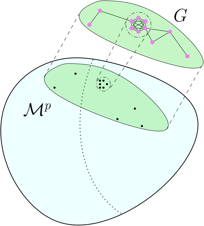
We discuss asymptotics for a fixed number of cliques ($K$) of size $\ell$ where the clique size grows, $\ell\to\infty$. In the appendix (Section C), we discuss the rate of clique formation as well as other alternatives to the clique-based estimators, which can be tailored to sparse graphs. Under this model, as $n\to\infty$, the expected number of cliques of size $\ell=\mathcal{O}(n^{1/(p+2)-\epsilon})$ for $\epsilon>0$ grows to infinity as well. Since the formation of cliques requires nodes to be extremely close to one another in the latent space, the primary driver is the intrinsic dimension of the latent space $p$, rather than the curvature. A formal statement of this is found in the appendix (Section C.3).

An important aspect we consider is the maximum radius of a set of positions conditional on a clique. Unless latent positions are nearly (or exactly) in the same location, large cliques are rare in latent distance models. Lemma 7 illustrates a rate of convergence of these latent locations relative to the size of a clique. Additionally, the nodes which form cliques will also have random effects approaching $0$, Lemma 14.

Under this model, the nodes within a clique have nearly the same latent position. For illustration purposes, we first assume that this holds and later illustrate the rate at which the diameter of the set of latent positions within a clique converges. Let $X,Y\in\{1,2,\dots,n\}$ denote sets of nodes representing non-overlapping cliques. Then the average probability of connection can be used to identify the latent distance if we can also estimate the average of random effects ($\nu$). Let $|W|$ denote the size of $W\in\{X,Y\}$.

See the supplementary materials Section A.6 for the proof of this lemma. The main implication is that it is reasonable to treat the latent positions as a single point when nodes are within a clique. The assumption of $F_{Z}$ admitting a smooth continuous density ($f_{z}$) is extremely mild. In fact, one could derive even faster rates if the latent density contained point masses.

An similar result can be derived for the node-level random effects.

This theorem states that the nodes we find in a clique tend to have near-zero random effects. This will be useful as the random effects will converge to zero, allowing one to use between-clique connections to estimate distances. We next leverage each of these results to construct an estimator for a set of distances on the underlying manifold.

Due to the localization of the latent positions and random effects within a clique, one can estimate a set of distances using the average connection probability across cliques. Let $\mathpzc{X},\mathpzc{Y}\subseteq V$ be subsets of vertices that denote nodes that form cliques respectively. We define the average probability of connection across cliques $\mathpzc{X},\mathpzc{Y}$ by $p_{\mathpzc{X}\mathpzc{Y}}$. Based on the results of Lemma 7, we note that the maximum distance between a set of two points within the same clique is $o_{P}(\exp(-\widetilde{\mu}_{d}\ell))$, therefore we let $d_{\mathpzc{X}\mathpzc{Y}}$ denote the average distance in the latent space between latent positions of the cliques. For any $x,y\in\mathpzc{X},\mathpzc{Y}$, $d_{xy}=d_{\mathpzc{X}\mathpzc{Y}}+o_{P}(\exp(-\widetilde{\mu}_{d}\ell)$ and hence the pairwise distances between nodes in a clique are nearly identical. We can therefore relate the average connection probability to the average distance across cliques:

Since there are $\ell^{2}$ possible connections between a pair of cliques of size $\ell$, we can construct an asymptotically normal estimator of $p_{\mathpzc{X}\mathpzc{Y}}$ using the sample mean of the connections across cliques. By Lemma 7, the distance between latent positions within a clique is negligible. Our goal is to develop an asymptotically normal estimate of $d_{\mathpzc{X}\mathpzc{Y}}$. We can achieve this by estimating $\gamma{X}$ and $\gamma{Y}$ at sufficiently fast rates (i.e., at least $o_{P}(\frac{1}{\ell}))$ so that these are negligible compared to the estimation of $p_{\mathpzc{X}\mathpzc{Y}}$, for which we can leverage a central limit theorem.

For $\mathpzc{W}\in\{\mathpzc{X},\mathpzc{Y}\}$, in order to estimate $\gamma_{\mathpzc{W}}$, we consider the average connection probability to any node in the network, conditional on a node being in a clique of size $\ell$:

By Lemma 7 $d(Z_{i},Z_{j})=o_{P}(\exp(-\widetilde{\mu}_{d}\ell))$. Estimation is straightforward by considering the density of connections, namely: $\widehat{P}(A_{ik}=1|C_{\ell})=\frac{d_{i}}{n}$. Since we only use the ratio to compute the estimates of $\exp(\nu_{i}-\nu_{j})$, the total number of nodes $n$ is not necessary. Given $\ell\ll n$, where $n$ is the number of nodes in the network, this ratio can be estimated easily using the degree ratio. We define $\Delta\nu_{i}:=\nu_{i}-\nu{W}$, allowing us to identify $\Delta\nu_{i}$, where $\nu{W}=\max_{i\in\mathpzc{W}}\nu_{i}$

The remaining question is to estimate $\nu{W}$. Fortunately, as we have previously discussed in Lemma 8, within a clique, the random effects approaches $0$ at an exponentially fast rate. Hence, an estimator for the random effect can be constructed by setting the largest degree node’s random effect to $0$:

This in turn can be used to estimate the distances:

where $\widehat{p}_{\mathpzc{X}\mathpzc{Y}}=\frac{1}{|\mathpzc{X}||\mathpzc{Y}|}\sum_{x\in\mathpzc{X}}\sum_{y\in\mathpzc{Y}}A_{xy}$. The asymptotic distribution is next described in Theorem 9.

The condition (F1) simply states that the size of the cliques should grow at a rate slower than $\sqrt{n}$, the total size of the network, which is a very mild assumption. This is to ensure that the asymptotics associated with the estimation of $\gamma{W}$ are negligible. Condition (F2) is the standard Lindeberg CLT condition. If the node-level probabilities of connection $p_{xy}$ is bounded away from $0$ and $1$, then this will hold (this may not hold if $d_{\mathpzc{X}\mathpzc{Y}}\to-\infty$). The full proof is found in Section A.8. The main implication is that the asymptotic distribution is driven by the estimator $\widehat{p}_{\mathpzc{X}\mathpzc{Y}}$. Since the random effects will approach $0$, for large cliques $p_{\mathpzc{X}\mathpzc{Y}}\approx\exp(-d_{\mathpzc{X}\mathpzc{Y}})$, thus allowing for simplified expressions for $\sigma_{\ell}$ and $p_{\mathpzc{X}\mathpzc{Y}}$.

Constrained Estimation. Pairwise estimation of the distances according to equation (12) is one method of estimating a distance matrix, however, this does not restrict the final estimate to be a metric. When cliques are not connected to one-another, this may result in distance estimates which are $-\infty$.

For example, we construct an enumeration of the cliques of size $7$ or greater from the General Relativity co-authorship network of Leskovec et al. 2007 in Figure 6. Any pair of cliques which does not share an edge will inherently be estimated to have infinite distance, which prevents the estimation of curvature.

To address this challenge, we posit a similar estimation problem, while respecting the triangle inequality for each triplet. The following estimation problem is posed below. Let $\mathcal{C}$ denote the set of cliques in an observed graph. Let $\mathpzc{X}\subset\mathcal{C}$ be a set of indices corresponding to a clique. We estimate the random effects within a clique $i\in\mathpzc{X}$ according to $\widehat{\nu_{i}}=\log(\frac{d_{i}}{\max_{j\in\mathpzc{X}}d_{j}})$. Given a set of fixed effects, we can propose a maximum likelihood optimization problem for the distance matrix $D\in\mathbb{R}^{K\times K}$. As by Lemma 7 cliques have approximately a common latent position. From our latent distance model, we define the following likelihood function for the connections within our set of cliques $\mathcal{C}$, $\mathcal{L}_{\mathcal{C}}$:

We can now define the maximum likelihood optimization problem, after estimating a set of random effects $\boldsymbol{\widehat{\nu}}$

where $\mathcal{C}$ is a list of clique indices. $E_{s}$ are matrices which define the triangle inequalities and contain mostly $0$’s other than $3$ indices, $i,j,k$ for which $E[i,j]=E[i,k]=1=-E[j,k]$. We define $\mathcal{S}$ to be an enumeration of all such matrices $E_{s}$. There are $3\binom{K}{3}$ such restrictions in total. The set of feasible distance matrices that satisfy these constraints form a polyhedron of interior dimension $\binom{K}{2}$, therefore therefore the constraints do not reduce the dimensionality of the space of distance matrices, but reduce the volume of the space to a smaller polyhedron. This optimization procedure is a convex and in practice, we may use CVXR to solve this system (Fu et al. 2020). For a greater gain in computational speed, we use the MOSEK solver for the constrained optimization (Andersen and Andersen 2000).

Though in its current form, the problem is numerically challenging to solve due to the sheer number of constraints. A natural option is to use the Newton method and approximate the likelihood using a second order Taylor expansion and solve this problem successively. Since the Hessian is diagonal, $\frac{\partial^{2}}{\partial d_{ij}\partial d_{kl}}\mathcal{L}_{\mathcal{C}}(D;\boldsymbol{\nu})=0$ if $d_{ij}\not=d_{kl}$, this can be made into a more efficient quadratic program which can be solved faster in CVXR. Let $\widetilde{g}(D;D_{0};\boldsymbol{\nu})$ be the second order Taylor series approximation to $\mathcal{L}_{\mathcal{C}}$ about a matrix $D_{0}$. We can successively solve for $\boldsymbol{\widehat{D}}_{t+1}$ using the following constrained optimization problem

References

- Aliverti and Durante [2019] E. Aliverti and D. Durante. Spatial modeling of brain connectivity data via latent distance models with nodes clustering. Statistical Analysis and Data Mining: The ASA Data Science Journal, 12(3):185–196, 6 2019. ISSN 1932-1872. doi: 10.1002/SAM.11412. URL https://onlinelibrary.wiley.com/doi/full/10.1002/sam.11412.
- Andersen [1970] E. B. Andersen. Asymptotic properties of conditional maximum-likelihood estimators. Journal of the Royal Statistical Society: Series B (Methodological), 32(2):283–301, 1970.
- Andersen and Andersen [2000] E. D. Andersen and K. D. Andersen. The mosek interior point optimizer for linear programming: an implementation of the homogeneous algorithm. In High performance optimization, pages 197–232. Springer, 2000.
- Banerjee et al. [2013] A. Banerjee, A. G. Chandrasekhar, E. Duflo, and M. O. Jackson. The Diffusion of Microfinance. Science, 341(6144), 2013. ISSN 10959203. doi: 10.1126/SCIENCE.1236498.
- Barkanass et al. [2022] V. Barkanass, U. Jost, and E. Hancock. Geometric sampling of networks. Journal of Complex Networks, 10(4), 6 2022. ISSN 2051-1310. doi: 10.1093/COMNET/CNAC014. URL https://academic.oup.com/comnet/article/10/4/cnac014/6644814.
- Bassett et al. [2018] D. S. Bassett, P. Zurn, and J. I. Gold. On the nature and use of models in network neuroscience. Nature Reviews Neuroscience 2018 19:9, 19(9):566–578, 7 2018. ISSN 1471-0048. doi: 10.1038/s41583-018-0038-8. URL https://www.nature.com/articles/s41583-018-0038-8.
- Begelfor and Werman [2005] E. Begelfor and M. Werman. The World is not always Flat or Learning Curved Manifolds. School of Engineering and Computer Science, Hebrew University of Jerusalem., Tech. Rep, 3(8), 2005.
- Berger [1962] M. Berger. An extension of rauch’s metric comparison theorem and some applications. Illinois Journal of Mathematics, 6(4):700–712, 1962.
- Blumenthal and Gillam [1943] L. M. Blumenthal and B. E. Gillam. Distribution of Points in n-Space. The American Mathematical Monthly, 50(3):181, 3 1943. ISSN 00029890. doi: 10.2307/2302400.
- Borgatti et al. [2009] S. P. Borgatti, A. Mehra, D. J. Brass, and G. Labianca. Network analysis in the social sciences. Science, 323(5916):892–895, 2 2009. ISSN 00368075. doi: 10.1126/SCIENCE.1165821/ASSET/2421E2F8-2DC7-4CAD-8A84-471B43A3C443/ASSETS/GRAPHIC/323˙892˙F5.JPEG. URL https://www.science.org/doi/10.1126/science.1165821.
- Brauchart et al. [2015] J. S. Brauchart, A. B. Reznikov, E. B. Saff, I. H. Sloan, Y. G. Wang, and R. S. Womersley. Random Point Sets on the Sphere — Hole Radii, Covering, and Separation. Experimental Mathematics, 27(1):62–81, 12 2015. ISSN 1944950X. doi: 10.1080/10586458.2016.1226209. URL https://arxiv.org/abs/1512.07470v2.
- Burt [1992] R. S. Burt. Structural holes: The social structure of competition. Harvard University Press, Cambridge, MA, 1992.
- Buskens and Van de Rijt [2008] V. Buskens and A. Van de Rijt. Dynamics of networks if everyone strives for structural holes. American Journal of Sociology, 114(2):371–407, 2008.
- Cai et al. [2013] T. Cai, J. Fan, and T. Jiang. Distributions of Angles in Random Packing on Spheres. Journal of Machine Learning Research, 14:1837–1864, 2013.
- Chamberlain et al. [2017] B. P. Chamberlain, J. R. Clough, and M. P. Deisenroth. Neural Embeddings of Graphs in Hyperbolic Space. In 13th international workshop on mining and learning from graphs held in conjunction with KDD, 2017.
- Chami et al. [2019] I. Chami, R. Ying, C. Ré, and J. Leskovec. Hyperbolic Graph Convolutional Neural Networks. Advances in Neural Information Processing Systems, 32, 10 2019. ISSN 10495258. doi: 10.48550/arxiv.1910.12933. URL https://arxiv.org/abs/1910.12933v1.
- Chen et al. [2021] M. Chen, K. Kato, and C. Leng. Analysis of networks via the sparse -model. Journal of the Royal Statistical Society Series B: Statistical Methodology, 83(5):887–910, 2021.
- Csardi et al. [2006] G. Csardi, T. Nepusz, et al. The igraph software package for complex network research. InterJournal, complex systems, 1695(5):1–9, 2006.
- Durante et al. [2013] F. Durante, J. Fernández-Sánchez, and C. Sempi. A topological proof of Sklar’s theorem. Applied Mathematics Letters, 26(9):945–948, 9 2013. ISSN 0893-9659. doi: 10.1016/J.AML.2013.04.005.
- Farooq et al. [2019] H. Farooq, Y. Chen, T. T. Georgiou, A. Tannenbaum, and C. Lenglet. Network curvature as a hallmark of brain structural connectivity. Nature Communications 2019 10:1, 10(1):1–11, 10 2019. ISSN 2041-1723. doi: 10.1038/s41467-019-12915-x. URL https://www.nature.com/articles/s41467-019-12915-x.
- Fearnhead and Rigaill [2016] P. Fearnhead and G. Rigaill. Changepoint Detection in the Presence of Outliers. Journal of the American Statistical Association, 114(525):169–183, 9 2016. ISSN 1537274X. doi: 10.48550/arxiv.1609.07363. URL https://arxiv.org/abs/1609.07363v2.
- Fosdick et al. [2016] B. K. Fosdick, T. H. McCormick, T. B. Murphy, T. L. J. Ng, and T. Westling. Multiresolution network models. Journal of Computational and Graphical Statistics, 28(1):185–196, 8 2016. ISSN 15372715. doi: 10.48550/arxiv.1608.07618. URL https://arxiv.org/abs/1608.07618v5.
- Frechet [1957] M. Frechet. Sur la distance de deux lois de probabilite. CR. Acad Sci. Paris, 244, 1957.
- Fu et al. [2020] A. Fu, B. Narasimhan, and S. Boyd. CVXR: An R package for disciplined convex optimization. Journal of Statistical Software, 94(14):1–34, 11 2020. ISSN 15487660. doi: 10.18637/jss.v094.i14. URL https://CRAN.R-project.
- Gallot et al. [2004] S. Gallot, D. Hulin, and J. Lafontaine. Riemannian Geometry. Universitext. Springer Berlin Heidelberg, Berlin, Heidelberg, 2004. ISBN 978-3-540-20493-0. doi: 10.1007/978-3-642-18855-8. URL http://link.springer.com/10.1007/978-3-642-18855-8.
- Gilbert and Jain [2017] A. C. Gilbert and L. Jain. If it ain’t broke, don’t fix it: Sparse metric repair. In 2017 55th Annual Allerton Conference on Communication, Control, and Computing (Allerton), pages 612–619. IEEE, 2017.
- Grimmett and McDiarmid [1975] G. R. Grimmett and C. J. McDiarmid. On colouring random graphs. In Mathematical Proceedings of the Cambridge Philosophical Society, volume 77, pages 313–324. Cambridge University Press, 1975.
- Gromov [2007] M. Gromov, editor. Metric Structures for Riemannian and NonRiemannian Spaces. Birkhäuser Boston, 2007. doi: 10.1007/978-0-8176-4583-0.
- Gu et al. [2018] A. Gu, F. Sala, B. Gunel, and C. Ré. Learning mixed-curvature representations in product spaces. In International Conference on Learning Representations, 2018.
- Handcock et al. [2007] M. S. Handcock, A. E. Raftery, and J. M. Tantrum. Model-based clustering for social networks. Journal of the Royal Statistical Society: Series A (Statistics in Society), 170(2):301–354, 3 2007. ISSN 1467-985X. doi: 10.1111/J.1467-985X.2007.00471.X. URL https://onlinelibrary.wiley.com/doi/full/10.1111/j.1467-985X.2007.00471.xhttps://onlinelibrary.wiley.com/doi/abs/10.1111/j.1467-985X.2007.00471.xhttps://rss.onlinelibrary.wiley.com/doi/10.1111/j.1467-985X.2007.00471.x.
- Harchaoui and Lévy-Leduc [2010] Z. Harchaoui and C. Lévy-Leduc. Multiple change-point estimation with a total variation penalty. Journal of the American Statistical Association, 105(492):1480–1493, 2010.
- Havel and Wüthrich [1985] T. F. Havel and K. Wüthrich. An evaluation of the combined use of nuclear magnetic resonance and distance geometry for the determination of protein conformations in solution. Journal of molecular biology, 182(2):281–294, 1985.
- Hoeffding [1940] W. Hoeffding. Masstabvariarte Korrelationstheorie. Schrijl Math. Inst. Univ. Berlin, 5(6), 1940.
- Hoff [2007] P. Hoff. Modeling homophily and stochastic equivalence in symmetric relational data. Advances in neural information processing systems, 20, 2007.
- Hoff et al. [2002] P. D. Hoff, A. E. Raftery, and M. S. Handcock. Latent space approaches to social network analysis. Journal of the american Statistical association, 97(460):1090–1098, 2002.
- Hopf [1926] H. Hopf. Zum clifford-kieinschen raumproblem. Mathematische Annalen, 95:313–339, 1926.
- Killing [1891] W. Killing. Ueber die Clifford-Klein’schen Raumformen. Mathematische Annalen 1891 39:2, 39(2):257–278, 6 1891. ISSN 1432-1807. doi: 10.1007/BF01206655. URL https://link.springer.com/article/10.1007/BF01206655.
- Kim et al. [2018] B. Kim, K. H. Lee, L. Xue, and X. Niu. A review of dynamic network models with latent variables. Statistics surveys, 12:105, 2018.
- Klingenberg [1995] W. Klingenberg. Riemannian Geometry. Walter de Gruyter, 1 edition, 12 1995. doi: 10.1515/9783110905120.
- Kusner et al. [2015] M. Kusner, Y. Sun, N. Kolkin, and K. Weinberger. From word embeddings to document distances. In International conference on machine learning, pages 957–966. PMLR, 2015.
- Le Cam [1956] L. Le Cam. On the asymptotic theory of estimation and testing hypotheses. In Proceedings of the Third Berkeley Symposium on Mathematical Statistics and Probability, Volume 1: Contributions to the Theory of Statistics, volume 3, pages 129–157. University of California Press, 1956.
- Leal et al. [2018] W. Leal, G. Restrepo, P. F. Stadler, and J. Jost. Forman-Ricci Curvature for Hypergraphs. Advances in Complex Systems, 24(1), 11 2018. doi: 10.13140/RG.2.2.27347.84001. URL http://arxiv.org/abs/1811.07825http://dx.doi.org/10.13140/RG.2.2.27347.84001.
- Lee et al. [2019] W. Lee, T. H. Mccormick, J. Neil, M. Cole, S. Microsoft, and Y. Cui. Anomaly Detection in Large Scale Networks with Latent Space Models. Technometrics, pages 1–23, 11 2019. ISSN 0040-1706. doi: 10.1080/00401706.2021.1952900. URL https://arxiv.org/abs/1911.05522v2.
- Leskovec et al. [2007] J. Leskovec, J. Kleinberg, and C. Faloutsos. Graph evolution. ACM Transactions on Knowledge Discovery from Data (TKDD), 1(1), 3 2007. ISSN 15564681. doi: 10.1145/1217299.1217301. URL https://dl.acm.org/doi/abs/10.1145/1217299.1217301.
- Li and Dunson [2019] D. Li and D. B. Dunson. Geodesic distance estimation with spherelets. arXiv preprint arXiv:1907.00296, 2019.
- Li et al. [2017] D. Li, M. Mukhopadhyay, and D. B. Dunson. Efficient manifold and subspace approximations with spherelets. arXiv preprint arXiv:1706.08263, 2017.
- Lok et al. [2021] T. Lok, J. Ng, T. B. Murphy, T. Westling, T. H. Mccormick, and B. Fosdick. Modeling the social media relationships of Irish politicians using a generalized latent space stochastic blockmodel. Annals of Applied Statistics, 15(4):1923–1944, 12 2021. ISSN 1932-6157. doi: 10.1214/21-AOAS1483.
- Lubold et al. [2023] S. Lubold, A. G. Chandrasekhar, and T. H. McCormick. Identifying the latent space geometry of network models through analysis of curvature. Journal of the Royal Statistical Society Series B: Statistical Methodology, 2023.
- MacDonald et al. [2022] P. W. MacDonald, E. Levina, and J. Zhu. Latent space models for multiplex networks with shared structure. Biometrika, 109(3):683–706, 2022.
- Nagano et al. [2019] Y. Nagano, S. Yamaguchi, Y. Fujita, and M. Koyama. A Wrapped Normal Distribution on Hyperbolic Space for Gradient-Based Learning. 36th International Conference on Machine Learning, ICML 2019, 2019-June:8242–8251, 2 2019. doi: 10.48550/arxiv.1902.02992. URL https://arxiv.org/abs/1902.02992v2.
- Ni et al. [2019] C. C. Ni, Y. Y. Lin, F. Luo, and J. Gao. Community Detection on Networks with Ricci Flow. Scientific Reports 2019 9:1, 9(1):1–12, 7 2019. ISSN 2045-2322. doi: 10.1038/s41598-019-46380-9. URL https://www.nature.com/articles/s41598-019-46380-9.
- Nickel and Kiela [2017] M. Nickel and D. Kiela. Poincaré Embeddings for Learning Hierarchical Representations. Advances in Neural Information Processing Systems, 30, 2017.
- Ollivier [2007] Y. Ollivier. Ricci curvature of Markov chains on metric spaces. Journal of Functional Analysis, 256(3):810–864, 1 2007. ISSN 00221236. doi: 10.48550/arxiv.math/0701886. URL https://arxiv.org/abs/math/0701886v4.
- Papadopoulos et al. [2018] L. Papadopoulos, M. A. Porter, K. E. Daniels, and D. S. Bassett. Network analysis of particles and grains. Journal of Complex Networks, 6(4):485–565, 8 2018. ISSN 20511329. doi: 10.1093/COMNET/CNY005. URL https://academic.oup.com/comnet/article/6/4/485/4959635.
- Pennec [1999] X. Pennec. Probabilities and statistics on Riemannian manifolds: Basic tools for geometric measurements. In International Workshop on Nonlinear Signal and Image Processing, pages 194–198, Antalya, Turkey, 6 1999. URL http://www-sop.inria.fr/epidaure/personnel/pennec/pennec.html.
- Politis and Romano [1994] D. N. Politis and J. P. Romano. Large Sample Confidence Regions Based on Subsamples under Minimal Assumptions. https://doi.org/10.1214/aos/1176325770, 22(4):2031–2050, 12 1994. ISSN 0090-5364. doi: 10.1214/AOS/1176325770.
- Salter-Townshend and McCormick [2017] M. Salter-Townshend and T. H. McCormick. Latent space models for multiview network data. Annals of Applied Statistics, 11(3):1217–1244, 9 2017. ISSN 1932-6157. doi: 10.1214/16-AOAS955. URL https://projecteuclid.org/journals/annals-of-applied-statistics/volume-11/issue-3/Latent-space-models-for-multiview-network-data/10.1214/16-AOAS955.full.
- Samal et al. [2021] A. Samal, H. K. Pharasi, S. J. Ramaia, H. Kannan, E. Saucan, J. Jost, and A. Chakraborti. Network geometry and market instability. Royal Society Open Science, 8(2), 2 2021. ISSN 20545703. doi: 10.1098/RSOS.201734. URL https://royalsocietypublishing.org/doi/10.1098/rsos.201734.
- Sandhu et al. [2015] R. Sandhu, T. Georgiou, E. Reznik, L. Zhu, I. Kolesov, Y. Senbabaoglu, and A. Tannenbaum. Graph Curvature for Differentiating Cancer Networks. Nature Scientific Reports, 5(1):1–13, 7 2015. ISSN 2045-2322. doi: 10.1038/srep12323. URL https://www.nature.com/articles/srep12323.
- Sandhu et al. [2016] R. S. Sandhu, T. T. Georgiou, and A. R. Tannenbaum. Ricci curvature: An economic indicator for market fragility and systemic risk. Science Advances, 2(5), 5 2016. ISSN 23752548. doi: 10.1126/SCIADV.1501495/SUPPL˙FILE/1501495˙SM.PDF. URL https://www.science.org/doi/10.1126/sciadv.1501495.
- Saucan et al. [2020] E. Saucan, A. Samal, and J. Jost. A Simple Differential Geometry for Complex Networks. Network Science, 9(S1):S106–S133, 4 2020. ISSN 20501250. doi: 10.48550/arxiv.2004.11112. URL https://arxiv.org/abs/2004.11112v2.
- Schoenberg [1935] I. J. Schoenberg. Remarks to Maurice Frechet’s Article “Sur La Definition Axiomatique D’Une Classe D’Espace Distances Vectoriellement Applicable Sur L’Espace De Hilbert. The Annals of Mathematics, 36(3):724, 7 1935. ISSN 0003486X. doi: 10.2307/1968654.
- Sia et al. [2019] J. Sia, E. Jonckheere, and P. Bogdan. Ollivier-Ricci Curvature-Based Method to Community Detection in Complex Networks. Nature, Scientific Reports 2019 9:1, 9(1):1–12, 7 2019. ISSN 2045-2322. doi: 10.1038/s41598-019-46079-x. URL https://www.nature.com/articles/s41598-019-46079-x.
- Sklar [1959] A. Sklar. Fonctions de repartition a n dimensions et leurs marges. Publications de l’Institut de statistique de l’Université de Paris, 8:229–231, 1959. URL https://ci.nii.ac.jp/naid/10011938360.
- Smith et al. [2017] A. L. Smith, D. M. Asta, and C. A. Calder. The Geometry of Continuous Latent Space Models for Network Data. Statistical Science, 34(3):428–453, 12 2017. ISSN 21688745. doi: 10.48550/arxiv.1712.08641. URL https://arxiv.org/abs/1712.08641v2.
- Sweet and Adhikari [2020] T. Sweet and S. Adhikari. A Latent Space Network Model for Social Influence. Psychometrika, 85(2):251–274, 6 2020. ISSN 18600980. doi: 10.1007/S11336-020-09700-X/FIGURES/11. URL https://link.springer.com/article/10.1007/s11336-020-09700-x.
- Tenenbaum et al. [2000] J. B. Tenenbaum, V. d. Silva, and J. C. Langford. A global geometric framework for nonlinear dimensionality reduction. science, 290(5500):2319–2323, 2000.
- Torgerson [1952] W. S. Torgerson. Multidimensional scaling: I. theory and method. Psychometrika, 17(4):401–419, 1952.
- van der Hoorn et al. [2020] P. van der Hoorn, W. J. Cunningham, G. Lippner, C. Trugenberger, and D. Krioukov. Ollivier-Ricci curvature convergence in random geometric graphs. Physical Review Research, 3(1), 8 2020. doi: 10.1103/PhysRevResearch.3.013211. URL http://arxiv.org/abs/2008.01209http://dx.doi.org/10.1103/PhysRevResearch.3.013211.
- van der Vaart [1998] A. van der Vaart. Asymptotic Statistics. Cambridge University Press, 10 1998. doi: 10.1017/cbo9780511802256. URL /core/books/asymptotic-statistics/A3C7DAD3F7E66A1FA60E9C8FE132EE1D.
- Volz et al. [2011] E. M. Volz, J. C. Miller, A. Galvani, and L. Meyers. Effects of Heterogeneous and Clustered Contact Patterns on Infectious Disease Dynamics. PLOS Computational Biology, 7(6):e1002042, 2011. ISSN 1553-7358. doi: 10.1371/JOURNAL.PCBI.1002042. URL https://journals.plos.org/ploscompbiol/article?id=10.1371/journal.pcbi.1002042.
- Zhang et al. [2021] S. Zhang, Y. Tay, W. Jiang, D.-c. Juan, and C. Zhang. Switch spaces: learning product spaces with sparse gating. arXiv preprint arXiv:2102.08688, 2021.
Appendix A Proofs of Theorems
A.1 Proof of Lemma 2
In order to prove this lemma, we first introduce a useful result.
Theorem 10 (Theorem 1.10.15 in Klingenberg 1995).
If is an isometry on a Riemannian manifold, then the fixed point set of forms a totally geodesic submanifold.
Using this theorem, if we can construct an isometry, a bijective isomorphism between two metric spaces (in this case, the submanifold within the canonical manifold which contains the triangle, as well as the canonical manifold of dimension 2), then the fixed points of the set will form a totally geodesic submanifold which will be useful for constructing our fixed point equation.
Proof.
We will prove this by first considering constructing a change of basis to parameterize the sub-manifold using the first coordinates, then we will construct the isometry between the manifold of dimension and that of dimension .
Consider a set of 3 points which are not co-linear. We can construct an orthogonal matrix (rotation matrix) which allows us to construct a rotational isometry.
WLOG, in our coordinate system, we place at the origin, i.e. . We construct an orthogonal rotation matrix which rotates the coordinates into the first indices, with the rest of them being . Let denote the un-normalized column vector of , and . We the define the following first basis functions as the normalized projections of the components of and then :
Since are not colinear, then are independent and are the normalization’s of respectively and are orthogonal. The remaining columns of are the completion of the orthonormal basis with any remaining orthogonal basis vectors of . Thus we have constructed an orthogonal matrix and . This matrix can be used to construct an isometry where
Hence, this rotation is an isometry. Therefore, we can equivalently use the parameterization where the points have non-zero coordinates only in the first three indices.
Next, let denote an second mapping. Under this transformation
and thus is also an isometry. Since the composition of isometries is also an isometry. By the composition of this rotation and sign flip of coordinates, we can construct the corresponding totally geodesic submanifold as follows. Lastly the totally geodesic submanifold of dimension can be constructed using the set of points satisfying for for any such that , which is simply a reparameterization of mapped into . By construction of this rotation matrix, are all fixed points of this isometry (). When translating between coordinate positions and the distances, one must use the same curvature value , and thus the totally geodesic manifold of dimension exists with the same curvature, and thus contains its midpoints.
The proofs for and follows this argument identically and thus the proof is complete.
∎
A.2 Proof of Theorem 3
In order to develop our identifying equation for the curvature using triangle distances, we note that any three points can be embedded isometrically in a totally geodesic submanifold of dimension 2 when is a canonical manifold, as stated in Lemma 2. Since this is a totally geodesic submanifold, the distance to the midpoint parameterized by coordinates in will be the same as in . We continue with the proof by embedding the triangle in a canonical manifold of dimension 2. This will provide an implicit equation for the curvature, determined by the side lengths of the triangle as well as the length of the triangle median. In each case, we use the representations of the canonical manifolds outlined in Section 2.1.
Case 1: Spherical. For convenience of derivation, we derive an implicit equation in a coordinate system where the midpoint of points and is placed at the origin ( in ) and the line between and define the axis . Given the distance we place point at the point where . Next we place point at where and . Given this parameterization of the manifold embedding of , and the distances, , we solve for the coordinates of .
In general, . Since the midpoint is placed at , then . Next, can be solved for by considering its distance to :
Similarly the distance to can be computed as:
Solving for leads to the expression
which can be further rearranged as follows:
This finally leads to the expression:
We then normalize this by the curvature value , which allows for to be a continuous function of from the hyperbolic to spherical space .
In the spherical case, we also require that the distances themselves satisfy , due to the fact that this corresponds to the maximum possible distance on the sphere, however this restriction is not present in the and .
Case 2: Hyperbolic. The proof for deriving this method in the hyperbolic case follows an identical method to the spherical case and is left out for brevity. The resultant estimating function is of the following form
Remark: Under the limit as we find that which gives exactly the parallelogram law in Euclidean space. This also highlights the necessity that the term plays in maintaining a smooth equation as a function of through . ∎
A.3 Proof of Theorem 4
We will use the implicit function theorem to construct a function for which we can later apply a delta method. In order to do so, we must ensure that for such that . We first note that is continuously differentiable when . This boundary corresponds to the maximum distance allowed on a sphere, as given by two anti-polar points. Therefore to apply the implicit function theorem, what remains is
which will hold by a brief application of (B3). As we have derived in Theorem 3, , the length of the triangle median as a function of the triangle lengths is a differentiable, continuous, increasing function of .
By definition, this function satisfies
Let denote the fixed value of the triangle median length at value of the true curvature , and let denote the median length as a function of the triangle side length. We can now write the estimating function as a function of the equivalent exact midpoint 11 1 We drop triangle lengths dependence for brevity
We compute the derivative as a function of
Since ,
Since then if then and hence has positive derivative for , where we use the notation when we are specifying the as a function of for a fixed set of distances.
Next, by the implicit function theorem, there exists an open neighborhood and an “implicit” function such that: and for . Furthermore the gradient satisfies:
Therefore by the delta method we arrive at the asymptotic distribution of
where refers to convergence in distribution. Lastly, by the implicit function theorem:
If instead we only have consistency, rather than asymptotic normality of , , then we can use the continuous mapping theorem instead and we have . Remark: This form is very similar to the usual standard asymptotic normality proofs for estimators as in van der Vaart 1998. However, the main difference is in the fact that we are not averaging the estimating function, but rather plugging in a distance estimate which is asymptotically normal, meaning that we develop this delta method argument for a plug-in estimator.
We find that in practice, condition (B3) holds quite generally, unless the points are co linear. In fact, in the Euclidean case, we can derive this exactly according to the Taylor series expansion at
Clearly at the solution reduces to the parallelogram law . When we substitute in the corresponding solution at
As long as the triangle inequality is satisfied strictly for , then . However, if the triangle inequality is not strict, i.e. are co-linear, and for being some permutation of , then . For , we do not have simple closed-form expressions for and thus we leave (B3) as an assumption, however, we believe this pattern to hold in the other canonical manifolds.
Lemma 11.
If , let denote the midpoint between and . Then let denote the distance to the midpoint from as a function of the curvature of the latent space .
Then is a non-decreasing function in .
The proof follows from Toponogov’s triangle theorem and the negative curvature extension [Berger 1962] which we include immediately following this proof in Theorem 12. Abbreviated for our purposes in Theorem 12, we simply let and compare two manifolds .
Then it immediately follows
Theorem 12 (Toponogov’s Triangle Comparison Theorem (Theorem 3 of Berger 1962).
Let be a complete Riemannian manifold, and let be the simply connected manifold of constant curvature . Let denote a geodesic triangle with points . Let is the geodesic triangle with side lengths and on . If is the minimum Riemannian sectional curvature on the manifold, and if , then
This theorem suggests that assumption (B3) is therefore very mild and that we will always have a non-decreasing function of but that we only have to assume that the increasingness is strict. In practice, we observe this is only not strict when the points are co-linear, and therefore the distance to the midpoint does not change as a function of the curvature since, effectively, these points lie along a single geodesic.
A.4 Proof of Theorem 5
Recall that denotes the vector of the distances of the triangle with vertices , and let be the distances in triangle . We also measure the distance to the surrogate midpoint, . Though we do not have access to the distance to the true midpoint , this is going to be a function of the curvature of the space, and the distances of the triangle and the median length . For any curvature and a surrogate midpoint , so that , we can upper and lower bound the triangle median length. By the triangle inequality these upper and lower bounds are
By Lemma 11 each function is monotone in . The upper and lower bounds can then be computed by plugging in this value to , i.e. and solving for . By this monotonicity, the number of solutions in to either equation will typitcally be .
If there is a solution to , then we have found and upper and lower bounds. If there are no solutions, then the upper and lower bounds are . In the event that there are colinear points, then this can lead to a situation where has multiple solutions in . In this case, we can take the minimum of the upper bounds and maximum of the lower bounds respectively. ∎
A.5 Proof of Theorem 6
Before proving Theorem 6, we first introduce a useful theorem for the proof.
Theorem 13.
Consider a set of continuous random variables which are marginally identical but have an arbitrary dependency. Let denote the sample median of the set of these random variables. Then