Autonomous Satellite Rendezvous and Proximity Operations with Time-Constrained Sub-Optimal Model Predictive ControlApproved for public release; distribution is unlimited. Public Affairs approval #AFRL-2022-5517.GB and MH were supported by AFOSR under grant FA9550-19-1-0169, ONR under grants N00014-19-1-2543, N00014-21-1-2495, and N00014-22-1-2435, and AFRL under grants FA8651-22-F-1052 and FA8651-08-D-0108 TO48.

Gabriel Behrendt Alexander Soderlund Matthew Hale Sean Phillips Address: University of Florida, Gainesville, FL 32611 USA (e-mail: gbehrendt@ufl.edu). Address: Space Vehicles Directorate, Air Force Research Laboratory, Kirtland AFB, NM 87108 USA (e-mail: alexander.soderlund.1@spaceforce.mil). Address: University of Florida, Gainesville, FL 32611 USA (e-mail: matthewhale@ufl.edu). Address: Space Vehicles Directorate, Air Force Research Laboratory, Kirtland AFB, NM 87108 USA (e-mail: sean.phillips.9@spaceforce.mil).

Abstract

This paper presents a time-constrained model predictive control strategy for the 6 degree-of-freedom (6DOF) autonomous rendezvous and docking problem between a controllable “deputy” spacecraft and an uncontrollable “chief” spacecraft. The control strategy accounts for computational time constraints due to limited onboard processing speed. The translational dynamics model is derived from the Clohessy-Wiltshire equations and the angular dynamics are modeled on gas jet actuation about the deputy’s center of mass. Simulation results are shown to achieve the docking configuration under computational time constraints by limiting the number of allowed algorithm iterations when computing each input. Specifically, we show that upwards of $\mathchar 28729\mathchar 28720$ % of computations can be eliminated from a model predictive control implementation without significantly harming control performance.

keywords

Aerospace, Autonomous systems, Real-time optimal control

1 Introduction

Autonomy has become increasingly necessary for space applications due to the growing number of deployed satellites and limited ability to use human-in-the-loop control (ESA 2022). The autonomous rendezvous and docking (ARPOD) problem is one of these applications which has gained significant interest because of recent space missions such as the NASA DART mission (Cheng et al. 2018) and its uses in applications such as satellite inspection (Bernhard et al. 2020) and servicing (Ogilvie et al. 2008). In general, the ARPOD problem requires a deputy spacecraft to maneuver to a desired state relative to a chief spacecraft.

There are a few challenges that must be addressed in the ARPOD problem to design a reliable and practically-implementable control strategy. One challenge is that the dynamics of the satellites are nonlinear when both the translational and attitude dynamics are considered together. Another challenge is that these models are subject to disturbances such as sensor noise, model mismatch, and others unique to operations in space, such as J2 perturbations and solar pressure. Furthermore, in the design of a control strategy, we must consider that input commands must be computed using space-grade hardware. Since space-grade processors must be radiation-hardened (which requires lengthy construction cycles) to handle the electronics-hostile space environment (Bourdarie and Xapsos 2008) and the design of space missions are often multi-year endeavors, there is a sizable processing capabilities gap between state-of-the-art, commercial off-the-shelf CPUs and their space-grade counterparts (Lovelly and George 2017; Lovelly 2017). A challenge of this computational gap is that space-based missions are becoming increasingly complex, particularly in the congested low-Earth orbit domain. Thus, we require a control strategy that (i) can handle nonlinearities in dynamics, (ii) is robust to perturbations, and (iii) can be computed by a computationally-limited satellite.

Often, autonomous control problems are solved via state feedback methods. Model predictive control (MPC) has been widely utilized (Falcone et al. 2007) and is a natural fit for the ARPOD problem due to its robustness and ability to handle nonlinearities. In conventional MPC, an optimization problem is solved at each time step to completion, i.e., a new control input is computed by solving an optimization problem until a stopping condition is reached. However, given the limited available computational speed in space, we cannot reliably use conventional MPC new inputs to the system may be needed before the computations to find those inputs can be completed.

Therefore, in this work, we use a method that we refer to as time-constrained MPC. We consider a setting in which the underlying optimization algorithm is only allowed enough time to complete a limited number of iterations when computing each input. This constraint only allows the algorithm to make some progress toward the optimum, and, when the time constraint is reached, a sub-optimal input is applied to the system by using the optimization algorithm’s most recent iterate.

It is known in the MPC literature that the optimization problem does not need to be solved to completion in order to ensure stability of the solution (Mayne 2014; Graichen and Käpernick 2012; Graichen and Kugi 2010; Pavlov et al. 2019). These works suggest that time-constrained MPC is a viable solution to account for nonlinear dynamics, perturbations, and limited onboard computational speed seen in the ARPOD problem, and this paper formalizes and confirms this point.

1.1 Summary of Contributions

To summarize, the contributions of this paper are:

1.

Modeling of the ARPOD problem considering both translational and attitude dynamics
2.

Empirical validation that time-constrained MPC succeeds in docking for the 6 DoF ARPOD problem
3.

Empirical validation that time-constrained MPC succeeds in docking for the fully actuated 6 DoF ARPOD problem with perturbations
4.

Comparison of performance under different computation constraints and validation that more than $\mathchar 28729\mathchar 28720$ % of computations can be eliminated in the ARPOD problem without significantly harming performance

1.2 Related Work

The ARPOD problem has been studied in a variety of settings. Some works have considered only controlling translational (Jewison 2017) or attitudinal dynamics (Leomanni et al. 2014; Trivailo et al. 2009). Typically, ARPOD studies consider translational control inputs that are uncoupled from the attitudinal dynamics, such as in (Hogan and Schaub 2014). While recent studies (Soderlund et al. 2021; Soderlund and Phillips 2022) have considered coupled translational-attitudinal systems, only two-dimensional motion between the deputy and chief was considered. Other works have developed control strategies for the more complex three-dimensional 6DOF ARPOD problem with coupled translational and attitude dynamics. These works include approaches from nonlinear control such as back-stepping (Sun and Huo 2015; Wang and Ji 2019), sliding mode (Yang and Stoll 2019; Zhou et al. 2020), learning-based control (Hu et al. 2021), and artificial potential functions (Dong et al. 2018). This paper differs from those earlier works in that we do not use a static control law with user-defined gains. Instead, we use MPC to solve for our next control input.

Model Predictive Control has been used for the 3 degree-of-freedom ARPOD problem while considering various constraints, such as collision avoidance and line-of-sight constraints (Petersen et al. 2014; Li et al. 2017; Wang et al. 2018; Richards and How 2003; Di Cairano et al. 2012). Considering only the translational dynamics can be convenient because, under mild assumptions, the dynamics are linear. (Lee and Mesbahi 2017) also considers a dual-quaternion formulation of the 6DOF ARPOD problem, and they use a piecewise affine approximation of the nonlinear system model so that the MPC problem can be solved quickly onboard (Hartley 2015). Other computational considerations include using a pre-computed lookup table (Malyuta et al. 2021), or designing custom predictive controller hardware (Hartley and Maciejowski 2013). In this paper, we differ because we consider a nonlinear dynamic model without any approximation and we explicitly address computational time constraints.

The rest of the paper is organized as follows. Section 2 presents preliminaries. Then Section 3 gives a time-constrained MPC problem statement. After that, Section 4 provides simulation results, and Section 5 concludes.

2 Preliminaries

The Euclidean $\mathchar 29038$ -dimensional space is denoted by $\mathbb{\mathchar 29010}^{\mathchar 29038}$ . The vector $\delimiter 69640972\mathchar 12850\mathbb{\mathchar 29010}^{\mathchar 29038}$ is defined as $\delimiter 69640972\mathchar 12346\mathchar 12349\delimiter 67273472\delimiter 69640972_{\mathchar 28721}\mathchar 24891\dots\mathchar 24891\delimiter 69640972_{\mathchar 29038}\delimiter 84054785^{\mathchar 574}$ , where the superscript $\mathchar 574$ denotes the transpose operation. Unless otherwise specified, all vectors used in this paper are physical vectors, meaning that they exist irrespective of any coordinate frame used. For instance, the vector $\delimiter 69640972^{\mathcal{\mathchar 28993}}$ denotes that the vector is given by the coordinates defined by the frame $\mathcal{\mathchar 28993}$ , while $\delimiter 69640972^{\mathcal{\mathchar 28994}}$ denotes that the vector is given by the coordinates defined by the frame $\mathcal{\mathchar 28994}$ . For $\delimiter 69640972\mathchar 12850\mathbb{\mathchar 29010}^{\mathchar 28723}$ , $\delimiter 67482370\delimiter 69640972\delimiter 84267779^{\mathchar 8706}$ denotes the skew-symmetric operator, i.e.,

\delimiter 67482370\delimiter 69640972\delimiter 84267779^{\mathchar 8706}\mathchar 12349\begin{\mathchar29026\mathchar29037\mathchar29025\mathchar29044\mathchar29042\mathchar29033\mathchar29048}\mathchar 28720&\mathchar 8704\delimiter 69640972_{\mathchar 28723}&\delimiter 69640972_{\mathchar 28722}\\ \delimiter 69640972_{\mathchar 28723}&\mathchar 28720&\mathchar 8704\delimiter 69640972_{\mathchar 28721}\\ \mathchar 8704\delimiter 69640972_{\mathchar 28722}&\delimiter 69640972_{\mathchar 28721}&\mathchar 28720\end{\mathchar29026\mathchar29037\mathchar29025\mathchar29044\mathchar29042\mathchar29033\mathchar29048}\mathchar 314

(1)

The $\mathchar 29038\mathchar 8706\mathchar 29038$ identity matrix is denoted by $\mathchar 29001_{\mathchar 29038}$ , while $\textbf{0}_{\mathchar 29038}$ denotes the zero column vector with dimension $\mathchar 29038\mathchar 8706\mathchar 28721$ . Similarly, the $\mathchar 29038\mathchar 8706\mathchar 28721$ -dimensional column vector of ones is denoted by $\textbf{1}_{\mathchar 29038}$ . The $\mathchar 29038$ -dimensional multivariate normal distribution is denoted $\mathcal{\mathchar 29006}\delimiter 67273472\mathchar 28967\mathchar 24891\mathchar 28955\delimiter 84054785$ , where $\mathchar 28967\mathchar 12850\mathbb{\mathchar 29010}^{\mathchar 29038}$ is the mean and $\mathchar 28955\mathchar 12850\mathbb{\mathchar 29010}^{\mathchar 29038\mathchar 8706\mathchar 29038}$ is the covariance matrix.

The Lie Group $\mathbf{\mathchar 29011\mathchar 29007}\delimiter 67273472\mathchar 28723\delimiter 84054785$ is the set of all real invertible $\mathchar 28723\mathchar 8706\mathchar 28723$ matrices that are orthogonal with determinant $\mathchar 28721$ , i.e.,

{\mathbf{\mathchar 29011\mathchar 29007}}\delimiter 67273472\mathchar 28723\delimiter 84054785\mathchar 12346\mathchar 12349\{{\mathchar 29010_{\mathcal{}}^{\mathcal{}}}\mathchar 12850\mathbb{\mathchar 29010}^{\mathchar 28723\mathchar 8706\mathchar 28723}\ \delimiter 69640972\ {\mathchar 29010_{\mathcal{}}^{\mathcal{}}}^{\mathchar 574}{\mathchar 29010_{\mathcal{}}^{\mathcal{}}}\mathchar 12349\mathchar 29001_{\mathchar 28723}\mathchar 24891\det\delimiter 67482370{\mathchar 29010_{\mathcal{}}^{\mathcal{}}}\delimiter 84267779\mathchar 12349\mathchar 28721\}\mathchar 314

In this work, elements of ${\mathbf{\mathchar 29011\mathchar 29007}}\delimiter 67273472\mathchar 28723\delimiter 84054785$ will be referred to as rotation matrices. The coordinate transformation from frame $\mathcal{\mathchar 28994}$ to frame $\mathcal{\mathchar 28993}$ is given by $\delimiter 69640972^{\mathcal{\mathchar 28993}}\mathchar 12349{\mathchar 29010_{\mathcal{\mathcal{\mathchar 28994}}}^{\mathcal{\mathcal{\mathchar 28993}}}}\delimiter 69640972^{\mathcal{\mathchar 28994}}$ . Any rotation matrix ${\mathchar 29010_{\mathcal{}}^{\mathcal{}}}$ can be parameterized through the unit quaternion vector $\mathchar 29041_{\mathcal{}}^{\mathcal{}}\mathchar 12346\mathchar 12349\begin{\mathchar29040\mathchar29037\mathchar29025\mathchar29044\mathchar29042\mathchar29033\mathchar29048}\mathchar 28945_{\mathcal{}}^{\mathcal{}}\\ \mathchar 28954_{\mathcal{}}^{\mathcal{}}\end{\mathchar29040\mathchar29037\mathchar29025\mathchar29044\mathchar29042\mathchar29033\mathchar29048}\mathchar 24891$ where $\mathchar 28954_{\mathcal{}}^{\mathcal{}}\mathchar 12349\delimiter 67273472\mathchar 28954_{\mathchar 28721}\mathchar 24891\ \mathchar 28954_{\mathchar 28722}\mathchar 24891\ \mathchar 28954_{\mathchar 28723}\delimiter 84054785^{\mathchar 574}\mathchar 12850\mathbb{\mathchar 29010}^{\mathchar 28723}$ is the vector part and $\mathchar 28945_{\mathcal{}}^{\mathcal{}}\mathchar 12850\mathbb{\mathchar 29010}$ is the scalar part. The unit quaternion is contained in the unit hypersphere, $\mathbb{\mathchar 29011}^{\mathchar 28723}$ , defined with four coordinates $\mathchar 29043\mathchar 12346\mathchar 12349\delimiter 67273472\mathchar 29043_{\mathchar 28721}\ \mathchar 29043_{\mathchar 28722}\ \mathchar 29043_{\mathchar 28723}\ \mathchar 29043_{\mathchar 28724}\delimiter 84054785^{\mathchar 574}\mathchar 12850\mathbb{\mathchar 29010}^{\mathchar 28724}$ as $\mathbb{\mathchar 29011}^{\mathchar 28723}\mathchar 12346\mathchar 12349\{\mathchar 29043\mathchar 12850\mathbb{\mathchar 29010}^{\mathchar 28724}\mathchar 12346\mathchar 29043^{\mathchar 574}\mathchar 29043\mathchar 12349\mathchar 28721\}\mathchar 314$ The inverse quaternion is $\mathchar 29041^{\mathchar 8704\mathchar 28721}\mathchar 12349\begin{\mathchar29040\mathchar29037\mathchar29025\mathchar29044\mathchar29042\mathchar29033\mathchar29048}\mathchar 28945_{\mathcal{}}^{\mathcal{}}\ {\mathchar 8704\mathchar 28954}^{\mathchar 574}\end{\mathchar29040\mathchar29037\mathchar29025\mathchar29044\mathchar29042\mathchar29033\mathchar29048}^{\mathchar 574}$ and the identity rotation is $\mathchar 29041^{\mathchar 29001}\mathchar 12349\begin{\mathchar29040\mathchar29037\mathchar29025\mathchar29044\mathchar29042\mathchar29033\mathchar29048}\mathchar 28721\ \mathbf{\mathchar 28720}_{\mathchar 28723}^{\mathchar 574}\end{\mathchar29040\mathchar29037\mathchar29025\mathchar29044\mathchar29042\mathchar29033\mathchar29048}^{\mathchar 574}\mathchar 314$

We use $\mathchar 29041_{\mathcal{\mathchar 28994}}^{\mathcal{\mathchar 28993}}$ to denote the quaternion corresponding to the rotation matrix ${\mathchar 29010_{\mathcal{\mathchar 28994}}^{\mathcal{\mathchar 28993}}}$ . The mapping from a quaternion $\mathchar 29041_{\mathcal{}}^{\mathcal{}}\mathchar 12349\delimiter 67273472\mathchar 28945\ \mathchar 28954^{\mathchar 574}\delimiter 84054785^{\mathchar 574}$ to its rotation matrix ${\mathchar 29010_{\mathcal{}}^{\mathcal{}}}$ is

\mathchar 29001_{\mathchar 28723}\mathchar 8704\mathchar 28722\mathchar 28945_{\mathcal{}}^{\mathcal{}}\delimiter 67482370\mathchar 28954_{\mathcal{}}^{\mathcal{}}\delimiter 84267779^{\mathchar 8706}\mathchar 8235\mathchar 28722\delimiter 67482370\mathchar 28954_{\mathcal{}}^{\mathcal{}}\delimiter 84267779^{\mathchar 8706}\delimiter 67482370\mathchar 28954_{\mathcal{}}^{\mathcal{}}\delimiter 84267779^{\mathchar 8706}\mathchar 314

(2)

We note that a quaternion $\mathchar 29041_{\mathcal{}}^{\mathcal{}}\mathchar 12349\delimiter 67273472\mathchar 28945\ \mathchar 28954^{\mathchar 574}\delimiter 84054785^{\mathchar 574}$ and its negative $\mathchar 8704\mathchar 29041_{\mathcal{}}^{\mathcal{}}$ represent the same physical rotation¹¹ 1 This work has opted to adopt the convention of (Kuipers 1999) where the passive rotation operator on a vector $\delimiter 69640972$ is represented as $\mathchar 29041^{\mathchar 8704\mathchar 28721}\mathchar 8714\delimiter 69640972\mathchar 8714\mathchar 29041$ where $\delimiter 69640972$ is a “pure” quaternion with $\mathchar 28720$ scalar part. This choice affects the signs of Eq.(2) and the angular velocity kinematics..

This work denotes $\mathchar 28961_{\mathcal{\mathcal{\mathchar 28997}}\mathcal{\mathcal{\mathchar 28993}}}^{\mathcal{\mathcal{\mathchar 28994}}}\mathchar 12850\mathbb{\mathchar 29010}^{\mathchar 28723}$ as the angular velocity of frame $\mathcal{\mathchar 28993}$ relative to frame $\mathcal{\mathchar 28997}$ but with vector components represented in frame $\mathcal{\mathchar 28994}$ . The time rate change of any rotation matrix ${\mathchar 29010_{\mathcal{\mathcal{\mathchar 28994}}}^{\mathcal{\mathcal{\mathchar 28993}}}}$ is given as

	$\displaystyle\dot{\mathchar 29010}_{\mathcal{\mathcal{\mathchar 28994}}}^{\mathcal{\mathcal{\mathchar 28993}}}$	$\displaystyle\mathchar 12349{\mathchar 29010_{\mathcal{\mathcal{\mathchar 28994}}}^{\mathcal{\mathcal{\mathchar 28993}}}}\delimiter 67482370\mathchar 28961_{\mathcal{\mathcal{\mathchar 28993}}\mathcal{\mathcal{\mathchar 28994}}}^{\mathcal{\mathcal{\mathchar 28994}}}\delimiter 84267779^{\mathchar 8706}$		(3)
	$\displaystyle\dot{\mathchar 29010}_{\mathcal{\mathcal{\mathchar 28994}}}^{\mathcal{\mathcal{\mathchar 28993}}}$	$\displaystyle\mathchar 12349\delimiter 67482370\mathchar 28961_{\mathcal{\mathcal{\mathchar 28993}}\mathcal{\mathcal{\mathchar 28994}}}^{\mathcal{\mathcal{\mathchar 28993}}}\delimiter 84267779^{\mathchar 8706}{\mathchar 29010_{\mathcal{\mathcal{\mathchar 28994}}}^{\mathcal{\mathcal{\mathchar 28993}}}}\mathchar 314$		(4)

Analogously, the kinematics of a quaternion $\mathchar 29041_{\mathcal{\mathchar 28993}}^{\mathcal{\mathchar 28994}}\mathchar 12349\delimiter 67273472\mathchar 28945_{\mathcal{}}^{\mathcal{}}\ \mathchar 28954^{\mathchar 574}\delimiter 84054785^{\mathchar 574}$ are related to the angular velocity as

\displaystyle\begin{\mathchar29040\mathchar29037\mathchar29025\mathchar29044\mathchar29042\mathchar29033\mathchar29048}\dot{\mathchar 28945}_{\mathcal{}}^{\mathcal{}}\\ \dot{\mathchar 28954}_{\mathcal{}}^{\mathcal{}}\end{\mathchar29040\mathchar29037\mathchar29025\mathchar29044\mathchar29042\mathchar29033\mathchar29048}

\displaystyle\mathchar 12349\mathchar 8704{{\mathchar 28721\over\mathchar 28722}}\begin{\mathchar29040\mathchar29037\mathchar29025\mathchar29044\mathchar29042\mathchar29033\mathchar29048}\mathchar 8704\mathchar 28954^{\mathchar 574}\\ \mathchar 28945\mathchar 29001_{\mathchar 28723}\mathchar 8235\delimiter 67482370\mathchar 28954\delimiter 84267779^{\mathchar 8706}\end{\mathchar29040\mathchar29037\mathchar29025\mathchar29044\mathchar29042\mathchar29033\mathchar29048}\mathchar 28961_{\mathcal{\mathcal{\mathchar 28993}}\mathcal{\mathcal{\mathchar 28994}}}^{\mathcal{\mathcal{\mathchar 28993}}}\mathchar 314

(5)

3 Problem Statement

3.1 Conventional Model Predictive Control

In this section, we introduce conventional MPC, then explain how time-constrained MPC differs from it. Consider the discrete-time dynamics $\mathchar 29048\delimiter 67273472\mathchar 29035\mathchar 8235\mathchar 28721\delimiter 84054785\mathchar 12349\mathchar 29030_{\mathchar 29028}\delimiter 67273472\mathchar 29048\delimiter 67273472\mathchar 29035\delimiter 84054785\mathchar 24891\mathchar 29045\delimiter 67273472\mathchar 29035\delimiter 84054785\delimiter 84054785$ , where $\mathchar 29048\delimiter 67273472\mathchar 29035\delimiter 84054785\mathchar 12850\mathchar 28959\mathchar 12826\mathbb{\mathchar 29010}^{\mathchar 29038}$ , $\mathchar 29045\delimiter 67273472\mathchar 29035\delimiter 84054785\mathchar 12850\mathcal{\mathchar 29013}\mathchar 12826\mathbb{\mathchar 29010}^{\mathchar 29037}$ , and $\mathchar 29030_{\mathchar 29028}\mathchar 12346\mathchar 28959\mathchar 8706\mathcal{\mathchar 29013}\mathchar 12833\mathchar 28959$ . The goal of conventional MPC is to solve an optimal control problem at each timestep $\mathchar 29035$ over a finite prediction horizon of length $\mathchar 29006\mathchar 12850\mathbb{\mathchar 29006}$ , using the current state as the initial state. This process generates the control sequence $\textbf{u}^{\mathchar 8707}\delimiter 67273472\mathchar 29035\delimiter 84054785\mathchar 12349\{\mathchar 29045^{\mathchar 8707}\delimiter 67273472\mathchar 29035\delimiter 84054785\mathchar 24891\mathchar 29045^{\mathchar 8707}\delimiter 67273472\mathchar 29035\mathchar 8235\mathchar 28721\delimiter 84054785\mathchar 24891\dots\mathchar 24891\mathchar 29045^{\mathchar 8707}\delimiter 67273472\mathchar 29006\mathchar 8704\mathchar 28721\delimiter 84054785\}$ and the state sequence $\textbf{x}^{\mathchar 8707}\delimiter 67273472\mathchar 29035\delimiter 84054785\mathchar 12349\{\mathchar 29048^{\mathchar 8707}\delimiter 67273472\mathchar 29035\delimiter 84054785\mathchar 24891\mathchar 29048^{\mathchar 8707}\delimiter 67273472\mathchar 29035\mathchar 8235\mathchar 28721\delimiter 84054785\mathchar 24891\dots\mathchar 24891\mathchar 29048^{\mathchar 8707}\delimiter 67273472\mathchar 29006\delimiter 84054785\}$ .

Then, the first input in this sequence, $\mathchar 29045^{\mathchar 8707}\delimiter 67273472\mathchar 29035\delimiter 84054785$ , is applied to the system and this process is repeated until the end of the time horizon is reached. Formally, the conventional MPC problem that is solved at each time $\mathchar 29035$ is given next.

Problem 1 (Conventional MPC)

\begin{split}\underset{\textbf{u}\delimiter 67273472\mathchar 29035\delimiter 84054785}{\textnormal{minimize}}&\ \mathchar 29002\delimiter 67273472\mathchar 29048\delimiter 67273472\mathchar 29035\delimiter 84054785\mathchar 24891\textbf{u}\delimiter 67273472\mathchar 29035\delimiter 84054785\delimiter 84054785\mathchar 12349\mathchar 4944\displaylimits^{\mathchar 29006\mathchar 8704\mathchar 28721}_{\mathchar 29033\mathchar 12349\mathchar 29035}\mathchar 352\delimiter 67273472\mathchar 29048\delimiter 67273472\mathchar 29033\delimiter 84054785\mathchar 24891\mathchar 29045\delimiter 67273472\mathchar 29033\delimiter 84054785\delimiter 84054785\\ \textnormal{subject to}&\ \mathchar 29048\delimiter 67273472\mathchar 29035\delimiter 84054785\mathchar 12349\mathchar 29048\delimiter 67273472\mathchar 28720\delimiter 84054785\\ &\ \mathchar 29048\delimiter 67273472\mathchar 29006\delimiter 84054785\mathchar 12850\mathchar 28959_{\mathchar 29030}\\ &\ \mathchar 29048\delimiter 67273472\mathchar 29033\mathchar 8235\mathchar 28721\delimiter 84054785\mathchar 12349\mathchar 29030_{\mathchar 29028}\delimiter 67273472\mathchar 29048\delimiter 67273472\mathchar 29033\delimiter 84054785\mathchar 24891\mathchar 29045\delimiter 67273472\mathchar 29033\delimiter 84054785\delimiter 84054785\mathchar 24891\hskip 9.24994pt\mathchar 29033\mathchar 12349\mathchar 29035\mathchar 24891\mathchar 29035\mathchar 8235\mathchar 28721\mathchar 24891\dots\mathchar 24891\mathchar 29006\mathchar 8704\mathchar 28721\\ &\ \mathchar 29045_{\min}\mathchar 12820\mathchar 29045\delimiter 67273472\mathchar 29033\delimiter 84054785\mathchar 12820\mathchar 29045_{\max}\mathchar 24891\hskip 9.24994pt\mathchar 29033\mathchar 12349\mathchar 29035\mathchar 24891\mathchar 29035\mathchar 8235\mathchar 28721\mathchar 24891\dots\mathchar 24891\mathchar 29006\mathchar 8704\mathchar 28721\\ &\ \textbf{u}\delimiter 67273472\mathchar 29035\delimiter 84054785\mathchar 12850\mathcal{\mathchar 29013}_{\mathchar 29006}\mathchar 24891\end{split}

(6)

where $\mathchar 352\mathchar 12346\mathchar 28959\mathchar 8706\mathcal{\mathchar 29013}\mathchar 12833\mathbb{\mathchar 29010}$ is the cost functional, $\mathchar 28959_{\mathchar 29030}\mathchar 12818\mathchar 28959$ is the terminal constraint set, $\mathchar 29045_{\min}$ , $\mathchar 29045_{\max}\mathchar 12850\mathcal{\mathchar 29013}$ are input limits, $\textbf{u}\delimiter 67273472\mathchar 29035\delimiter 84054785\mathchar 12349\{\mathchar 29045\delimiter 67273472\mathchar 29035\delimiter 84054785\mathchar 24891\dots\mathchar 24891\mathchar 29045\delimiter 67273472\mathchar 29006\mathchar 8704\mathchar 28721\delimiter 84054785\}$ , and $\mathcal{\mathchar 29013}_{\mathchar 29006}$ is the set of admissible inputs²² 2 We refer the reader to (Grüne and Pannek 2017, Definition 3.9) for a formal definition of an admissible control sequence..

3.2 Time-Constrained MPC

In conventional MPC, Problem 1 is iteratively solved to completion at each time $\mathchar 29035$ by reaching a stopping condition based on the optimality of the solution. We use $\mathchar 29034_{\mathchar 29035}$ to denote the number of iterations that an optimization algorithm must complete to reach a stopping condition in the computation of $\textbf{u}\delimiter 67273472\mathchar 29035\delimiter 84054785$ . In computationally constrained settings, it cannot be guaranteed that there is time to execute all $\mathchar 29034_{\mathchar 29035}$ desired iterations because a system input may be needed before those computations are completed. Therefore, we employ the following time-constrained MPC problem that has an explicit constraint on $\mathchar 29034_{\mathchar 29035}$ .

Problem 2 (Time-Constrained MPC)

\begin{split}\underset{\textbf{u}\delimiter 67273472\mathchar 29035\delimiter 84054785}{\textnormal{minimize}}&\ \mathchar 29002\delimiter 67273472\mathchar 29048\delimiter 67273472\mathchar 29035\delimiter 84054785\mathchar 24891\textbf{u}\delimiter 67273472\mathchar 29035\delimiter 84054785\delimiter 84054785\mathchar 12349\mathchar 4944\displaylimits^{\mathchar 29006\mathchar 8704\mathchar 28721}_{\mathchar 29033\mathchar 12349\mathchar 29035}\mathchar 352\delimiter 67273472\mathchar 29048\delimiter 67273472\mathchar 29033\delimiter 84054785\mathchar 24891\mathchar 29045\delimiter 67273472\mathchar 29033\delimiter 84054785\delimiter 84054785\\ \textnormal{subject to}&\ \mathchar 29048\delimiter 67273472\mathchar 29035\delimiter 84054785\mathchar 12349\mathchar 29048\delimiter 67273472\mathchar 28720\delimiter 84054785\\ &\ \mathchar 29048\delimiter 67273472\mathchar 29006\delimiter 84054785\mathchar 12850\mathchar 28959_{\mathchar 29030}\\ &\ \mathchar 29048\delimiter 67273472\mathchar 29033\mathchar 8235\mathchar 28721\delimiter 84054785\mathchar 12349\mathchar 29030_{\mathchar 29028}\delimiter 67273472\mathchar 29048\delimiter 67273472\mathchar 29033\delimiter 84054785\mathchar 24891\mathchar 29045\delimiter 67273472\mathchar 29033\delimiter 84054785\delimiter 84054785\mathchar 24891\hskip 9.24994pt\mathchar 29033\mathchar 12349\mathchar 29035\mathchar 24891\mathchar 29035\mathchar 8235\mathchar 28721\mathchar 24891\dots\mathchar 24891\mathchar 29006\mathchar 8704\mathchar 28721\\ &\ \mathchar 29045_{\min}\mathchar 12820\mathchar 29045\delimiter 67273472\mathchar 29033\delimiter 84054785\mathchar 12820\mathchar 29045_{\max}\mathchar 24891\hskip 9.24994pt\mathchar 29033\mathchar 12349\mathchar 29035\mathchar 24891\mathchar 29035\mathchar 8235\mathchar 28721\mathchar 24891\dots\mathchar 24891\mathchar 29006\mathchar 8704\mathchar 28721\\ &\ \textbf{u}\delimiter 67273472\mathchar 29035\delimiter 84054785\mathchar 12850\mathcal{\mathchar 29013}_{\mathchar 29006}\\ &\ \mathchar 29034_{\mathchar 29035}\mathchar 12820\mathchar 29034_{\max}\mathchar 24891\end{split}

(7)

where $\mathchar 29034_{\mathchar 29035}$ is the number of iterations computed at time $\mathchar 29035$ and $\mathchar 29034_{\max}$ is the maximum allowable iterations for all $\mathchar 29035$ .

The constraint $\mathchar 29034_{\mathchar 29035}\mathchar 12820\mathchar 29034_{\mathchar 29037\mathchar 29025\mathchar 29048}$ models scenarios with limited onboard computational speed in which there is only enough time to complete at most $\mathchar 29034_{\max}$ iterations. A solution to Problem 2 at time $\mathchar 29035$ will typically result in a sub-optimal input and state sequences, i.e.,

\begin{split}\tilde{\textbf{u}}\delimiter 67273472\mathchar 29035\delimiter 84054785&\mathchar 12349\{\tilde{\mathchar 29045}\delimiter 67273472\mathchar 29035\delimiter 84054785\mathchar 24891\tilde{\mathchar 29045}\delimiter 67273472\mathchar 29035\mathchar 8235\mathchar 28721\delimiter 84054785\mathchar 24891\dots\mathchar 24891\tilde{\mathchar 29045}\delimiter 67273472\mathchar 29006\mathchar 8704\mathchar 28721\delimiter 84054785\}\\ \tilde{\textbf{x}}\delimiter 67273472\mathchar 29035\delimiter 84054785&\mathchar 12349\{\tilde{\mathchar 29048}\delimiter 67273472\mathchar 29035\delimiter 84054785\mathchar 24891\tilde{\mathchar 29048}\delimiter 67273472\mathchar 29035\mathchar 8235\mathchar 28721\delimiter 84054785\mathchar 24891\dots\mathchar 24891\tilde{\mathchar 29048}\delimiter 67273472\mathchar 29006\delimiter 84054785\}\mathchar 24891\\ \end{split}

(8)

respectively. Then, we apply the first input of the resulting input sequence, namely $\tilde{\mathchar 29045}\delimiter 67273472\mathchar 29035\delimiter 84054785$ , and repeat this process until the end of the time horizon is reached. This setup is different from conventional MPC in that we apply a potentially sub-optimal input due to the iteration constraint $\mathchar 29034_{\mathchar 29035}\mathchar 12820\mathchar 29034_{\mathchar 29037\mathchar 29025\mathchar 29048}$ in Problem 2. Next, we derive the dynamics for the 6DOF ARPOD problem that will be used in our setup and solution to Problem 2.

3.3 Dynamics Overview

Refer to caption — Figure 1: The chief (with rotating orbit-fixed frame $\mathcal{\mathchar 29007}$ ) and a deputy (with body-fixed frame $\mathcal{\mathchar 28996}$ ) are orbiting about the Earth with inertial frame $\mathcal{\mathchar 28997}$ . The dashed lines are the closed orbital trajectories of both spacecraft. The red solid line depicts the rendezvous trajectory from the deputy to the chief as seen in the inertial frame.

The objective of this work is to design an autonomous controller such that a deputy spacecraft’s translational and attitudinal states converge to a successful docking configuration with the chief, as shown in Figure 1. Three frames of reference are used:

1.

The Earth-Centered Inertial (ECI) frame originating from the Earth’s center is denoted $\mathcal{\mathchar 28997}\mathchar 12346\mathchar 12349\{\mathbf{\hat{\mathchar 29048}_{\mathchar 29029}}\mathchar 24891\mathbf{\hat{\mathchar 29049}_{\mathchar 29029}}\mathchar 24891\mathbf{\hat{\mathchar 29050}_{\mathchar 29029}}\}$ .
2.

The Clohessy-Wiltshire (CW) frame is a non-inertial frame attached to the chief satellite, denoted $\mathcal{\mathchar 29007}\mathchar 12346\mathchar 12349\{\mathbf{\hat{\mathchar 29048}_{\mathchar 29039}}\mathchar 24891\mathbf{\hat{\mathchar 29049}_{\mathchar 29039}}\mathchar 24891\mathbf{\hat{\mathchar 29050}_{\mathchar 29039}}\}$ . The origin lies at the center of mass of the chief, unless otherwise specified. The $\mathbf{\hat{\mathchar 29048}_{\mathchar 29039}}$ -axis aligns with the vector pointing from the center of the Earth towards the center of mass of the chief satellite. The $\mathbf{\hat{\mathchar 29050}_{\mathchar 29039}}$ -axis is in the direction of the orbital angular momentum vector of the chief spacecraft. The $\mathbf{\hat{\mathchar 29049}_{\mathchar 29039}}$ -axis completes the right-handed orthogonal frame.
3.

The deputy-fixed frame is a non-inertial body-fixed frame attached to the deputy satellite and denoted $\mathcal{\mathchar 28996}\mathchar 12346\mathchar 12349\{\mathbf{\hat{\mathchar 29048}_{\mathchar 29028}}\mathchar 24891\mathbf{\hat{\mathchar 29049}_{\mathchar 29028}}\mathchar 24891\mathbf{\hat{\mathchar 29050}_{\mathchar 29028}}\}$ . The origin is assumed to lie at the center of mass of the deputy, unless otherwise specified. We use the convention that the $\mathbf{\hat{\mathchar 29048}_{\mathchar 29028}}$ -axis is along the starboard direction, $\mathbf{\hat{\mathchar 29049}_{\mathchar 29028}}$ is in the fore direction, and $\mathbf{\hat{\mathchar 29050}_{\mathchar 29028}}$ completes the right-handed frame in the topside direction.

Let $\delimiter 67273472\mathchar 29037_{\mathchar 29027}\mathchar 24891\mathchar 29002^{\mathcal{\mathchar 28995}}\delimiter 84054785$ and $\delimiter 67273472\mathchar 29037_{\mathchar 29028}\mathchar 24891\mathchar 29002^{\mathcal{\mathchar 28996}}\delimiter 84054785$ be the mass-inertia pairs of the chief and deputy respectively. We make the following assumptions regarding their relative motion dynamics:

Assumption 1

Both the chief and the deputy spacecraft are assumed to be rigid bodies of constant mass

Assumption 2

The chief-fixed frame is assumed to always align with the orbit-fixed frame $\mathcal{\mathchar 29007}$ .

Assumption 3

The chief spacecraft is in an uncontrolled, circular orbit.

Assumption 4

The distance between the chief and the deputy is much less than the distance between the Earth and the chief.

Assumption 5

The deputy spacecraft has bi-directional thrusters and external torque-generators installed along the axes aligning with its body-fixed frame.

Assumption 6

The axes of the deputy-fixed frame are aligned with the principal axes of the deputy body.

The position and velocity of the deputy relative to the chief with respect to the CW frame $\mathcal{\mathchar 29007}$ are

\mathchar 28942\mathchar 29042^{\mathcal{\mathchar 29007}}\mathchar 12346\mathchar 12349\delimiter 67273472\mathchar 28942\mathchar 29048\ \mathchar 28942\mathchar 29049\ \mathchar 28942\mathchar 29050\delimiter 84054785^{\mathchar 574}\textnormal{ and }\mathchar 28942\dot{\mathchar 29042}^{\mathcal{\mathchar 29007}}\mathchar 12346\mathchar 12349\delimiter 67273472\mathchar 28942\dot{\mathchar 29048}\ \mathchar 28942\dot{\mathchar 29049}\ \mathchar 28942\dot{\mathchar 29050}\delimiter 84054785^{\mathchar 574}\mathchar 314

(9)

Assumptions A3-A5 allow the use of the Clohessy-Wiltshire translational dynamics (see (Curtis 2013)) with deputy controls, expressed as

\begin{\mathchar29040\mathchar29037\mathchar29025\mathchar29044\mathchar29042\mathchar29033\mathchar29048}\mathchar 28942\dot{\mathchar 29048}\\ \mathchar 28942\dot{\mathchar 29049}\\ \mathchar 28942\dot{\mathchar 29050}\\ \mathchar 28942\ddot{\mathchar 29048}\\ \mathchar 28942\ddot{\mathchar 29049}\\ \mathchar 28942\ddot{\mathchar 29050}\end{\mathchar29040\mathchar29037\mathchar29025\mathchar29044\mathchar29042\mathchar29033\mathchar29048}\mathchar 12349\begin{\mathchar29040\mathchar29037\mathchar29025\mathchar29044\mathchar29042\mathchar29033\mathchar29048}\mathchar 28720&\mathchar 28720&\mathchar 28720&\mathchar 28721&\mathchar 28720&\mathchar 28720\\ \mathchar 28720&\mathchar 28720&\mathchar 28720&\mathchar 28720&\mathchar 28721&\mathchar 28720\\ \mathchar 28720&\mathchar 28720&\mathchar 28720&\mathchar 28720&\mathchar 28720&\mathchar 28721\\ \mathchar 28723\mathchar 29038^{\mathchar 28722}&\mathchar 28720&\mathchar 28720&\mathchar 28720&\mathchar 28722\mathchar 29038&\mathchar 28720\\ \mathchar 28720&\mathchar 28720&\mathchar 28720&\mathchar 8704\mathchar 28722\mathchar 29038&\mathchar 28720&\mathchar 28720\\ \mathchar 28720&\mathchar 28720&\mathchar 8704\mathchar 29038^{\mathchar 28722}&\mathchar 28720&\mathchar 28720&\mathchar 28720\end{\mathchar29040\mathchar29037\mathchar29025\mathchar29044\mathchar29042\mathchar29033\mathchar29048}\begin{\mathchar29040\mathchar29037\mathchar29025\mathchar29044\mathchar29042\mathchar29033\mathchar29048}\mathchar 28942\mathchar 29048\\ \mathchar 28942\mathchar 29049\\ \mathchar 28942\mathchar 29050\\ \mathchar 28942\dot{\mathchar 29048}\\ \mathchar 28942\dot{\mathchar 29049}\\ \mathchar 28942\dot{\mathchar 29050}\end{\mathchar29040\mathchar29037\mathchar29025\mathchar29044\mathchar29042\mathchar29033\mathchar29048}\mathchar 8235\begin{\mathchar29040\mathchar29037\mathchar29025\mathchar29044\mathchar29042\mathchar29033\mathchar29048}\mathbf{\mathchar 28720}_{\mathchar 28723\mathchar 8706\mathchar 28723}\\ {{\mathchar 28721\over\mathchar 29037_{\mathchar 29028}}}{\mathchar 29010_{\mathcal{\mathchar 28996}}^{\mathcal{\mathchar 29007}}}\end{\mathchar29040\mathchar29037\mathchar29025\mathchar29044\mathchar29042\mathchar29033\mathchar29048}\mathchar 28998^{\mathcal{\mathchar 28996}}_{\mathchar 29028}\mathchar 24891

(10)

where the “mean motion” constant is $\mathchar 29038\mathchar 12349\sqrt{{{\mathchar 28950\over\delimiter 69640972\delimiter 69640972\mathchar 29042_{\mathchar 29027}\delimiter 69640972\delimiter 69640972^{\mathchar 28723}}}}$ in $\text{rad}\mathchar 8705\mathchar 29043^{\mathchar 8704\mathchar 28721}$ , $\mathchar 28950\mathchar 12349\mathchar 28723\mathchar 28729\mathchar 28728\mathchar 28726\mathchar 28720\mathchar 28720\mathchar 314\mathchar 28724\mathchar 28724\mathchar 28721\mathchar 28728\ \text{km}^{\mathchar 28723}\mathchar 29043^{\mathchar 8704\mathchar 28722}$ is the Earth’s standard gravitational parameter and $\mathchar 29042_{\mathchar 29027}$ is the radius of the chief’s circular orbit.

3.4 Attitude Dynamics - Chief Frame

Note the rotation ${\mathchar 29010_{\mathcal{\mathchar 28996}}^{\mathcal{\mathchar 29007}}}$ applied to the deputy thrust vector $\mathchar 28998^{\mathcal{\mathchar 28996}}_{\mathchar 29028}$ in (10). Both frames $\mathcal{\mathchar 29007}$ and $\mathcal{\mathchar 28996}$ are rotating with respect to the inertial frame $\mathcal{\mathchar 28997}$ . The angular velocity equations are $\mathchar 28961_{\mathcal{\mathchar 28997}\mathcal{\mathchar 28996}}^{\mathcal{\mathchar 29007}}\mathchar 12346\mathchar 12349\delimiter 67273472\mathchar 28961_{\mathchar 28721}\ \mathchar 28961_{\mathchar 28722}\ \mathchar 28961_{\mathchar 28723}\delimiter 84054785^{\mathchar 574}$ , $\mathchar 28961_{\mathcal{\mathchar 29007}\mathcal{\mathchar 28996}}^{\mathcal{\mathchar 29007}}\mathchar 12346\mathchar 12349\delimiter 67273472\mathchar 28942\mathchar 28961_{\mathchar 28721}\ \mathchar 28942\mathchar 28961_{\mathchar 28722}\ \mathchar 28942\mathchar 28961_{\mathchar 28723}\delimiter 84054785^{\mathchar 574}$ , and $\mathchar 28961_{\mathcal{\mathchar 28997}\mathcal{\mathchar 29007}}^{\mathcal{\mathchar 29007}}\mathchar 12346\mathchar 12349\delimiter 67273472\mathchar 28720\ \mathchar 28720\ \mathchar 29038\delimiter 84054785^{\mathchar 574}$ . The deputy external torque vector in the $\mathcal{\mathchar 29007}$ frame is $\mathchar 28956^{\mathcal{\mathchar 29007}}\mathchar 12346\mathchar 12349\delimiter 67273472\mathchar 28956_{\mathchar 28721}\ \mathchar 28956_{\mathchar 28722}\ \mathchar 28956_{\mathchar 28723}\delimiter 84054785^{\mathchar 574}$ and from assumption A6 the deputy inertia matrix in the deputy-fixed frame is

\mathchar 29002^{\mathcal{\mathchar 28996}}\mathchar 12349\begin{\mathchar29040\mathchar29037\mathchar29025\mathchar29044\mathchar29042\mathchar29033\mathchar29048}\mathchar 29002_{\mathchar 28721}&\mathchar 28720&\mathchar 28720\\ \mathchar 28720&\mathchar 29002_{\mathchar 28722}&\mathchar 28720\\ \mathchar 28720&\mathchar 28720&\mathchar 29002_{\mathchar 28723}\end{\mathchar29040\mathchar29037\mathchar29025\mathchar29044\mathchar29042\mathchar29033\mathchar29048}\mathchar 314

The angular velocity of the $\mathcal{\mathchar 28996}$ frame relative to the $\mathcal{\mathchar 29007}$ frame is $\mathchar 28961_{\mathcal{\mathchar 29007}\mathcal{\mathchar 28996}}^{\mathcal{\mathchar 28997}}\mathchar 12349\mathchar 28961_{\mathcal{\mathchar 28997}\mathcal{\mathchar 28996}}^{\mathcal{\mathchar 28997}}\mathchar 8704\mathchar 28961_{\mathcal{\mathchar 28997}\mathcal{\mathchar 29007}}^{\mathcal{\mathchar 28997}}$ , with the time derivatives given by

\dot{\mathchar 28961}_{\mathcal{\mathchar 29007}\mathcal{\mathchar 28996}}^{\mathcal{\mathchar 28997}}\mathchar 12349\dot{\mathchar 28961}_{\mathcal{\mathchar 28997}\mathcal{\mathchar 28996}}^{\mathcal{\mathchar 28997}}\mathchar 8704\dot{\mathchar 28961}_{\mathcal{\mathchar 28997}\mathcal{\mathchar 29007}}^{\mathcal{\mathchar 28997}}\mathchar 314

(11)

From (3) and (4) we yield the relations

	$\displaystyle\dot{\mathchar 28961}_{\mathcal{\mathchar 29007}\mathcal{\mathchar 28996}}^{\mathcal{\mathchar 28997}}$	$\displaystyle\mathchar 12349{\mathchar 29010_{\mathcal{\mathchar 29007}}^{\mathcal{\mathchar 28997}}}\delimiter 67482370\mathchar 28961_{\mathcal{\mathchar 28997}\mathcal{\mathchar 29007}}^{\mathcal{\mathchar 29007}}\delimiter 84267779^{\mathchar 8706}\mathchar 28961_{\mathcal{\mathchar 29007}\mathcal{\mathchar 28996}}^{\mathcal{\mathchar 29007}}\mathchar 8235{\mathchar 29010_{\mathcal{\mathchar 29007}}^{\mathcal{\mathchar 28997}}}\dot{\mathchar 28961}_{\mathcal{\mathchar 29007}\mathcal{\mathchar 28996}}^{\mathcal{\mathchar 29007}}$
	$\displaystyle\dot{\mathchar 28961}_{\mathcal{\mathchar 28997}\mathcal{\mathchar 29007}}^{\mathcal{\mathchar 28997}}$	$\displaystyle\mathchar 12349{\mathchar 29010_{\mathcal{\mathchar 29007}}^{\mathcal{\mathchar 28997}}}\underbrace{\delimiter 67482370\mathchar 28961_{\mathcal{\mathchar 28997}\mathcal{\mathchar 29007}}^{\mathcal{\mathchar 29007}}\delimiter 84267779^{\mathchar 8706}\mathchar 28961_{\mathcal{\mathchar 28997}\mathcal{\mathchar 29007}}^{\mathcal{\mathchar 29007}}}_{\mathchar 12349\mathchar 28720}\mathchar 8235{\mathchar 29010_{\mathcal{\mathchar 29007}}^{\mathcal{\mathchar 28997}}}\underbrace{\dot{\mathchar 28961}_{\mathcal{\mathchar 28997}\mathcal{\mathchar 29007}}^{\mathcal{\mathchar 29007}}}_{\mathchar 12349\mathchar 28720}\mathchar 12349\mathchar 28720$
	$\displaystyle\dot{\mathchar 28961}_{\mathcal{\mathchar 28997}\mathcal{\mathchar 28996}}^{\mathcal{\mathchar 28997}}$	$\displaystyle\mathchar 12349{\mathchar 29010_{\mathcal{\mathchar 28996}}^{\mathcal{\mathchar 28997}}}\underbrace{\delimiter 67482370\mathchar 28961_{\mathcal{\mathchar 28997}\mathcal{\mathchar 28996}}^{\mathcal{\mathchar 28996}}\delimiter 84267779^{\mathchar 8706}\mathchar 28961_{\mathcal{\mathchar 28997}\mathcal{\mathchar 28996}}^{\mathcal{\mathchar 28996}}}_{\mathchar 12349\mathchar 28720}\mathchar 8235{\mathchar 29010_{\mathcal{\mathchar 28996}}^{\mathcal{\mathchar 28997}}}\dot{\mathchar 28961}_{\mathcal{\mathchar 28997}\mathcal{\mathchar 28996}}^{\mathcal{\mathchar 28996}}\mathchar 314$

Substituting these into a manipulation of (11) gives the relation $\dot{\mathchar 28961}_{\mathcal{\mathchar 29007}\mathcal{\mathchar 28996}}^{\mathcal{\mathchar 29007}}\mathchar 12349{\mathchar 29010_{\mathcal{\mathchar 28996}}^{\mathcal{\mathchar 29007}}}\dot{\mathchar 28961}_{\mathcal{\mathchar 28997}\mathcal{\mathchar 28996}}^{\mathcal{\mathchar 28996}}\mathchar 8704\delimiter 67482370\mathchar 28961_{\mathcal{\mathchar 28997}\mathcal{\mathchar 29007}}^{\mathcal{\mathchar 29007}}\delimiter 84267779^{\mathchar 8706}\mathchar 28961_{\mathcal{\mathchar 29007}\mathcal{\mathchar 28996}}^{\mathcal{\mathchar 29007}}$ . Let the deputy body have inertia matrix $\mathchar 29002^{\mathcal{\mathchar 28996}}$ as measured in the deputy-fixed frame with external control torque vector $\mathchar 28956^{\mathcal{\mathchar 28996}}$ being applied about the center of mass. From Euler’s second law of motion we have

\dot{\mathchar 28961}_{\mathcal{\mathchar 28997}\mathcal{\mathchar 28996}}^{\mathcal{\mathchar 28996}}\mathchar 12349\mathchar 8704\mathchar 29003^{\mathcal{\mathchar 28996}}\delimiter 67482370\mathchar 28961_{\mathcal{\mathchar 28997}\mathcal{\mathchar 28996}}^{\mathcal{\mathchar 28996}}\delimiter 84267779^{\mathchar 8706}\delimiter 67482370\mathchar 29002^{\mathcal{\mathchar 28996}}\mathchar 28961_{\mathcal{\mathchar 28997}\mathcal{\mathchar 28996}}^{\mathcal{\mathchar 28996}}\delimiter 84267779\mathchar 8235\mathchar 29003^{\mathcal{\mathchar 28996}}\mathchar 28956^{\mathcal{\mathchar 28996}}\mathchar 24891

(12)

where $\mathchar 29003^{\mathcal{\mathchar 28996}}\mathchar 12346\mathchar 12349\delimiter 67482370\mathchar 29002^{\mathcal{\mathchar 28996}}\delimiter 84267779^{\mathchar 8704\mathchar 28721}$ . Application of rotational transformation to (12) gives

\dot{\mathchar 28961}_{\mathcal{\mathchar 29007}\mathcal{\mathchar 28996}}^{\mathcal{\mathchar 29007}}\mathchar 12349{\mathchar 29010_{\mathcal{\mathchar 28996}}^{\mathcal{\mathchar 29007}}}\delimiter 67482370\mathchar 8704\mathchar 29003^{\mathcal{\mathchar 28996}}\delimiter 67482370\mathchar 28961_{\mathcal{\mathchar 28997}\mathcal{\mathchar 28996}}^{\mathcal{\mathchar 28996}}\delimiter 84267779^{\mathchar 8706}\delimiter 67482370\mathchar 29002^{\mathcal{\mathchar 28996}}\mathchar 28961_{\mathcal{\mathchar 28997}\mathcal{\mathchar 28996}}^{\mathcal{\mathchar 28996}}\delimiter 84267779\mathchar 8235\mathchar 29003^{\mathcal{\mathchar 28996}}\mathchar 28956^{\mathcal{\mathchar 28996}}\delimiter 84267779\mathchar 8704\delimiter 67482370\mathchar 28961_{\mathcal{\mathchar 28997}\mathcal{\mathchar 29007}}^{\mathcal{\mathchar 29007}}\delimiter 84267779^{\mathchar 8706}\mathchar 28961_{\mathcal{\mathchar 29007}\mathcal{\mathchar 28996}}^{\mathcal{\mathchar 29007}}\mathchar 24891

which expands to

\dot{\mathchar 28961}_{\mathcal{\mathchar 29007}\mathcal{\mathchar 28996}}^{\mathcal{\mathchar 29007}}\mathchar 12349\delimiter 67482370\mathchar 28961_{\mathcal{\mathchar 29007}\mathcal{\mathchar 28996}}^{\mathcal{\mathchar 29007}}\delimiter 84267779^{\mathchar 8706}\mathchar 28961_{\mathcal{\mathchar 28997}\mathcal{\mathchar 29007}}^{\mathcal{\mathchar 29007}}\mathchar 8235\mathchar 29003^{\mathcal{\mathchar 29007}}\delimiter 67273472\mathchar 29044\delimiter 84054785\mathchar 28956^{\mathcal{\mathchar 29007}}\mathchar 8704\mathchar 29003^{\mathcal{\mathchar 29007}}\delimiter 67273472\mathchar 29044\delimiter 84054785\big\delimiter 67273472\delimiter 67482370\mathchar 28961_{\mathcal{\mathchar 29007}\mathcal{\mathchar 28996}}^{\mathcal{\mathchar 29007}}\delimiter 84267779^{\mathchar 8706}\delimiter 67482370\mathchar 29002^{\mathcal{\mathchar 28996}}{\mathchar 29010_{\mathcal{\mathchar 29007}}^{\mathcal{\mathchar 28996}}}\mathchar 28961_{\mathcal{\mathchar 29007}\mathcal{\mathchar 28996}}^{\mathcal{\mathchar 29007}}\delimiter 84267779\mathchar 8235\delimiter 67482370\mathchar 28961_{\mathcal{\mathchar 29007}\mathcal{\mathchar 28996}}^{\mathcal{\mathchar 29007}}\delimiter 84267779^{\mathchar 8706}\delimiter 67482370\mathchar 29002^{\mathcal{\mathchar 28996}}{\mathchar 29010_{\mathcal{\mathchar 29007}}^{\mathcal{\mathchar 28996}}}\mathchar 28961_{\mathcal{\mathchar 28997}\mathcal{\mathchar 29007}}^{\mathcal{\mathchar 29007}}\delimiter 84267779\mathchar 8235\delimiter 67482370\mathchar 28961_{\mathcal{\mathchar 28997}\mathcal{\mathchar 29007}}^{\mathcal{\mathchar 29007}}\delimiter 84267779^{\mathchar 8706}\delimiter 67482370\mathchar 29002^{\mathcal{\mathchar 28996}}{\mathchar 29010_{\mathcal{\mathchar 29007}}^{\mathcal{\mathchar 28996}}}\mathchar 28961_{\mathcal{\mathchar 29007}\mathcal{\mathchar 28996}}^{\mathcal{\mathchar 29007}}\delimiter 84267779\mathchar 8235\delimiter 67482370\mathchar 28961_{\mathcal{\mathchar 28997}\mathcal{\mathchar 29007}}^{\mathcal{\mathchar 29007}}\delimiter 84267779^{\mathchar 8706}\delimiter 67482370\mathchar 29002^{\mathcal{\mathchar 28996}}{\mathchar 29010_{\mathcal{\mathchar 29007}}^{\mathcal{\mathchar 28996}}}\mathchar 28961_{\mathcal{\mathchar 28997}\mathcal{\mathchar 29007}}^{\mathcal{\mathchar 29007}}\delimiter 84267779\big\delimiter 84054785\mathchar 314

(13)

Here $\mathchar 29003^{\mathcal{\mathchar 29007}}\mathchar 12349{\mathchar 29010_{\mathcal{\mathchar 28996}}^{\mathcal{\mathchar 29007}}}\mathchar 29003^{\mathcal{\mathchar 28996}}{\mathchar 29010_{\mathcal{\mathchar 29007}}^{\mathcal{\mathchar 28996}}}$ is a time-varying inertia matrix.

3.5 Docking Configuration

To achieve a successful docking configuration, the deputy must reach a set of predefined relative translational and attitudinal states. Let $\tilde{\mathchar 29041}_{\mathcal{\mathchar 28996}}^{\mathcal{\mathchar 29007}}$ be the quaternion representing the desired rotation from the deputy $\mathcal{\mathchar 28996}$ frame to the CW $\mathcal{\mathchar 29007}$ frame, and let $\mathchar 29041_{\mathcal{\mathchar 28996}}^{\mathcal{\mathchar 29007}}$ be the actual (i.e., plant-state) rotation quaternion. Analogously, let $\tilde{\mathchar 28961}_{\mathcal{\mathchar 29007}\mathcal{\mathchar 28996}}^{\mathcal{\mathchar 29007}}$ be the desired relative angular velocity and $\mathchar 28961_{\mathcal{\mathchar 29007}\mathcal{\mathchar 28996}}^{\mathcal{\mathchar 29007}}$ be the actual relative angular velocity. Lastly, let $\mathchar 28942\mathchar 29041_{\mathcal{\mathchar 28996}}^{\mathcal{\mathchar 29007}}\mathchar 12346\mathchar 12349\{\tilde{\mathchar 29041}_{\mathcal{\mathchar 28996}}^{\mathcal{\mathchar 29007}}\}^{\mathchar 8704\mathchar 28721}\mathchar 8714\mathchar 29041_{\mathcal{\mathchar 28996}}^{\mathcal{\mathchar 29007}}$ and $\mathchar 28942\mathchar 28961_{\mathcal{\mathchar 29007}\mathcal{\mathchar 28996}}^{\mathcal{\mathchar 29007}}\mathchar 12346\mathchar 12349\mathchar 28961_{\mathcal{\mathchar 29007}\mathcal{\mathchar 28996}}^{\mathcal{\mathchar 29007}}\mathchar 8704\tilde{\mathchar 28961}_{\mathcal{\mathchar 29007}\mathcal{\mathchar 28996}}^{\mathcal{\mathchar 29007}}$ respectively denote the error quaternion and error angular velocity.

To achieve on-orbit attitudinal synchronization between both spacecraft, the aim is to drive $\mathchar 28942\mathchar 29041_{\mathcal{\mathchar 28996}}^{\mathcal{\mathchar 29007}}\mathchar 12833\mathchar 29041^{\mathchar 29001}$ and $\mathchar 28942\mathchar 28961_{\mathcal{\mathchar 29007}\mathcal{\mathchar 28996}}^{\mathcal{\mathchar 29007}}\mathchar 12833\mathbf{\mathchar 28720}_{\mathchar 28723}$ . In the ARPOD problem, $\tilde{\mathchar 29041}_{\mathcal{\mathchar 28996}}^{\mathcal{\mathchar 29007}}\mathchar 12349\mathchar 29041^{\mathchar 29001}$ and $\tilde{\mathchar 28961}_{\mathcal{\mathchar 29007}\mathcal{\mathchar 28996}}^{\mathcal{\mathchar 29007}}\mathchar 12349\mathbf{\mathchar 28720}_{\mathchar 28723}$ , which results in the attitudinal error kinematics $\mathchar 28942\dot{\mathchar 28945}_{\mathcal{\mathchar 28996}}^{\mathcal{\mathchar 29007}}\mathchar 12349{{\mathchar 28721\over\mathchar 28722}}\delimiter 67482370\mathchar 28942\mathchar 28954_{\mathcal{\mathchar 28996}}^{\mathcal{\mathchar 29007}}\delimiter 84267779^{\mathchar 574}\mathchar 28942\mathchar 28961_{\mathcal{\mathchar 29007}\mathcal{\mathchar 28996}}^{\mathcal{\mathchar 29007}}$ and $\mathchar 28942\dot{\mathchar 28954}_{\mathcal{\mathchar 28996}}^{\mathcal{\mathchar 29007}}\mathchar 12349\mathchar 8704{{\mathchar 28721\over\mathchar 28722}}\delimiter 67482370\mathchar 28942\mathchar 28945_{\mathcal{\mathchar 28996}}^{\mathcal{\mathchar 29007}}\mathchar 29001_{\mathchar 28723}\mathchar 8235\delimiter 67482370\mathchar 28942\mathchar 28954_{\mathcal{\mathchar 28996}}^{\mathcal{\mathchar 29007}}\delimiter 84267779^{\mathchar 8706}\delimiter 84267779\mathchar 28942\mathchar 28961_{\mathcal{\mathchar 29007}\mathcal{\mathchar 28996}}^{\mathcal{\mathchar 29007}}$ . Relative translational states required for docking are $\mathchar 28942\mathchar 29042^{\mathcal{\mathchar 29007}}\mathchar 12349\textbf{0}_{\mathchar 28723}$ and $\mathchar 28942\dot{\mathchar 29042}^{\mathcal{\mathchar 29007}}\mathchar 12349\textbf{0}_{\mathchar 28723}$ . The state vector of interest is

\mathchar 29048\coloneqq\Big\delimiter 67273472\delimiter 67482370\mathchar 28942\mathchar 29042^{\mathcal{\mathchar 29007}}\delimiter 84267779^{\mathchar 574}\mathchar 24891\ \delimiter 67482370\mathchar 28942\dot{\mathchar 29042}^{\mathcal{\mathchar 29007}}\delimiter 84267779^{\mathchar 574}\mathchar 24891\ \mathchar 28942\mathchar 28945_{\mathcal{\mathchar 28996}}^{\mathcal{\mathchar 29007}}\mathchar 24891\ \delimiter 67482370\mathchar 28942\mathchar 28954_{\mathcal{\mathchar 28996}}^{\mathcal{\mathchar 29007}}\delimiter 84267779^{\mathchar 574}\mathchar 24891\ \delimiter 67482370\mathchar 28942\mathchar 28961_{\mathcal{\mathchar 29007}\mathcal{\mathchar 28996}}^{\mathcal{\mathchar 29007}}\delimiter 84267779^{\mathchar 574}\Big\delimiter 84054785^{\mathchar 574}\mathchar 12850\mathchar 28959

(14)

and the objective docking state be

\mathchar 29048_{\mathchar 29028}\coloneqq\delimiter 67273472\delimiter 67482370\mathbf{\mathchar 28720}_{\mathchar 28723}\delimiter 84267779^{\mathchar 574}\mathchar 24891\ \delimiter 67482370\mathbf{\mathchar 28720}_{\mathchar 28723}\delimiter 84267779^{\mathchar 574}\mathchar 24891\ \mathchar 28721\mathchar 24891\ \delimiter 67482370\mathbf{\mathchar 28720}_{\mathchar 28723}\delimiter 84267779^{\mathchar 574}\mathchar 24891\ \delimiter 67482370\mathbf{\mathchar 28720}_{\mathchar 28723}\delimiter 84267779^{\mathchar 574}\delimiter 84054785^{\mathchar 574}\mathchar 12850\mathchar 28959\mathchar 314

(15)

This vector $\mathchar 29048_{\mathchar 29028}$ indicates that the frame $\mathcal{\mathchar 29007}$ has the same origin, linear velocity, orientation, and angular velocity as frame $\mathcal{\mathchar 28996}$ . Let the control vector of interest in frame $\mathcal{\mathchar 29007}$ be $\mathchar 29045\coloneqq\delimiter 67273472\delimiter 67482370\mathchar 28998^{\mathcal{\mathchar 28996}}_{\mathchar 29028}\delimiter 84267779^{\mathchar 574}\mathchar 24891\ \delimiter 67482370\mathchar 28956^{\mathcal{\mathchar 28996}}\delimiter 84267779^{\mathchar 574}\delimiter 84054785^{\mathchar 574}\mathchar 12850\mathcal{\mathchar 29013}$ and the objective inputs be $\mathchar 29045_{\mathchar 29028}\coloneqq\delimiter 67273472\delimiter 67482370\mathbf{\mathchar 28720}_{\mathchar 28723}\delimiter 84267779^{\mathchar 574}\mathchar 24891\ \delimiter 67482370\mathbf{\mathchar 28720}_{\mathchar 28723}\delimiter 84267779^{\mathchar 574}\delimiter 84054785^{\mathchar 574}\mathchar 12850\mathcal{\mathchar 29013}$ . Let us define $\mathchar 29050\delimiter 67273472\mathchar 29035\delimiter 84054785\coloneqq\delimiter 67482370\mathchar 29045\delimiter 67273472\mathchar 29035\delimiter 84054785^{\mathchar 574}\ \mathchar 29048\delimiter 67273472\mathchar 29035\delimiter 84054785^{\mathchar 574}\delimiter 84267779^{\mathchar 574}$ and $\mathchar 29050_{\mathchar 29028}\coloneqq\delimiter 67482370\mathchar 29045_{\mathchar 29028}^{\mathchar 574}\ \mathchar 29048_{\mathchar 29028}^{\mathchar 574}\delimiter 84267779^{\mathchar 574}$ . The next section uses this model to solve the ARPOD problem using time-constrained MPC.

4 Main Results

In this section we present two simulations. First, we consider time-constrained MPC with unperturbed states. Second, we consider states affected by perturbations to illustrate the robustness of time-constrained MPC.

4.1 Time-Constrained MPC for ARPOD

The problem we solve in this section is given next.

Problem 3 (Time-Constrained MPC for ARPOD)

\begin{split}\underset{\textbf{u}\delimiter 67273472\mathchar 29035\delimiter 84054785}{\textnormal{minimize}}&\ \mathchar 29002\delimiter 67273472\mathchar 29048\delimiter 67273472\mathchar 29035\delimiter 84054785\mathchar 24891\textbf{u}\delimiter 67273472\mathchar 29035\delimiter 84054785\delimiter 84054785\mathchar 12349\\ &\ \mathchar 4944\displaylimits^{\mathchar 29006\mathchar 8704\mathchar 28721}_{\mathchar 29033\mathchar 12349\mathchar 29035}\delimiter 67273472\mathchar 29048\delimiter 67273472\mathchar 29033\delimiter 84054785\mathchar 8704\mathchar 29048_{\mathchar 29028}\delimiter 84054785^{\mathchar 574}\mathchar 29009\delimiter 67273472\mathchar 29048\delimiter 67273472\mathchar 29033\delimiter 84054785\mathchar 8704\mathchar 29048_{\mathchar 29028}\delimiter 84054785\mathchar 8235\mathchar 29045\delimiter 67273472\mathchar 29033\delimiter 84054785^{\mathchar 574}\mathchar 29010\mathchar 29045\delimiter 67273472\mathchar 29033\delimiter 84054785\\ \textnormal{subject to}&\ \mathchar 29048\delimiter 67273472\mathchar 29035\delimiter 84054785\mathchar 12349\mathchar 29048\delimiter 67273472\mathchar 28720\delimiter 84054785\\ &\ \mathchar 29048\delimiter 67273472\mathchar 29006\delimiter 84054785\mathchar 12349\mathchar 29048_{\mathchar 29028}\\ &\ \mathchar 29048\delimiter 67273472\mathchar 29033\mathchar 8235\mathchar 28721\delimiter 84054785\mathchar 12349\mathchar 29031_{\mathchar 29028}\delimiter 67273472\mathchar 29048\delimiter 67273472\mathchar 29033\delimiter 84054785\mathchar 24891\mathchar 29045\delimiter 67273472\mathchar 29033\delimiter 84054785\delimiter 84054785\mathchar 24891\hskip 9.24994pt\mathchar 29033\mathchar 12349\mathchar 29035\mathchar 24891\mathchar 29035\mathchar 8235\mathchar 28721\mathchar 24891\dots\mathchar 24891\mathchar 29006\mathchar 8704\mathchar 28721\\ &\ \mathchar 29045_{\min}\mathchar 12820\mathchar 29045\delimiter 67273472\mathchar 29033\delimiter 84054785\mathchar 12820\mathchar 29045_{\max}\mathchar 24891\hskip 9.24994pt\mathchar 29033\mathchar 12349\mathchar 29035\mathchar 24891\mathchar 29035\mathchar 8235\mathchar 28721\mathchar 24891\dots\mathchar 24891\mathchar 29006\mathchar 8704\mathchar 28721\\ &\ \textbf{u}\delimiter 67273472\mathchar 29035\delimiter 84054785\mathchar 12850\mathcal{\mathchar 29013}_{\mathchar 29006}\\ &\ \mathchar 29034_{\mathchar 29035}\mathchar 12820\mathchar 29034_{\max}\mathchar 24891\end{split}

(16)

where $\mathchar 29009\mathchar 12850\mathbb{\mathchar 29010}^{\mathchar 28721\mathchar 28723\mathchar 8706\mathchar 28721\mathchar 28723}$ , $\mathchar 29010\mathchar 12850\mathbb{\mathchar 29010}^{\mathchar 28726\mathchar 8706\mathchar 28726}$ , $\mathchar 29045_{\min}\coloneqq\delimiter 67273472\mathchar 8704\mathchar 28721\mathchar 28720^{\mathchar 8704\mathchar 28723}\mathchar 8706\textbf{1}^{\mathchar 574}_{\mathchar 28723}\mathchar 24891\ \mathchar 8704\mathchar 28721\mathchar 28720^{\mathchar 8704\mathchar 28724}\mathchar 8706\textbf{1}^{\mathchar 574}_{\mathchar 28723}\delimiter 84054785^{\mathchar 574}$ , $\mathchar 29045_{\max}\coloneqq\mathchar 8704\mathchar 29045_{\min}$ , and $\mathchar 29031_{\mathchar 29028}\mathchar 12346\mathchar 28959\mathchar 8706\mathcal{\mathchar 29013}\mathchar 12833\mathchar 28959$ are the discretized versions of (5),(10), and (13) generated by the fourth-order Runge-Kutta method.

4.2 Unperturbed Results

We consider the problem parameters and initial states in Table 1, where $\mathchar 29038$ is the chief mean motion, $\mathchar 29037_{\mathchar 29028}$ is the mass of the deputy, and $\mathchar 29002_{\mathchar 29028}$ is its moment of inertia matrix. The values in Table 1 represent a chief spacecraft in low Earth orbit and a deputy in a typical ARPOD initial condition.

Table 1: Problem Parameters and Initial State

Parameter	Value	Units
$\mathchar 29038$	-0.0011	rad/s
$\mathchar 29037_{\mathchar 29028}$	12	kg
$\mathchar 29002_{\mathchar 29028}$	diag([0.2734, 0.2734, 0.3125])	kg $\mathchar 8705\text{m}^{\mathchar 28722}$
$\mathchar 28961_{\mathcal{\mathchar 28997}\mathcal{\mathchar 29007}}^{\mathcal{\mathchar 29007}}$	$\delimiter 67273472\mathchar 28720\ \mathchar 28720\ \mathchar 8704\mathchar 28720\mathchar 314\mathchar 28720\mathchar 28720\mathchar 28721\mathchar 28721\delimiter 84054785^{\mathchar 29012}$	rad/s
$\mathchar 28942\mathchar 29042^{\mathcal{\mathchar 29007}}$	$\delimiter 67273472\mathchar 28721\mathchar 314\mathchar 28725\ \mathchar 8704\mathchar 28721\mathchar 314\mathchar 28727\mathchar 28727\ \mathchar 28723\delimiter 84054785^{\mathchar 29012}$	km
$\mathchar 28942\dot{\mathchar 29042}^{\mathcal{\mathchar 29007}}$	$\delimiter 67273472\mathchar 28720\mathchar 314\mathchar 28720\mathchar 28720\mathchar 28721\ \mathchar 28720\mathchar 314\mathchar 28720\mathchar 28720\mathchar 28723\mathchar 28724\ \mathchar 28720\delimiter 84054785^{\mathchar 29012}$	km/s
$\mathchar 29041^{\mathcal{\mathchar 29007}}_{\mathcal{\mathchar 28996}}$	$\delimiter 67273472\mathchar 28720\mathchar 314\mathchar 28727\mathchar 28727\mathchar 28721\mathchar 28725\ \mathchar 28720\mathchar 314\mathchar 28724\mathchar 28726\mathchar 28722\mathchar 28729\ \mathchar 28720\mathchar 314\mathchar 28723\mathchar 28720\mathchar 28728\mathchar 28726\ \mathchar 28720\mathchar 314\mathchar 28723\mathchar 28720\mathchar 28728\mathchar 28726\delimiter 84054785^{\mathchar 29012}$
$\mathchar 28961^{\mathcal{\mathchar 29007}}_{\mathcal{\mathchar 29007}\mathcal{\mathchar 28996}}$	$\delimiter 67273472\mathchar 28720\ \mathchar 28720\ \mathchar 8704\mathchar 28720\mathchar 314\mathchar 28720\mathchar 28720\mathchar 28725\delimiter 84054785^{\mathchar 29012}$	rad/s

The cost matrices used were $\mathchar 29009\mathchar 12349\textnormal{diag}\delimiter 67273472\delimiter 67482370\mathchar 28721\mathchar 28720\mathchar 8706\textbf{1}^{\mathchar 574}_{\mathchar 28723}\mathchar 24891\mathchar 28721\mathchar 28720^{\mathchar 8704\mathchar 28724}\mathchar 8706\textbf{1}^{\mathchar 574}_{\mathchar 28723}\mathchar 24891\mathchar 28721\mathchar 28720^{\mathchar 28728}\mathchar 8706\textbf{1}^{\mathchar 574}_{\mathchar 28727}\delimiter 84267779\delimiter 84054785$ and $\mathchar 29010\mathchar 12349\textnormal{diag}\delimiter 67273472\delimiter 67482370\mathchar 28721\mathchar 28720^{\mathchar 28723}\mathchar 8706\textbf{1}^{\mathchar 574}_{\mathchar 28723}\mathchar 24891\mathchar 28721\mathchar 28720^{\mathchar 28721\mathchar 28720}\mathchar 8706\textbf{1}^{\mathchar 574}_{\mathchar 28723}\delimiter 84267779\delimiter 84054785$ . We considered the prediction horizon ${\mathchar 29006\mathchar 12349\mathchar 28721\mathchar 28720\mathchar 28720\mathchar 28720}$ and sampling time ${\mathchar 29044_{\mathchar 29043}\mathchar 12349\mathchar 28723\mathchar 29043}$ . Since the torque inputs and attitudinal states are heavily penalized, the orientation of the deputy is prioritized over the translational state. We formulated Problem 3 in MATLAB using the CasADi symbolic framework and solved it using Ipopt (Wächter and Biegler 2006).

In the minimization of Problem 3, at each time $\mathchar 29035$ we designed two stopping conditions, either of which terminates the minimization if it is met: (1) the change in objective function value at consecutive iterations was less than a specified tolerance or (2) the algorithm had completed the maximum allowable number of iterations, i.e., $\mathchar 29034_{\mathchar 29035}\mathchar 12349\mathchar 29034_{\max}$ , to enforce the computational time constraint. In this subsection, we declare that we have achieved the docking configuration when ${\delimiter 69645069\mathchar 29050\delimiter 67273472\mathchar 29035\delimiter 84054785\mathchar 8704\mathchar 29050_{\mathchar 29028}\delimiter 69645069_{\mathchar 561}\mathchar 12820\mathchar 28721\mathchar 28720^{\mathchar 8704\mathchar 28723}}$ .

Figure 2 shows the distance between the current state $\mathchar 29048\delimiter 67273472\mathchar 29035\delimiter 84054785$ and docking configuration $\mathchar 29048_{\mathchar 29028}$ over time for multiple values of $\mathchar 29034_{\max}$ . The error ${\delimiter 69645069\mathchar 29048\delimiter 67273472\mathchar 29035\delimiter 84054785\mathchar 8704\mathchar 29048_{\mathchar 29028}\delimiter 69645069_{\mathchar 28722}}$ decreases faster as we allow more iterations to occur, which agrees with the intuition that more computations drive an algorithm’s iterates closer to an optimum. We can observe that the optimal trajectory, i.e., the one computed with $\mathchar 29034_{\max}\mathchar 12349\mathchar 561$ , achieves the docking state in the shortest amount of time.

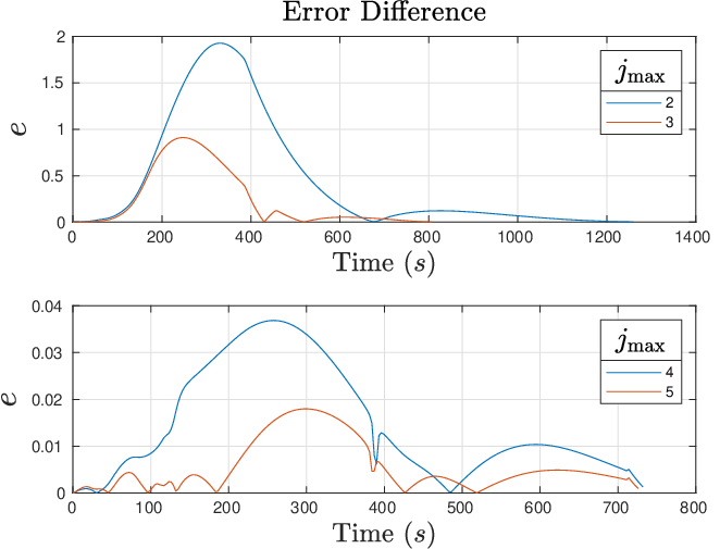
Furthermore, there is a trade-off between the value of $\mathchar 29034_{\max}$ and time it takes to reach $\mathchar 29048_{\mathchar 29028}$ . This is shown in Figure 3, where we plot the absolute difference between the time-constrained and optimal error. In addition, Figures 4 and 5 show that the attitudinal and translational states achieve the docking configuration given the initial conditions in Table 1 with $\mathchar 29034_{\max}\mathchar 12349\mathchar 28723$ . Figure 6 shows the positional trajectories in 3-D space achieving the docking configuration. A Monte Carlo simulation was performed with $\mathchar 29034_{\max}\mathchar 12349\mathchar 28723$ and the average error for $\mathchar 28725\mathchar 28720$ initial conditions was $\mathchar 28722\mathchar 314\mathchar 28726\mathchar 8705\mathchar 28721\mathchar 28720^{\mathchar 8704\mathchar 28723}$ . These results show that time-constrained MPC can control the deputy to the docking configuration using unperturbed states. Table 2 shows that we achieve at least a 23.98% reduction in average time to solve Problem 3 at each time $\mathchar 29035$ , for all values of $\mathchar 29034_{\max}$ that we used. Moreover, Table 2 shows a reduction of more than 92% in the maximum loop time for the worst case solving time for all $\mathchar 29034_{\max}$ . Next, we demonstrate the robustness of time-constrained MPC to perturbations.

Table 2: Solver times and reductions for Problem 3 without perturbations

$\mathchar 29034_{\max}$	Average Time/Loop Reduction (s)	Average Time/Loop Reduction (%)	Maximum Loop Time Reduction (s)	Maximum Loop Time Reduction (%)
2	0.5159	30.52%	26.40	95.59%
3	0.4245	25.11%	26.09	94.48%
4	0.4283	25.33%	25.75	93.26%
5	0.4054	23.98%	25.43	92.09%

4.3 Perturbed Results

One advantage of MPC is robustness to perturbations. In these simulations, at each time $\mathchar 29035$ , we add a disturbance $\mathchar 28961\delimiter 67273472\mathchar 29035\delimiter 84054785$ to the state $\mathchar 29048\delimiter 67273472\mathchar 29035\delimiter 84054785$ . The initial state for the next MPC loop, at time $\mathchar 29035\mathchar 8235\mathchar 28721$ was $\mathchar 29048\delimiter 67273472\mathchar 28720\delimiter 84054785\mathchar 12349\mathchar 29031_{\mathchar 29028}\delimiter 67273472\mathchar 29048\delimiter 67273472\mathchar 29035\delimiter 84054785\mathchar 24891\mathchar 29045\delimiter 67273472\mathchar 29035\delimiter 84054785\delimiter 84054785\mathchar 8235\mathchar 28961\delimiter 67273472\mathchar 29035\delimiter 84054785$ . The components of the perturbation vector $\mathchar 28961\delimiter 67273472\mathchar 29035\delimiter 84054785\mathchar 12850\mathbb{\mathchar 29010}^{\mathchar 28721\mathchar 28723}$ were sampled from multivariate normal distributions as

\mathchar 28961\delimiter 67273472\mathchar 29035\delimiter 84054785\mathchar 12824\begin{\mathchar29040\mathchar29037\mathchar29025\mathchar29044\mathchar29042\mathchar29033\mathchar29048}\mathchar 28721\mathchar 28720^{\mathchar 8704\mathchar 28723}\mathchar 8706\mathcal{\mathchar 29006}\delimiter 67273472\mathbf{\mathchar 28720}_{\mathchar 28723}\mathchar 24891\mathchar 29001_{\mathchar 28723}\delimiter 84054785\\ \mathchar 28721\mathchar 28720^{\mathchar 8704\mathchar 28726}\mathchar 8706\mathcal{\mathchar 29006}\delimiter 67273472\mathbf{\mathchar 28720}_{\mathchar 28723}\mathchar 24891\mathchar 29001_{\mathchar 28723}\delimiter 84054785\\ \mathchar 28721\mathchar 28720^{\mathchar 8704\mathchar 28728}\mathchar 8706\mathcal{\mathchar 29006}\delimiter 67273472\mathbf{\mathchar 28720}_{\mathchar 28724}\mathchar 24891\mathchar 29001_{\mathchar 28724}\delimiter 84054785\\ \mathchar 28721\mathchar 28720^{\mathchar 8704\mathchar 28726}\mathchar 8706\mathcal{\mathchar 29006}\delimiter 67273472\mathbf{\mathchar 28720}_{\mathchar 28723}\mathchar 24891\mathchar 29001_{\mathchar 28723}\delimiter 84054785\\ \end{\mathchar29040\mathchar29037\mathchar29025\mathchar29044\mathchar29042\mathchar29033\mathchar29048}\mathchar 314

(17)

We consider the same initial condition from Table 1 and same problem parameters from the previous subsection. In this subsection, we declare that we have achieved the docking configuration when $\delimiter 69645069\mathchar 29050\delimiter 67273472\mathchar 29035\delimiter 84054785\mathchar 8704\mathchar 29050_{\mathchar 29028}\delimiter 69645069_{\mathchar 561}\mathchar 12820\mathchar 28725\mathchar 8706\mathchar 28721\mathchar 28720^{\mathchar 8704\mathchar 28723}$ . Figure 7 shows that the deputy still achieves the docking configuration with the chief subject to perturbations and limited computational time. It takes more time to achieve the docking configuration for each $\mathchar 29034_{\max}$ compared to the unperturbed case (cf. Figure 2).

The optimal error trajectory takes longer to reach zero than the error trajectories generated under the computational time constraint. This differs from the unperturbed case and is perhaps counterintuitive, but is easily explained. The optimal error trajectory takes longer to reach zero because the control inputs are computed using our dynamic model without knowledge of the perturbations. Because future perturbations are unknown, exactly solving for an optimum while predicting future states does not necessarily give the best performance. In Figures 8 and 9 we show the states and inputs under perturbations for the initial conditions in Table 1 and $\mathchar 29034_{\max}\mathchar 12349\mathchar 28723$ .

These plots are similar to the unperturbed case but we can see the effect of perturbations, especially in the attitude error in Figure 8(a). In all cases, the docking configuration is successfully reached. Table 3 shows that we achieve at least a 23.98% reduction in average solving time per MPC loop for all values of $\mathchar 29034_{\max}$ . Table 3 also shows a roughly 95% reduction in the worst case solving time for all $\mathchar 29034_{\max}$ .

Table 3: Solver times and reductions for Problem 3 with perturbations

$\mathchar 29034_{\max}$	Average Time/Loop Reduction (s)	Average Time/Loop Reduction (%)	Maximum Loop Time Reduction (s)	Maximum Loop Time Reduction (%)
2	0.3616	36.16%	26.64	95.80%
3	0.2385	23.85%	26.33	94.70%
4	0.2029	20.29%	26.66	95.86%
5	0.2396	23.96%	26.65	95.86%

5 Conclusion

We proposed a time-constrained MPC control strategy for the 6 degree of freedom ARPOD problem, and showed that we can achieve the desired docking configuration under restrictive computational time constraints. Moreover, we demonstrated the robustness of docking using time-constrained MPC where the states of the system were subject to perturbations.

References

ESA (2022) (2022). Esa’s annual space environment report. Technical Report GEN-DB-LOG-00288-OPS-SD, ESA Space Debris Office, Darmstadt, Germany.
Bernhard et al. (2020) Bernhard, B., Choi, C., Rahmani, A., Chung, S.J., and Hadaegh, F. (2020). Coordinated motion planning for on-orbit satellite inspection using a swarm of small-spacecraft. In 2020 IEEE Aerospace Conference, 1–13.
Bourdarie and Xapsos (2008) Bourdarie, S. and Xapsos, M. (2008). The near-earth space radiation environment. IEEE transactions on nuclear science, 55(4), 1810–1832.
Cheng et al. (2018) Cheng, A.F., Rivkin, A.S., Michel, P., Atchison, J., Barnouin, O., Benner, L., Chabot, N.L., Ernst, C., Fahnestock, E.G., Kueppers, M., et al. (2018). Aida dart asteroid deflection test: Planetary defense and science objectives. Planetary and Space Science, 157, 104–115.
Curtis (2013) Curtis, H. (2013). Orbital mechanics for engineering students. Butterworth-Heinemann.
Di Cairano et al. (2012) Di Cairano, S., Park, H., and Kolmanovsky, I. (2012). Model predictive control approach for guidance of spacecraft rendezvous and proximity maneuvering. Int. J. of Robust and Nonlinear Control, 22(12), 1398–1427.
Dong et al. (2018) Dong, H., Hu, Q., and Akella, M. (2018). Dual-quaternion-based spacecraft autonomous rendezvous and docking under six-degree-of-freedom motion constraints. J. of Guidance, Control, and Dynamics, 41(5), 1150–1162.
Falcone et al. (2007) Falcone, P., Tufo, M., Borrelli, F., Asgari, J., and Tseng, H.E. (2007). A linear time varying model predictive control approach to the integrated vehicle dynamics control problem in autonomous systems. In 2007 46th IEEE Conference on Decision and Control, 2980–2985.
Graichen and Käpernick (2012) Graichen, K. and Käpernick, B. (2012). A real-time gradient method for nonlinear model predictive control. INTECH Open Access Publisher London.
Graichen and Kugi (2010) Graichen, K. and Kugi, A. (2010). Stability and incremental improvement of suboptimal mpc without terminal constraints. IEEE Trans. on Automatic Control, 55(11), 2576–2580.
Grüne and Pannek (2017) Grüne, L. and Pannek, J. (2017). Nonlinear model predictive control. In Nonlinear model predictive control, 45–69. Springer.
Hartley (2015) Hartley, E.N. (2015). A tutorial on model predictive control for spacecraft rendezvous. In 2015 European Control Conference (ECC), 1355–1361. IEEE.
Hartley and Maciejowski (2013) Hartley, E.N. and Maciejowski, J.M. (2013). Graphical fpga design for a predictive controller with application to spacecraft rendezvous. In 52nd IEEE Conference on Decision and Control, 1971–1976.
Hogan and Schaub (2014) Hogan, E.A. and Schaub, H. (2014). Attitude parameter inspired relative motion descriptions for relative orbital motion control. Journal of Guidance, Control, and Dynamics, 37(3), 741–749.
Hu et al. (2021) Hu, Q., Yang, H., Dong, H., and Zhao, X. (2021). Learning-based 6-dof control for autonomous proximity operations under motion constraints. IEEE Trans. on Aerospace and Electronic Systems, 57(6), 4097–4109.
Jewison (2017) Jewison, C.M. (2017). Guidance and Control for Multi-Stage Rendezvous and Docking Operations in the Presence of Uncertainty. Ph.D. thesis, Massachusetts Institute of Technology.
Kuipers (1999) Kuipers, J.B. (1999). Quaternions and rotation sequences: a primer with applications to orbits, aerospace, and virtual reality. Princeton university press.
Lee and Mesbahi (2017) Lee, U. and Mesbahi, M. (2017). Constrained autonomous precision landing via dual quaternions and model predictive control. Journal of Guidance, Control, and Dynamics, 40(2), 292–308.
Leomanni et al. (2014) Leomanni, M., Rogers, E., and Gabriel, S.B. (2014). Explicit model predictive control approach for low-thrust spacecraft proximity operations. Journal of Guidance, Control, and Dynamics, 37(6), 1780–1790.
Li et al. (2017) Li, Q., Yuan, J., Zhang, B., and Gao, C. (2017). Model predictive control for autonomous rendezvous and docking with a tumbling target. Aerospace Science and Technology, 69, 700–711.
Lovelly and George (2017) Lovelly, T.M. and George, A.D. (2017). Comparative analysis of present and future space-grade processors with device metrics. Journal of Aerospace Information Systems, 14(3), 184–197.
Lovelly (2017) Lovelly, T.M. (2017). Comparative Analysis of Space-Grade Processors. Ph.D. thesis, University of Florida.
Malyuta et al. (2021) Malyuta, D., Yu, Y., Elango, P., and Açıkmeşe, B. (2021). Advances in trajectory optimization for space vehicle control. Annual Reviews in Control, 52, 282–315.
Mayne (2014) Mayne, D.Q. (2014). Model predictive control: Recent developments and future promise. Automatica, 50(12), 2967–2986.
Ogilvie et al. (2008) Ogilvie, A., Allport, J., Hannah, M., and Lymer, J. (2008). Autonomous robotic operations for on-orbit satellite servicing. In Sensors and Systems for Space Applications II, volume 6958, 50–61.
Pavlov et al. (2019) Pavlov, A., Shames, I., and Manzie, C. (2019). Early termination of nmpc interior point solvers: Relating the duality gap to stability. In 2019 18th European Control Conference (ECC), 805–810. IEEE.
Petersen et al. (2014) Petersen, C., Jaunzemis, A., Baldwin, M., Holzinger, M., and Kolmanovsky, I. (2014). Model predictive control and extended command governor for improving robustness of relative motion guidance and control. In Proc. AAS/AIAA space flight mechanics meeting.
Richards and How (2003) Richards, A. and How, J.P. (2003). Model predictive control of vehicle maneuvers with guaranteed completion time and robust feasibility. In 2003 American Control Conference, volume 5, 4034–4040.
Soderlund and Phillips (2022) Soderlund, A.A. and Phillips, S. (2022). Autonomous rendezvous and proximity operations of an underactuated spacecraft via switching controls. In AIAA SCITECH 2022 Forum, 0956.
Soderlund et al. (2021) Soderlund, A.A., Phillips, S., Zaman, A., and Petersen, C.D. (2021). Autonomous satellite rendezvous and proximity operations via geometric control methods. In AIAA Scitech 2021 Forum, 0075.
Sun and Huo (2015) Sun, L. and Huo, W. (2015). 6-dof integrated adaptive backstepping control for spacecraft proximity operations. IEEE Transactions on Aerospace and Electronic Systems, 51(3), 2433–2443.
Trivailo et al. (2009) Trivailo, P.M., Wang, F., and Zhang, H. (2009). Optimal attitude control of an accompanying satellite rotating around the space station. Acta Astronautica, 64(2-3), 89–94.
Wächter and Biegler (2006) Wächter, A. and Biegler, L.T. (2006). On the implementation of an interior-point filter line-search algorithm for large-scale nonlinear programming. Mathematical programming, 106(1), 25–57.
Wang et al. (2018) Wang, X., Wang, Z., and Zhang, Y. (2018). Model predictive control to autonomously approach a failed spacecraft. Int. J. of Aerospace Engineering, 2018.
Wang and Ji (2019) Wang, Y. and Ji, H. (2019). Integrated relative position and attitude control for spacecraft rendezvous with iss and finite-time convergence. Aerospace Science and Technology, 85, 234–245.
Yang and Stoll (2019) Yang, J. and Stoll, E. (2019). Adaptive sliding mode control for spacecraft proximity operations based on dual quaternions. Journal of Guidance, Control, and Dynamics, 42(11), 2356–2368.
Zhou et al. (2020) Zhou, B.Z., Liu, X.F., and Cai, G.P. (2020). Motion-planning and pose-tracking based rendezvous and docking with a tumbling target. Advances in Space Research, 65(4), 1139–1157.