跳到论文正文
W Papers独立论文阅读器 arXiv:2211.11613 论文正文 计算阅读时间 · 0%
引用这篇论文根据当前论文元数据生成,正式投稿前建议核对。


License: CC BY 4.0
arXiv:2211.11613v2 [stat.CO] 24 Aug 2023

Improving multiple-try Metropolis with local balancing

Philippe Gagnon    Florian Maire    Giacomo Zanella
Abstract

Multiple-try Metropolis (MTM) is a popular Markov chain Monte Carlo method with the appealing feature of being amenable to parallel computing. At each iteration, it samples several candidates for the next state of the Markov chain and randomly selects one of them based on a weight function. The canonical weight function is proportional to the target density. We show both theoretically and empirically that this weight function induces pathological behaviours in high dimensions, especially during the convergence phase. We propose to instead use weight functions akin to the locally-balanced proposal distributions of Zanella 2020, thus yielding MTM algorithms that do not exhibit those pathological behaviours. To theoretically analyse these algorithms, we study the high-dimensional performance of ideal schemes that can be thought of as MTM algorithms which sample an infinite number of candidates at each iteration, as well as the discrepancy between such schemes and the MTM algorithms which sample a finite number of candidates. Our analysis unveils a strong distinction between the convergence and stationary phases: in the former, local balancing is crucial and effective to achieve fast convergence, while in the latter, the canonical and novel weight functions yield similar performance. Numerical experiments include an application in precision medicine involving a computationally-expensive forward model, which makes the use of parallel computing within MTM iterations beneficial.

1Department of Mathematics and Statistics, Université de Montréal, Canada.

2Department of Decision Sciences, BIDSA & IGIER, Bocconi University, Italy.

Keywords: Bayesian statistics; Markov chain Monte Carlo; parallel computing; random-walk Metropolis; scaling limit; weak convergence.

1 Introduction

1.1 Multiple-try Metropolis

In this paper, we study a specific Markov chain Monte Carlo (MCMC) method introduced by Liu et al. 2000 called Multiple-try Metropolis (MTM). It can be seen as a generalization of the Metropolis–Hastings (MH, Metropolis et al. 1953 and Hastings 1970) algorithm: at each iteration, several candidates for the next state of the Markov chain (instead of one) are sampled, hence the name of the algorithm. MTM can be used to sample from an intractable distribution π\pi for Monte Carlo integration purposes, where intractable here refers to the impossibility to compute integrals exactly with respect to that distribution. In a sampling context, such a distribution is called the target distribution. This distribution often is a posterior distribution of model parameters resulting from a Bayesian model. In the following, we assume for simplicity that π\pi admits a strictly positive probability density function (PDF) with respect to Lebesgue measure, implying that the model parameters in a Bayesian context are continuous random variables; to simplify the notation, we will also use π\pi to denote the PDF. When the latter is a posterior density, it is proportional to the product of the likelihood function and a prior density. Its normalizing constant is not available, but it is assumed here that the target density can be evaluated pointwise (up to that normalizing constant).

In its simplest and most popular form, an iteration of MTM is as follows11 1 We follow the formulation of Bédard et al. 2012.:

  1. 1.

    NN values 𝐲1,…,𝐲N∈ℝd\mathbf{y}_{1},\ldots,\mathbf{y}_{N}\in\R^{d} are sampled independently from a proposal distribution with density qσ​(𝐱,⋅)q_{\sigma}(\mathbf{x},\cdot\,), where 𝐱∈ℝd\mathbf{x}\in\R^{d} is the current state of the chain and σ>0\sigma>0 is a fixed scale parameter;

  2. 2.

    one of the 𝐲i\mathbf{y}_{i}’s is randomly selected to be the proposal for the next state of the chain, say 𝐲j\mathbf{y}_{j}, with probability proportional to a weight w⁡(𝐱,𝐲j)w(\mathbf{x},\mathbf{y}_{j}), where ww is a strictly positive weight function;

  3. 3.

    N−1N-1 values 𝐳1,…,𝐳N−1\mathbf{z}_{1},\ldots,\mathbf{z}_{N-1} are sampled independently from qσ​(𝐲j,⋅)q_{\sigma}(\mathbf{y}_{j},\cdot\,);

  4. 4.

    the proposal is accepted, meaning that the next state is set to be 𝐲j\mathbf{y}_{j}, with probability

    α⁡(𝐱,𝐲j):=1∧π⁡(𝐲j)​qσ​(𝐲j,𝐱)​w​(𝐲j,𝐱)/(∑i=1N−1w⁡(𝐲j,𝐳i)+w⁡(𝐲j,𝐱))π⁡(𝐱)​qσ​(𝐱,𝐲j)​w​(𝐱,𝐲j)/(∑i=1Nw⁡(𝐱,𝐲i)),\displaystyle\alpha(\mathbf{x},\mathbf{y}_{j}):=1\wedge\frac{\pi(\mathbf{y}_{j})\,q_{\sigma}(\mathbf{y}_{j},\mathbf{x})\,w(\mathbf{y}_{j},\mathbf{x})\bigg/\left(\sum_{i=1}^{N-1}w(\mathbf{y}_{j},\mathbf{z}_{i})+w(\mathbf{y}_{j},\mathbf{x})\right)}{\pi(\mathbf{x})\,q_{\sigma}(\mathbf{x},\mathbf{y}_{j})\,w(\mathbf{x},\mathbf{y}_{j})\bigg/\left(\sum_{i=1}^{N}w(\mathbf{x},\mathbf{y}_{i})\right)}, (1)

    where a∧b:=min⁡(a,b)a\wedge b:=\min(a,b) and the dependence of α⁡(𝐱,𝐲j)\alpha(\mathbf{x},\mathbf{y}_{j}) on 𝐲i,i≠j\mathbf{y}_{i},i\neq j, and 𝐳1,…,𝐳N−1\mathbf{z}_{1},\ldots,\mathbf{z}_{N-1} is made implicit to simplify the notation; when the proposal is rejected the chain remains at 𝐱\mathbf{x}.

Step 3 and the specific form of the acceptance probability (1) are crucial ingredients to make the resulting Markov chains reversible with respect to π\pi and thus to ensure that π\pi is an invariant distribution and the algorithm is valid (see Liu et al. 2000 for full details). Typically, in Step 1, the sampling is performed through a random-walk scheme, and in particular, using a normal with a mean 𝐱\mathbf{x} and a diagonal covariance matrix with diagonal elements given by σ2\sigma^{2}, denoted by qσ​(𝐱,⋅)=𝒩⁡(𝐱,σ2​𝕀d)q_{\sigma}(\mathbf{x},\cdot\,)=\mathcal{N}(\mathbf{x},\sigma^{2}\mathbb{I}_{d}), with 𝕀d\mathbb{I}_{d} being the identity matrix of size dd (we also use qσ​(𝐱,⋅)q_{\sigma}(\mathbf{x},\cdot\,) to denote the distribution to simplify). Note that the terms qσ​(𝐲j,𝐱)q_{\sigma}(\mathbf{y}_{j},\mathbf{x}) and qσ​(𝐱,𝐲j)q_{\sigma}(\mathbf{x},\mathbf{y}_{j}) in (1) cancel each other when the density is symmetric as with the normal. In Steps 2 and 4, the weight function w⁡(𝐱,𝐲)w(\mathbf{x},\mathbf{y}) is typically a function of the ratio π⁡(𝐲)/π⁡(𝐱)\pi(\mathbf{y})/\pi(\mathbf{x}), the most popular choice by far being w⁡(𝐱,𝐲)=π⁡(𝐲)/π⁡(𝐱)∝π⁡(𝐲)w(\mathbf{x},\mathbf{y})=\pi(\mathbf{y})/\pi(\mathbf{x})\propto\pi(\mathbf{y}). Randomly choosing among the candidates 𝐲1,…,𝐲N\mathbf{y}_{1},\ldots,\mathbf{y}_{N} based on a function of their target-density evaluations π⁡(𝐲1),…,π⁡(𝐲N)\pi(\mathbf{y}_{1}),\ldots,\pi(\mathbf{y}_{N}) makes MTM an informed scheme, in the sense of Zanella 2020, meaning that it leverages target-distribution information in the proposal mechanism. Such schemes can improve in terms of asymptotic variance of ergodic averages and mixing properties over their uninformed counterparts.

1.2 Potential of MTM and parallel computing in MCMC

MTM is appealing in situations where it is computationally expensive to evaluate the target density (typically because of the likelihood function), and it is not possible to obtain an explicit form of its gradient. In this situation, gradient-based MCMC methods may be either inapplicable or computationally intensive, e.g., if repeated numerical derivative approximations are required. Practitioners facing such a situation may naturally consider using a MH sampler with a random-walk proposal mechanism qσq_{\sigma}, or its MTM generalization.22 2 One could also use MTM with an informed gradient-based proposal distribution, but this is less common in practice. The weights in Steps 2 and 4 in MTM can be computed in parallel, which results in a significant computation-time reduction compared to serial computation when the iteration cost is largely dominated by that of evaluating the target density. In this situation, the iteration cost of MTM is roughly twice that of a MH sampler using the proposal distribution qσq_{\sigma}.33 3 When the iteration cost is largely dominated by that of evaluating the target density, we know that the computational cost of the other operations (like sampling from qσ​(𝐱,⋅)q_{\sigma}(\mathbf{x},\cdot\,)) is negligible compared with that of evaluating the target density. This implies that the iteration cost of the MH sampler roughly corresponds to that of evaluating the target density once for evaluating the acceptance probability (π⁡(𝐱)\pi(\mathbf{x}) can have been recorded from the previous iteration), and the iteration cost of MTM roughly corresponds to that of evaluating the target density twice (because the weights in Steps 2 and 4 in MTM can be computed in parallel).

We refer to the type of parallelization employed in MTM as in-step parallelization, given that parallel computing is used within each algorithm iteration. It is to be contrasted with a basic use of parallel computing where one runs NN MH algorithms in parallel each using the proposal distribution qσq_{\sigma}. The advantage of the latter is that it is an embarrassingly parallel workload with essentially no communication cost (see, e.g., Rosenthal 2000 and Jacob et al. 2020). It however does not reduce the burn-in required by each chain to reach stationarity, and thus its computational speed-up compared to running one MH algorithm is fundamentally limited if the chains have a large mixing time. As a result, in-step parallelization approaches that reduce burn-in can lead to significant gain in efficiency in the convergence phase; see, e.g., discussions in Neal 2003, Tjelmeland 2004, Frenkel 2004, Calderhead 2014 and Holbrook 2023.

In order to reduce the burn-in significantly enough to gain in efficiency with MTM, one has to choose carefully the weight function ww. As mentioned, the most popular weight function is w⁡(𝐱,𝐲)=π⁡(𝐲)/π⁡(𝐱)∝π⁡(𝐲)w(\mathbf{x},\mathbf{y})=\pi(\mathbf{y})/\pi(\mathbf{x})\propto\pi(\mathbf{y}). The intuition behind choosing this weight function is to select 𝐲j\mathbf{y}_{j} among the candidates 𝐲1,…,𝐲N\mathbf{y}_{1},\ldots,\mathbf{y}_{N} proportionally to its “probability” under the target. Although intuitively sensible, this choice lacks theoretical justification and, in fact, has been observed to yield an MTM algorithm with pathological behaviours. For example, Martino and Louzada 2017 highlights that MTM with w⁡(𝐱,𝐲)∝π⁡(𝐲)w(\mathbf{x},\mathbf{y})\propto\pi(\mathbf{y}) may have issues of convergence if initialized in the tails of the target density because of acceptance probabilities that are near zero in this area, resulting in Markov chains that get stuck. Also, performance often decreases as NN increases, which is counter-intuitive as the algorithm has a larger group of candidates to select the proposal from at each iteration. In this paper, we show that the cause of those issues is precisely the choice of weight function w⁡(𝐱,𝐲)∝π⁡(𝐲)w(\mathbf{x},\mathbf{y})\propto\pi(\mathbf{y}) which makes the resulting MTM globally balanced, a qualifier coined by Zanella 2020 and that will be justified. Note that alternative choices are discussed in, e.g., Liu et al. 2000 and Pandolfi et al. 2010, but these are similar in spirit to the choice w⁡(𝐱,𝐲)∝π⁡(𝐲)w(\mathbf{x},\mathbf{y})\propto\pi(\mathbf{y}) and are exposed to the same pathologies.

The global objective of this work is to identify effective weight functions based on theoretical arguments and to study the resulting MTM algorithms. The effective weight functions that we identify, such as w⁡(𝐱,𝐲)∝π⁡(𝐲)w(\mathbf{x},\mathbf{y})\propto\sqrt{\pi(\mathbf{y})}, yield MTM algorithms that have a connection with the locally-balanced samplers proposed by Zanella 2020 in the context of discrete state-spaces. Therein, a large class of informed samplers are studied, with proposal distributions resulting from a combination of a random-walk proposal scheme and what is referred to as a balancing function. A specific choice of balancing function makes the sampler locally balanced. As already noted in Zanella 2020, the weight function in MTM and the balancing function play an analogous role. Given the domination of the locally-balanced sampler over the globally-balanced one shown in Zanella 2020, it is thus natural to consider the use of locally-balanced weight functions in MTM, especially given that the resulting samplers have the same computational cost as their globally-balanced counterpart and are as easy to implement. In this paper, we refer to MTM with the weight function w⁡(𝐱,𝐲)=π⁡(𝐲)/π⁡(𝐱)w(\mathbf{x},\mathbf{y})=\pi(\mathbf{y})/\pi(\mathbf{x}) as globally-balanced (GB) MTM and to MTM with a locally-balanced weight function as locally-balanced (LB) MTM. It will be highlighted in the following that LB MTM is closely related to gradient-based MCMC methods such as the Metropolis-adjusted Langevin algorithm (MALA, Roberts and Tweedie 1996) and the Barker proposal scheme of Livingstone and Zanella 2022.

1.3 Organization of the paper

We now describe how the rest of the paper is organized. In Section 2, we establish a weak convergence of the Markov chains simulated by MTM towards those simulated by an ideal sampling scheme, as N→∞N\rightarrow\infty with the dimension dd fixed. This ideal sampling scheme is the continuous state-space counterpart of the class of informed samplers studied in Zanella 2020. In Section 3, we study the convergence phase of MTM algorithms through both theoretical and empirical results. The analysis shows that GB MTM indeed often has issues of convergence, while LB MTM does not. In fact, LB MTM provides drastic convergence speed-ups and improved robustness compared to GB MTM. In Section 4, we study MTM properties in stationarity. Theorem 2 provides high-dimensional scaling-limit results (as d→∞d\rightarrow\infty) for the ideal scheme with w⁡(𝐱,𝐲)∝π⁡(𝐲)w(\mathbf{x},\mathbf{y})\propto\pi(\mathbf{y}) and that with a LB weight function, namely w⁡(𝐱,𝐲)∝π⁡(𝐲)w(\mathbf{x},\mathbf{y})\propto\sqrt{\pi(\mathbf{y})}. Theorem 3 then shows that these ideal schemes are approached by MTM under conditions on the rate at which the number of candidates increases with the dimension. Combining Theorems 2 and 3 leads to an informative but somewhat negative conclusion: the ideal scheme with the LB weight function scales better with dimension, however, the (sufficient) condition under which the corresponding MTM algorithm reaches its full potential by approaching the ideal scheme is that NN scales exponentially with the dimension. As a result, in common situations, LB MTM provides only mild performance improvement compared to GB MTM in stationarity. The theoretical results of Sections 3 and 4 are derived in simple scenarios and numerical results are provided to illustrate them, including adaptive MTM implementations. To explore whether the scope of those theoretical results extends beyond simple scenarios, we study in Section 5 the application of GB and LB MTM to a real-world inference problem of immunotherapy in precision medicine where the likelihood is expensive to compute and its gradient is not available in closed form. The empirical results are consistent with the theoretical ones, including observing a drastically reduced burn-in time for LB MTM. We finish the manuscript with a discussion in Section 6. The proofs of all theoretical results are deferred to Appendix A. The code to reproduce all numerical results is available online.44 4 See ancillary files on arXiv:2211.11613.

While working on our manuscript, it came to our attention that Chang et al. 2022 independently and concurrently propose to use LB weight functions within MTM and study the resulting samplers, but the context and focus are quite different. The context and focus are that of sampling from target distributions defined on discrete state-spaces and more precisely from target distributions resulting from model-selection problems. Our contributions and theirs thus have virtually no overlap. That being said, the conclusions in Chang et al. 2022 and ours are consistent, and in this sense, the two studies are complementary.

2 Ideal schemes and locally-balanced weight functions

We start in Section 2.1 with the identification of LB weight functions as effective weight functions. The arguments motivating the use of such weight functions rest upon a theoretical result for which a sketch of a proof was presented in Liu et al. 2000. The result is stated informally in Section 2.1, while a formal statement is presented in Section 2.2. In Section 2.3, a connection between LB MTM and gradient-based methods is highlighted.

2.1 Locally-balanced weight functions: A motivation

Liu et al. 2000 presented a sketch of a proof of the convergence of the Markov kernel of MTM as N→∞N\rightarrow\infty to that of a MH algorithm using a proposal distribution with a PDF defined as

Qw,σ​(𝐱,𝐲):=w⁡(𝐱,𝐲)​qσ​(𝐱,𝐲)∫w⁡(𝐱,𝐲)​qσ​(𝐱,𝐲)​𝑑𝐲,\displaystyle Q_{w,\sigma}(\mathbf{x},\mathbf{y}):=\frac{w(\mathbf{x},\mathbf{y})\,q_{\sigma}(\mathbf{x},\mathbf{y})}{\int w(\mathbf{x},\mathbf{y})\,q_{\sigma}(\mathbf{x},\mathbf{y})\,\mathrm{d}\mathbf{y}},

assuming that the integral in the denominator exists and is finite. We will refer to the MH algorithm using the proposal distribution Qw,σQ_{w,\sigma} as an ideal scheme as it cannot in general be implemented and it can be thought of as an MTM algorithm sampling an infinite number of candidates NN at each iteration.55 5 For consistency, we will use the terminology “ideal scheme” also for the globally-balanced version even if using a large number of candidates NN is not effective in that case.

Whenever there exists a positive continuous function gg such that w⁡(𝐱,𝐲)w(\mathbf{x},\mathbf{y}) is of the form w⁡(𝐱,𝐲)=g⁡(π⁡(𝐲)/π⁡(𝐱))w(\mathbf{x},\mathbf{y})=g(\pi(\mathbf{y})/\pi(\mathbf{x})), the ideal scheme corresponds to the continuous version of the class of informed samplers studied in Zanella 2020. All the weight functions considered in our paper are of this form. Even though the work of Zanella 2020 is in the context of discrete state-spaces, a part of the analysis conducted therein is applicable to the continuous case as well. In particular, it indicates that the choice w⁡(𝐱,𝐲)∝π⁡(𝐲)w(\mathbf{x},\mathbf{y})\propto\pi(\mathbf{y}) yields a proposal distribution which leaves the target distribution invariant (without the MH correction) in the situation where σ→∞\sigma\rightarrow\infty, the approach being, in that sense, global; in fact, the limiting case corresponds to independent sampling. This justifies the fact that, MTM using the weight function w⁡(𝐱,𝐲)∝π⁡(𝐲)w(\mathbf{x},\mathbf{y})\propto\pi(\mathbf{y}) is coined globally-balanced (GB) MTM. Analogously, the ideal scheme using the proposal PDF Qw,σ​(𝐱,𝐲)∝π⁡(𝐲)​qσ​(𝐱,𝐲)Q_{w,\sigma}(\mathbf{x},\mathbf{y})\propto\pi(\mathbf{y})\,q_{\sigma}(\mathbf{x},\mathbf{y}) will be referred to as the globally-balanced (GB) ideal scheme.

The problem with using such a function ww is that, in high dimensions, the scale parameter of typical MCMC algorithms is required to be small to avoid near-zero acceptance probabilities, as indicated by the optimal-scaling theory (see, e.g., Bédard et al. 2012 in the specific context of MTM). As σ→0\sigma\rightarrow 0, using Qw,σ​(𝐱,𝐲)∝π⁡(𝐲)​qσ​(𝐱,𝐲)Q_{w,\sigma}(\mathbf{x},\mathbf{y})\propto\pi(\mathbf{y})\,q_{\sigma}(\mathbf{x},\mathbf{y}) leaves π2\pi^{2} invariant (without the MH correction), instead of π\pi. In high dimensions, when σ\sigma is small, there is thus a significant discrepancy between the proposal and target distributions, and this causes the pathological behaviours of GB MTM mentioned previously.

Locally-balanced (LB) proposal distributions aim at correcting this discrepancy. Indeed, by construction, LB proposal distributions leave π\pi invariant (without the MH correction) in the limiting situation where σ→0\sigma\rightarrow 0, which is the regime in agreement with high-dimensional settings. In our context, within ideal schemes, LB proposal distributions are such that Qw,σ​(𝐱,𝐲)∝g⁡(π⁡(𝐲)/π⁡(𝐱))​qσ​(𝐱,𝐲)Q_{w,\sigma}(\mathbf{x},\mathbf{y})\propto g(\pi(\mathbf{y})/\pi(\mathbf{x}))\,q_{\sigma}(\mathbf{x},\mathbf{y}), where the balancing function gg is a positive continuous function such that g⁡(x)/g⁡(1/x)=xg(x)/g(1/x)=x for x>0x>0. We thus propose to set the weight function in MTM to w⁡(𝐱,𝐲)=g⁡(π⁡(𝐲)/π⁡(𝐱))w(\mathbf{x},\mathbf{y})=g(\pi(\mathbf{y})/\pi(\mathbf{x})) with gg satisfying these conditions. Several functions gg satisfy these conditions (see, e.g., Zanella 2020, Sansone 2022 and Vogrinc et al. 2023). In this paper, we focus on two of them which have been thoroughly studied in other contexts (Power and Goldman 2019; Gagnon and Maire 2020; Gagnon 2021; Sun et al. 2021; Hird et al. 2022; Liang et al. 2022; Livingstone and Zanella 2022; Sun et al. 2022b; Sun et al. 2022a; Zhou and Smith 2022), namely g⁡(x)=xg(x)=\sqrt{x} and g⁡(x)=x/(1+x)g(x)=x/(1+x), the latter yielding what is called the Barker proposal distribution in reference to Barker 1965’s acceptance-probability choice. The ideal scheme using the proposal PDF Qw,σ​(𝐱,𝐲)∝g⁡(π⁡(𝐲)/π⁡(𝐱))​qσ​(𝐱,𝐲)Q_{w,\sigma}(\mathbf{x},\mathbf{y})\propto g(\pi(\mathbf{y})/\pi(\mathbf{x}))\,q_{\sigma}(\mathbf{x},\mathbf{y}) with gg satisfying the conditions above will thus be referred to as the locally-balanced (LB) ideal scheme. This justifies the fact that, MTM using the weight function w⁡(𝐱,𝐲)∝g⁡(π⁡(𝐲)/π⁡(𝐱))w(\mathbf{x},\mathbf{y})\propto g(\pi(\mathbf{y})/\pi(\mathbf{x})) with gg satisfying the conditions above is coined locally-balanced (LB) MTM.

LB MTM will be seen to not exhibit the pathological behaviours mentioned previously. Also, LB MTM with g⁡(x)=xg(x)=\sqrt{x} will be seen to have an advantage over that with the Barker weight function in terms of convergence speed-ups. This advantage has been observed in other contexts (Zhou and Smith 2022). Significant convergence speed-ups with g⁡(x)=xg(x)=\sqrt{x} have also been observed for MTM in Chang et al. 2022. In stationarity, the performance of LB MTM with g⁡(x)=xg(x)=\sqrt{x} is similar to that with the Barker weight function. All that suggests the following practical recommendation to MTM users: use LB weight functions, and more specifically, g⁡(x)=xg(x)=\sqrt{x}.

2.2 Convergence towards ideal schemes

To understand why the convergence of MTM towards the ideal scheme might hold, it is useful to have a characterization of the distribution of a proposal sampled using MTM, that we denote by 𝐘J\mathbf{Y}_{J} with a capital JJ to represent that the choice among the candidates for the proposal is random. This distribution is conditional on the current state of the Markov chain 𝐱\mathbf{x}, and we use 𝔼𝐱\mathbb{E}_{\mathbf{x}} to denote an expectation with respect to the associated PDF that depends on 𝐱\mathbf{x}. The PDF is based on the product measure ∏i=1Nqσ(𝐱,𝐲i)d𝐲1:N\prod_{i=1}^{N}q_{\sigma}(\mathbf{x},\mathbf{y}_{i})\,\mathrm{d}\mathbf{y}_{1:N}, where 𝐲1:N:=(𝐲1,…,𝐲N)\mathbf{y}_{1:N}:=(\mathbf{y}_{1},\ldots,\mathbf{y}_{N}). That characterization uses that 𝐘1,…,𝐘N\mathbf{Y}_{1},\ldots,\mathbf{Y}_{N} are conditionally independent and identically distributed (IID) given 𝐱\mathbf{x}.

Proposition 1.

Given a current state 𝐱\mathbf{x} and function hh, a proposal 𝐘J\mathbf{Y}_{J} sampled using MTM is such that

𝔼𝐱​[h​(𝐘J)]\displaystyle\mathbb{E}_{\mathbf{x}}[h(\mathbf{Y}_{J})] =∫h(𝐲1)w⁡(𝐱,𝐲1)1N​∑i=1Nw⁡(𝐱,𝐲i)∏i=1Nqσ(𝐱,𝐲i)d𝐲1:N.\displaystyle=\int h(\mathbf{y}_{1})\,\frac{w(\mathbf{x},\mathbf{y}_{1})}{\frac{1}{N}\sum_{i=1}^{N}w(\mathbf{x},\mathbf{y}_{i})}\prod_{i=1}^{N}q_{\sigma}(\mathbf{x},\mathbf{y}_{i})\,\mathrm{d}\mathbf{y}_{1:N}.

The expectation in Proposition 1 is to be compared with that of h⁡(𝐘)h(\mathbf{Y}) with 𝐘∼Qw,σ​(𝐱,⋅)\mathbf{Y}\sim Q_{w,\sigma}(\mathbf{x},\cdot\,), given a current state 𝐱\mathbf{x}, that can be written as

𝔼𝐱​[h​(𝐘)]\displaystyle\mathbb{E}_{\mathbf{x}}[h(\mathbf{Y})] =∫h(𝐲1)w⁡(𝐱,𝐲1)∫w⁡(𝐱,𝐲1)​qσ​(𝐱,𝐲1)​d​𝐲1∏i=1Nqσ(𝐱,𝐲i)d𝐲1:N.\displaystyle=\int h(\mathbf{y}_{1})\,\frac{w(\mathbf{x},\mathbf{y}_{1})}{\int w(\mathbf{x},\mathbf{y}_{1})\,q_{\sigma}(\mathbf{x},\mathbf{y}_{1})\,\mathrm{d}\mathbf{y}_{1}}\prod_{i=1}^{N}q_{\sigma}(\mathbf{x},\mathbf{y}_{i})\,\mathrm{d}\mathbf{y}_{1:N}. (2)

It is apparent that the expectation in Proposition 1 is an approximation that in (2) (and that one sampling scheme approximates the other), and that, presumably, the approximation becomes more accurate as NN increases.

We now present a formal result about the weak convergence of Markov chains simulated by MTM towards those simulated by the ideal sampling scheme, under some conditions. Let us denote a Markov chain simulated by MTM as {𝐗N​(m):m∈ℕ}\{\mathbf{X}_{N}(m):m\in\N\} and that simulated by the corresponding ideal algorithm by {𝐗ideal​(m):m∈ℕ}\{\mathbf{X}_{\text{ideal}}(m):m\in\N\}. Also, let us denote the Euclidean norm of a vector 𝐱\mathbf{x} by ‖𝐱‖\|\mathbf{x}\|.

Theorem 1.

Assume that 𝔼⁡[w​(𝐗,𝐘1)4]<∞\mathbb{E}[w(\mathbf{X},\mathbf{Y}_{1})^{4}]<\infty and 𝔼⁡[w​(𝐗,𝐘1)−4]<∞\mathbb{E}[w(\mathbf{X},\mathbf{Y}_{1})^{-4}]<\infty with 𝐗∼π\mathbf{X}\sim\pi and 𝐘1|𝐗∼qσ​(𝐗,⋅)\mathbf{Y}_{1}\mid\mathbf{X}\sim q_{\sigma}(\mathbf{X},\cdot\,). As N→∞N\rightarrow\infty,

  1. 1.

    given any state 𝐱\mathbf{x}, the total variation between the distribution of a proposal 𝐘J\mathbf{Y}_{J} sampled using MTM and Qw,σ​(𝐱,⋅)Q_{w,\sigma}(\mathbf{x},\cdot\,) converges to 0 at a rate of 1/N1/\sqrt{N};

  2. 2.

    if additionally

    (a)

    π\pi, Qw,σ​(⋅,𝐲)Q_{w,\sigma}(\,\cdot\,,\mathbf{y}) and Qw,σ​(𝐲,⋅)Q_{w,\sigma}(\mathbf{y},\cdot\,) are continuous, for any 𝐲\mathbf{y},

    (b)

    for all 𝐱∈ℝd\mathbf{x}\in\R^{d}, there exists an ε>0\varepsilon>0 and an integrable function f⁡(𝐱,⋅)f(\mathbf{x},\cdot\,) such that

    sup{ϵ∈ℝd:‖ϵ‖≤ε}Qw,σ(𝐱+ϵ,𝐲)≤f(𝐱,𝐲),\sup_{\{\boldsymbol{\epsilon}\in\R^{d}:\|\boldsymbol{\epsilon}\|\leq\varepsilon\}}Q_{w,\sigma}(\mathbf{x}+\boldsymbol{\epsilon},\mathbf{y})\leq f(\mathbf{x},\mathbf{y}),

    for all 𝐲∈ℝd\mathbf{y}\in\R^{d},

    then {𝐗N​(m):m∈ℕ}\{\mathbf{X}_{N}(m):m\in\N\} converges weakly towards {𝐗ideal​(m):m∈ℕ}\{\mathbf{X}_{\text{ideal}}(m):m\in\N\} provided that 𝐗N​(0)∼π\mathbf{X}_{N}(0)\sim\pi and 𝐗ideal​(0)∼π\mathbf{X}_{\text{ideal}}(0)\sim\pi.

This result indicates that MTM can be seen as an approximation to the ideal MH scheme using Qw,σQ_{w,\sigma} as a proposal distribution. The latter will thus be considered instead of the former for theoretical analyses in the next sections. The advantage of doing so is that the ideal scheme samples only one candidate at each iteration and is thus easier to analyse. A refined version of Theorem 1 will be provided in Section 4.2; it allows to quantitatively evaluate the discrepancy between the chains simulated by MTM and the ideal scheme.

We finish this section with a result indicating that Assumption (b) in part 2 of Theorem 1 is verified in great generality.

Proposition 2.

Assume that π\pi is upper bounded, qσ​(𝐱,⋅)=𝒩⁡(𝐱,σ2​𝕀d)q_{\sigma}(\mathbf{x},\cdot\,)=\mathcal{N}(\mathbf{x},\sigma^{2}\mathbb{I}_{d}), and w⁡(𝐱,𝐲)=π⁡(𝐲)/π⁡(𝐱)w(\mathbf{x},\mathbf{y})=\pi(\mathbf{y})/\pi(\mathbf{x}) or w⁡(𝐱,𝐲)=π⁡(𝐲)/π⁡(𝐱)w(\mathbf{x},\mathbf{y})=\sqrt{\pi(\mathbf{y})/\pi(\mathbf{x})}. Then, Assumption (b) in part 2 of Theorem 1 is satisfied.

2.3 Locally-balanced MTM as a gradient-free alternative

An indirect connection can be established between MTM using g⁡(x)=xg(x)=\sqrt{x} and MALA, and between MTM using g⁡(x)=x/(1+x)g(x)=x/(1+x) and the MH sampler based on the Barker proposal scheme of Livingstone and Zanella 2022. Recall that both MALA and the Barker scheme are gradient-based MCMC algorithms which require that π\pi is differentiable and that ∇log⁡π\nabla\log\pi can be evaluated pointwise. Interestingly, the MALA proposal can be viewed as an approximation to the ideal scheme using g⁡(x)=xg(x)=\sqrt{x}, whereas the Barker proposal can be viewed as an approximation to that using g⁡(x)=x/(1+x)g(x)=x/(1+x). Indeed, they both result from an approximation of Qw,σ​(𝐱,⋅)Q_{w,\sigma}(\mathbf{x},\cdot\,) based on a first-order Taylor series expansion of log⁡π\log\pi:

Qw,σ​(𝐱,𝐲)∝g⁡(elog⁡π⁡(𝐲)−log⁡π⁡(𝐱))​qσ​(𝐱,𝐲)≈g⁡(e(∇log⁡π​(𝐱))T​(𝐲−𝐱))​qσ​(𝐱,𝐲).Q_{w,\sigma}(\mathbf{x},\mathbf{y}\,)\propto g(\mathrm{e}^{\log\pi(\mathbf{y})-\log\pi(\mathbf{x})})\,q_{\sigma}(\mathbf{x},\mathbf{y})\approx g(\mathrm{e}^{(\nabla\log\pi(\mathbf{x}))^{T}(\mathbf{y}-\mathbf{x})})\,q_{\sigma}(\mathbf{x},\mathbf{y}).

When g⁡(x)=xg(x)=\sqrt{x} and qσ​(𝐱,⋅)=𝒩⁡(𝐱,σ2​𝕀d)q_{\sigma}(\mathbf{x},\cdot\,)=\mathcal{N}(\mathbf{x},\sigma^{2}\mathbb{I}_{d}), normalizing the last expression gives exactly the MALA proposal, while, when g⁡(x)=x/(1+x)g(x)=x/(1+x), it gives the Barker scheme (see, respectively, Section 5 of Zanella 2020 and Section 3 of Livingstone and Zanella 2022). Thus, we can see MALA and the Barker proposal scheme as gradient-based approximations of the same ideal schemes as those approximated by LB MTM samplers with g⁡(x)=xg(x)=\sqrt{x} and g⁡(x)=x/(1+x)g(x)=x/(1+x). The approximations used in MTM are different in several aspects. First, they are stochastic, by opposition to deterministic as in the gradient-based methods. Second, one has control over the approximations (through NN). Last but not least, the algorithms do not require to evaluate the gradient of log⁡π\log\pi, which is advantageous when evaluating the gradient is either infeasible or computationally intensive.

GB MTM approximates an ideal scheme which does not correspond to any known first-order method. A rich body of literature has shown that MALA and the MH sampler with the Barker scheme behave quantitatively and qualitatively differently (in terms of ergodicity measure or scaling-limit regime) to most zero-th order methods such as random-walk Metropolis (see, e.g., Roberts and Rosenthal 1998, Bou-Rabee and Hairer 2013, Dwivedi et al. 2018 and Livingstone and Zanella 2022). It is thus important to study whether LB MTM inherits some of those favourable properties, which cannot be expected by GB MTM.

3 Performance during the convergence phase

In this section, we evaluate the performance during the convergence phase66 6 By convergence phase, often called burn-in in the MCMC literature, we mean the iterations until the Markov chain simulated by MTM is close in distribution to π\pi. of MTM with the different weight functions. We do this by analysing the acceptance probabilities in the tails in Section 3.1 and by empirically measuring the convergence time of adaptively tuned MTM in Section 3.2. The adaptive tuning aims to represent how one would use and tune MTM in practice. As mentioned previously, the acceptance probabilities are near-zero in the tails with GB MTM, unless the step size σ\sigma is made extremely small, which causes convergence issues in either case. Our analysis shows that these convergence issues do not arise with LB MTM. Also, numerical results show that MTM with the Barker weight function has higher acceptance probabilities than that with g⁡(x)=xg(x)=\sqrt{x}. This advantage has been observed in other contexts (Zanella 2020; Livingstone and Zanella 2022), and is attributed to the boundedness of the function g⁡(x)=x/(1+x)g(x)=x/(1+x). In the MTM context, it yields more stability in the approximation of the ideal scheme. Even though the unboundedness of g⁡(x)=xg(x)=\sqrt{x} yields less stability, it leads to more persistent movement from the tails to the high-probability region, which is shown in Section 3.2 to provide better convergence performance.

3.1 Acceptance probabilities in the tails

In this section, we analyse the behaviour of MTM when initialized in the tails by evaluating the conditional expected acceptance probability, given an initial state 𝐱\mathbf{x} with ‖𝐱‖\|\mathbf{x}\| large, where the expectation is with respect to the random variables involved in the proposal mechanism. A low conditional expected acceptance probability implies that it is likely that the chain gets stuck and that an issue arises in terms of convergence to the target distribution as the algorithm progresses. The analysis rests upon a theoretical result about the ideal scheme. The result is established under a specific and simple scenario: the target density factorizes, and more precisely,

π⁡(𝐱)=∏i=1dφ⁡(xi),𝐱:=(x1,…,xd)T∈ℝd,\displaystyle\pi(\mathbf{x})=\prod_{i=1}^{d}\varphi(x_{i}),\quad\mathbf{x}:=(x_{1},\ldots,x_{d})^{T}\in\R^{d}, (3)

and qσ​(𝐱,⋅)=𝒩⁡(𝐱,σ2​𝕀d)q_{\sigma}(\mathbf{x},\cdot\,)=\mathcal{N}(\mathbf{x},\sigma^{2}\mathbb{I}_{d}), where φ\varphi is the PDF of a standard normal distribution. The normal assumption and the factorization allow to make precise calculations and in particular to establish that Qw,σQ_{w,\sigma} is a normal distribution when the weight function factorizes as well, that is when using for instance w⁡(𝐱,𝐲)=π⁡(𝐲)/π⁡(𝐱)w(\mathbf{x},\mathbf{y})=\pi(\mathbf{y})/\pi(\mathbf{x}) or w⁡(𝐱,𝐲)=π⁡(𝐲)/π⁡(𝐱)w(\mathbf{x},\mathbf{y})=\sqrt{\pi(\mathbf{y})/\pi(\mathbf{x})}.

We acknowledge that the scenario limits the scope of the analysis. Note that, in Section A.3, we provide a result which is less precise, but which holds under weaker assumptions. With the result provided in Section A.3, we cannot conduct an analysis as thorough as that performed below. The assumptions are essentially that U:=−log⁡πU:=-\log\pi is strongly convex and LL-smooth, instead of assuming that the target density factorizes into a product of normal densities. The factorization assumption has a long history in analysis of MCMC, especially in the scaling-limit literature where it is a standard assumption (see, e.g., Roberts et al. 1997, Roberts and Rosenthal 1998, Bédard 2007, Bédard et al. 2012, Durmus et al. 2017 and Gagnon et al. 2019). The factorization is an important structural limitation which implies independence of the random variables. The normal assumption can be justified in Bayesian large-sample regimes where the models are regular enough77 7 Models that are regular enough are those which satisfy regularity conditions; see Schmon and Gagnon 2022 for more details. (Schmon and Gagnon 2022), but it is an important limitation as well. We thus expect the results to be informative at least when MTM is used to sample from a posterior distribution resulting from a large data set (n≫dn\gg d) and a regular model, provided that the model parameters are a posteriori weakly dependent. The same scenario will be considered for the scaling-limit analysis in Section 4.

We now present the result in which we use the notation αideal\alpha_{\text{ideal}} for the acceptance probability in the ideal MH scheme.

Proposition 3.

Consider a current state 𝐱\mathbf{x} and that 𝐘∼Qw,σ​(𝐱,⋅)\mathbf{Y}\sim Q_{w,\sigma}(\mathbf{x},\cdot\,) with qσ​(𝐱,⋅)=𝒩⁡(𝐱𝐶𝐿𝑂𝑆𝐸,q_{\sigma}(\mathbf{x},\cdot\,)=\mathcal{N}(\mathbf{x}, 𝑂𝑃𝐸𝑁σ2​𝕀d)\sigma^{2}\mathbb{I}_{d}) and w⁡(𝐱,𝐲)=π⁡(𝐲)/π⁡(𝐱)w(\mathbf{x},\mathbf{y})=\pi(\mathbf{y})/\pi(\mathbf{x}). If the target distribution is defined as in (3),

𝔼𝐱[αideal(𝐱,𝐘)]≤exp(−∥𝐱∥2σ22​((1+σ2)2−σ2))(1−σ2(1+σ2)2)−d/2.\displaystyle\mathbb{E}_{\mathbf{x}}[\alpha_{\text{ideal}}(\mathbf{x},\mathbf{Y})]\leq\exp\left(-\|\mathbf{x}\|^{2}\frac{\sigma^{2}}{2((1+\sigma^{2})^{2}-\sigma^{2})}\right)\left(1-\frac{\sigma^{2}}{(1+\sigma^{2})^{2}}\right)^{-d/2}. (4)

In particular, for any σ\sigma and dd, it holds that lim‖𝐱‖→∞𝔼𝐱​[αideal​(𝐱,𝐘)]=0\lim_{\|\mathbf{x}\|\rightarrow\infty}\mathbb{E}_{\mathbf{x}}[\alpha_{\text{ideal}}(\mathbf{x},\mathbf{Y})]=0.

Proposition 3highlights a pathological behaviour as most MCMC methods do not have acceptance probabilities that are near zero when the current state is in the tails of the target density. We obtained the corresponding upper bound for the ideal scheme with w⁡(𝐱,𝐲)=π⁡(𝐲)/π⁡(𝐱)w(\mathbf{x},\mathbf{y})=\sqrt{\pi(\mathbf{y})/\pi(\mathbf{x})} and it does not converge to 0. Of course, this does not guarantee mathematically that the conditional expected acceptance probability of that scheme is not near zero in the tails, but it indicates a significant difference. We also tried deriving other upper bounds to see if they yield different results, but we did not obtain any that allows to conclude otherwise. We provide below numerical results for both the ideal scheme and MTM using w⁡(𝐱,𝐲)=π⁡(𝐲)/π⁡(𝐱)w(\mathbf{x},\mathbf{y})=\sqrt{\pi(\mathbf{y})/\pi(\mathbf{x})} which corroborate those findings and suggest that the acceptance probabilities do not converge to 0 as the current/initial state gets further and further in the tails.

The result provided in Section A.3 essentially states that lim‖𝐱‖→∞𝔼𝐱​[αideal​(𝐱,𝐘)]=0\lim_{\|\mathbf{x}\|\rightarrow\infty}\mathbb{E}_{\mathbf{x}}[\alpha_{\text{ideal}}(\mathbf{x},\mathbf{Y})]=0, for any σ\sigma and dd, when U:=−log⁡πU:=-\log\pi is strongly convex and LL-smooth. While being interesting, it does not provide an explicit upper bound on the conditional expected acceptance probability as in (4) and does not allow for a precise characterization in high-dimensional regimes where d→∞d\rightarrow\infty. Given that we are interested in such regimes, we study the implications of (4) when d→∞d\rightarrow\infty, with 𝐱\mathbf{x} and σ\sigma functions of dd. Such a study allows to characterize the relation between dd and the location of 𝐱\mathbf{x} in the tails in the situations where there are convergence issues with the GB ideal scheme and MTM. We highlight a dependence on dd of 𝐱,𝐘,π\mathbf{x},\mathbf{Y},\pi and σ\sigma by denoting these for the rest of the section by 𝐱d,𝐘d,πd\mathbf{x}_{d},\mathbf{Y}_{d},\pi_{d} and σd\sigma_{d}. For the analysis, we consider that σd2=ℓ2/d\sigma_{d}^{2}=\ell^{2}/d and ‖𝐱d‖=dκ\|\mathbf{x}_{d}\|=d^{\kappa} with κ\kappa a positive constant; setting σd2=ℓ2/d\sigma_{d}^{2}=\ell^{2}/d will be seen to be an effective way of scaling σ\sigma with dd. With these choices, the conclusion is the following: the conditional expected acceptance probability of the GB ideal scheme (4) converges to 0 when κ>1/2\kappa>1/2, implying that it is sufficient for ‖𝐱d‖\|\mathbf{x}_{d}\| to grow with dd at any rate faster than d\sqrt{d} to lead to near-zero acceptance probabilities. We highlight that, with a target distribution such as that defined in (3), ‖𝐱d‖=dκ\|\mathbf{x}_{d}\|=d^{\kappa} with κ\kappa around 0.50.5 is not even far in the tails of the density as ‖𝐗d‖2\|\mathbf{X}_{d}\|^{2} has a chi-squared distribution with a mean of dd and a standard-deviation of 2​d\sqrt{2d}. This implies that even a random initialization of GB MTM using a distribution slightly different from the target may lead to issues of convergence to the target distribution as the algorithm progresses.

We present in Figures 1 and 2 numerical results which complete the analysis. In both figures, we provide conditional expected acceptance probabilities as a function of κ\kappa in the situation where the target distribution is defined as in (3), qσd​(𝐱d,⋅)=𝒩⁡(𝐱d,σd2​𝕀d)q_{\sigma_{d}}(\mathbf{x}_{d},\cdot\,)=\mathcal{N}(\mathbf{x}_{d},\sigma_{d}^{2}\mathbb{I}_{d}) with ℓ=2.38\ell=2.38 and the current/initial state 𝐱d\mathbf{x}_{d} is set to 𝐱d=(dκ−1/2,…,dκ−1/2)\mathbf{x}_{d}=(d^{\kappa-1/2},\ldots,d^{\kappa-1/2}), ensuring that ‖𝐱d‖=dκ\|\mathbf{x}_{d}\|=d^{\kappa}. The value ℓ=2.38\ell=2.38 will be seen in Section 4.1 to be optimal for the GB ideal scheme in a high-dimensional regime. The expectations are approximated using independent Monte Carlo sampling. The approximations are based on samples of size 1,000,000.

The difference between Figure 1 and Figure 2 is that in the former the results are for the ideal schemes, whereas in the latter they are for MTM. The results in Figure 2 are for d=50d=50; we observed similar results when d=200d=200. The results for GB samplers are consistent with the theoretical result about the convergence to 0 of the expectation in (4) when κ>1/2\kappa>1/2, with conditional expected acceptance probabilities close to 1 for κ\kappa smaller than 0.50.5 (for moderate to high dimensions, and moderate values of NN for MTM), followed by a sharp drop around κ=0.5\kappa=0.5. In Figure 1 (a), we notice that the conditional expected acceptance probability converges to 0 even when d=5d=5 (thus in the case where the high-dimensional regime is not attained); this is because ℓ\ell is not large enough to yield an algorithm that performs approximately IID sampling (recall the discussion towards the end of Section 2), suggesting that the conclusion of Proposition 3 holds.

The results in Figure 1 (b) and Figure 2 (b)-(c) suggest that LB schemes do not have issues of convergence to the target distribution when initialized in the tails. They also suggest that using the Barker weight function in MTM leads to higher acceptance probabilities. As mentioned, we attribute the difference to the fact that, with MTM, the normalizing constant of Qw,σ​(𝐱,⋅)Q_{w,\sigma}(\mathbf{x},\cdot\,) needs to be approximated and the boundedness of the function g⁡(x)=x/(1+x)g(x)=x/(1+x) yields more stability in the approximation.

(a) Ideal scheme w. w⁡(𝐱d,𝐲d)=πd​(𝐲d)/πd​(𝐱d)(b) Ideal scheme w. w⁡(𝐱d,𝐲d)=πd​(𝐲d)/πd​(𝐱d)\begin{array}[]{cc}\vskip-5.69054pt\hskip-5.69054pt\includegraphics[width]{images/Exp_acc_glo.pdf}&\hskip-14.22636pt\includegraphics[width]{images/Exp_acc_loc.pdf}\cr\hskip-17.07164pt\textbf{(a) Ideal scheme w. $w(\mathbf{x}_{d},\mathbf{y}_{d})=\pi_{d}(\mathbf{y}_{d})/\pi_{d}(\mathbf{x}_{d})$}&\hskip-17.07164pt\textbf{(b) Ideal scheme w. $w(\mathbf{x}_{d},\mathbf{y}_{d})=\sqrt{\pi_{d}(\mathbf{y}_{d})/\pi_{d}(\mathbf{x}_{d})}$}\cr\end{array}

Figure 1: Conditional expected acceptance probability as a function of κ\kappa when 𝐱d=(dκ−1/2,…,dκ−1/2)\mathbf{x}_{d}=(d^{\kappa-1/2},\ldots,d^{\kappa-1/2}) and ℓ=2.38\ell=2.38, for several values of dd and: (a) the ideal scheme with w⁡(𝐱d,𝐲d)=πd​(𝐲d)/πd​(𝐱d)w(\mathbf{x}_{d},\mathbf{y}_{d})=\pi_{d}(\mathbf{y}_{d})/\pi_{d}(\mathbf{x}_{d}), and (b) the ideal scheme with w⁡(𝐱d,𝐲d)=πd​(𝐲d)/πd​(𝐱d)w(\mathbf{x}_{d},\mathbf{y}_{d})=\sqrt{\pi_{d}(\mathbf{y}_{d})/\pi_{d}(\mathbf{x}_{d})}.

(a) MTM w. w⁡(𝐱d,𝐲d)=πd​(𝐲d)πd​(𝐱d)(b) MTM w. w⁡(𝐱d,𝐲d)=πd​(𝐲d)πd​(𝐱d)(c) MTM w. w⁡(𝐱d,𝐲d)=πd​(𝐲d)πd​(𝐱d)1+πd​(𝐲d)πd​(𝐱d)\begin{array}[]{ccc}\vskip-5.69054pt\hskip-5.69054pt\includegraphics[width]{images/Exp_acc_glo_N_d_50.pdf}&\hskip-14.22636pt\includegraphics[width]{images/Exp_acc_sqrt_N_d_50.pdf}&\hskip-14.22636pt\includegraphics[width]{images/Exp_acc_barker_N_d_50.pdf}\cr\hskip-14.22636pt\textbf{(a) MTM w. $w(\mathbf{x}_{d},\mathbf{y}_{d})=\frac{\pi_{d}(\mathbf{y}_{d})}{\pi_{d}(\mathbf{x}_{d})}$}&\hskip-19.91692pt\textbf{(b) MTM w. $w(\mathbf{x}_{d},\mathbf{y}_{d})=\sqrt{\frac{\pi_{d}(\mathbf{y}_{d})}{\pi_{d}(\mathbf{x}_{d})}}$}&\hskip-14.22636pt\textbf{(c) MTM w. $w(\mathbf{x}_{d},\mathbf{y}_{d})=\frac{\frac{\pi_{d}(\mathbf{y}_{d})}{\pi_{d}(\mathbf{x}_{d})}}{1+\frac{\pi_{d}(\mathbf{y}_{d})}{\pi_{d}(\mathbf{x}_{d})}}$}\cr\end{array}

Figure 2: Conditional expected acceptance probability as a function of κ\kappa when 𝐱d=(dκ−1/2,…,dκ−1/2)\mathbf{x}_{d}=(d^{\kappa-1/2},\ldots,d^{\kappa-1/2}), ℓ=2.38\ell=2.38 and d=50d=50, for several values of NN and: (a) MTM with w⁡(𝐱d,𝐲d)=πd​(𝐲d)/πd​(𝐱d)w(\mathbf{x}_{d},\mathbf{y}_{d})=\pi_{d}(\mathbf{y}_{d})/\pi_{d}(\mathbf{x}_{d}), (b) MTM with w⁡(𝐱d,𝐲d)=πd​(𝐲d)/πd​(𝐱d)w(\mathbf{x}_{d},\mathbf{y}_{d})=\sqrt{\pi_{d}(\mathbf{y}_{d})/\pi_{d}(\mathbf{x}_{d})}, and (c) MTM with w⁡(𝐱d,𝐲d)=(πd​(𝐲d)/πd​(𝐱d))/(1+πd​(𝐲d)/πd​(𝐱d))w(\mathbf{x}_{d},\mathbf{y}_{d})=(\pi_{d}(\mathbf{y}_{d})/\pi_{d}(\mathbf{x}_{d}))/(1+\pi_{d}(\mathbf{y}_{d})/\pi_{d}(\mathbf{x}_{d})).

3.2 Convergence to stationarity: simulations with adaptive MCMC

In this section, we perform numerical simulations with adaptive MTM schemes, where the scale parameter σ\sigma is tuned on the fly while the MTM algorithm progresses. Such simulations allow to: (i) reduce the sensitivity of the simulation set-up to the choice of a specific value for σ\sigma; (ii) assess the impact of the choice of weight function in a more advanced and realistic MTM implementation (arguably closer to one that a careful practitioner would use).

The study in this section is non-asymptotic; the mathematical objects like the target distribution, the scale parameter and the states are thus denoted without a subscript dd, that is π\pi, σ\sigma and 𝐱\mathbf{x}. Algorithm 4 found in Section 5 of Andrieu and Thoms 2008 is used to adaptively tune σ\sigma. The algorithm targets an acceptance rate to adapt tuning parameters. The targeted acceptance rates are 25%25\% and 50%50\% for GB and LB MTM, respectively. These targets are chosen according to theoretical and empirical results presented in the next sections. Algorithm 4 of Andrieu and Thoms 2008 also uses a learning rate γ⁡(m)\gamma(m), which here is set to m−0.6m^{-0.6}, mm representing the iteration index. A power of −0.6-0.6 allows to reach a good balance between fast adaptation and stability in this example. We experimented with different power values and obtained similar conclusions.

The results are presented in Figures 3 and 4. Figure 3 displays trace plots for GB MTM and LB MTM with qσ​(𝐱,⋅)=𝒩⁡(𝐱,σ2​𝕀d)q_{\sigma}(\mathbf{x},\cdot\,)=\mathcal{N}(\mathbf{x},\sigma^{2}\mathbb{I}_{d}) and target distribution as in (3) with d=50d=50. Trace plots of ‖𝐗⁡(m)‖\|\mathbf{X}(m)\| are presented, with a log-scale on the xx-axis, in the situation where the algorithms are initialized from 𝐱=(10,…,10)\mathbf{x}=(10,\dots,10), which corresponds to 𝐱=(dκ−1/2,…,dκ−1/2)\mathbf{x}=(d^{\kappa-1/2},\ldots,d^{\kappa-1/2}) with κ≈1.09\kappa\approx 1.09. We observe the pathological behaviour of GB MTM described before: increasing NN deteriorates the convergence performance up to having to set σ\sigma to near-zero values to achieve non-negligible acceptance rate when NN equals 5050 or 500500. We observe the opposite and desirable results for LB MTM, whose convergence speed increases with NN. To provide a more quantitative picture, Figure 4 shows the convergence times for the same algorithms, target distribution and starting state as in Figure 3. The results are obtained from 100 independent runs for each algorithm using different values of NN. Here, the convergence time is defined as the first time the chain reaches the 95th percentile of ‖𝐗‖\|\mathbf{X}\| under the target distribution. Figure 4 also presents analogous results for a different target distribution, namely a 5050-dimensional product of standard Laplace distributions. The results are consistent with Figure 3, with LB MTM providing a smooth and regular improvement in performance with NN, unlike GB MTM. Also, it is interesting to note the difference between the LB MTM with the Barker weight function and that with g⁡(x)=xg(x)=\sqrt{x}. The performance of the former stabilizes quicker as NN increases, and do not reach to same level of improvement as the latter.

(a) MTM w. w⁡(𝐱,𝐲)=π⁡(𝐲)π⁡(𝐱)(b) MTM w. w⁡(𝐱,𝐲)=π⁡(𝐲)π⁡(𝐱)(c) MTM w. w⁡(𝐱,𝐲)=π⁡(𝐲)/π⁡(𝐱)1+π⁡(𝐲)/π⁡(𝐱)\begin{array}[]{ccc}\vskip-5.69054pt\hskip-5.69054pt\includegraphics[width]{images/Traceplots_global_log.pdf}&\hskip-14.22636pt\includegraphics[width]{images/Traceplots_sqrt_log.pdf}&\hskip-14.22636pt\includegraphics[width]{images/Traceplots_Barker_log.pdf}\cr\hskip-14.22636pt\textbf{(a) MTM w. $w(\mathbf{x},\mathbf{y})=\frac{\pi(\mathbf{y})}{\pi(\mathbf{x})}$}&\hskip-19.91692pt\textbf{(b) MTM w. $w(\mathbf{x},\mathbf{y})=\sqrt{\frac{\pi(\mathbf{y})}{\pi(\mathbf{x})}}$}&\hskip-17.07164pt\textbf{(c) MTM w. $w(\mathbf{x},\mathbf{y})=\frac{\pi(\mathbf{y})/\pi(\mathbf{x})}{1+\pi(\mathbf{y})/\pi(\mathbf{x})}$}\cr\end{array}

Figure 3: Trace plots of the Euclidean norm of the state when d=50d=50, the scale parameter is adaptively tuned and the initial state is 𝐱=(10,…,10)\mathbf{x}=(10,\ldots,10), for several values of NN and: (a) GB MTM, (b) LB MTM with w⁡(𝐱,𝐲)=π⁡(𝐲)/π⁡(𝐱)w(\mathbf{x},\mathbf{y})=\sqrt{\pi(\mathbf{y})/\pi(\mathbf{x})}, and (c) LB MTM with w⁡(𝐱,𝐲)=(π⁡(𝐲)/π⁡(𝐱))/(1+π⁡(𝐲)/π⁡(𝐱))w(\mathbf{x},\mathbf{y})=(\pi(\mathbf{y})/\pi(\mathbf{x}))/(1+\pi(\mathbf{y})/\pi(\mathbf{x})); the scale on the xx-axis is logarithmic.

Target: normal distribution(a) MTM w. w⁡(𝐱,𝐲)=π⁡(𝐲)π⁡(𝐱)(b) MTM w. w⁡(𝐱,𝐲)=π⁡(𝐲)π⁡(𝐱)(c) MTM w. w⁡(𝐱,𝐲)=π⁡(𝐲)/π⁡(𝐱)1+π⁡(𝐲)/π⁡(𝐱)Target: Laplace distribution(a) MTM w. w⁡(𝐱,𝐲)=π⁡(𝐲)π⁡(𝐱)(b) MTM w. w⁡(𝐱,𝐲)=π⁡(𝐲)π⁡(𝐱)(c) MTM w. w⁡(𝐱,𝐲)=π⁡(𝐲)/π⁡(𝐱)1+π⁡(𝐲)/π⁡(𝐱)\begin{array}[]{ccc}\lx@intercol\hfil\large\textbf{Target: normal distribution}\hfil\lx@intercol\cr\vskip-5.69054pt\hskip-5.69054pt\includegraphics[width]{images/Boxplots_glo_Gaussian.pdf}&\hskip-14.22636pt\includegraphics[width]{images/Boxplots_sqrt_Gaussian.pdf}&\hskip-14.22636pt\includegraphics[width]{images/Boxplots_Barker_Gaussian.pdf}\cr\vskip 5.69054pt\hskip-5.69054pt\textbf{(a) MTM w. $w(\mathbf{x},\mathbf{y})=\frac{\pi(\mathbf{y})}{\pi(\mathbf{x})}$}&\hskip-14.22636pt\textbf{(b) MTM w. $w(\mathbf{x},\mathbf{y})=\sqrt{\frac{\pi(\mathbf{y})}{\pi(\mathbf{x})}}$}&\hskip-17.07164pt\textbf{(c) MTM w. $w(\mathbf{x},\mathbf{y})=\frac{\pi(\mathbf{y})/\pi(\mathbf{x})}{1+\pi(\mathbf{y})/\pi(\mathbf{x})}$}\cr\lx@intercol\hfil\large\textbf{Target: Laplace distribution}\hfil\lx@intercol\cr\vskip-5.69054pt\hskip-5.69054pt\includegraphics[width]{images/Boxplots_glo_Laplace.pdf}&\hskip-14.22636pt\includegraphics[width]{images/Boxplots_sqrt_Laplace.pdf}&\hskip-14.22636pt\includegraphics[width]{images/Boxplots_Barker_Laplace.pdf}\cr\hskip-5.69054pt\textbf{(a) MTM w. $w(\mathbf{x},\mathbf{y})=\frac{\pi(\mathbf{y})}{\pi(\mathbf{x})}$}&\hskip-14.22636pt\textbf{(b) MTM w. $w(\mathbf{x},\mathbf{y})=\sqrt{\frac{\pi(\mathbf{y})}{\pi(\mathbf{x})}}$}&\hskip-17.07164pt\textbf{(c) MTM w. $w(\mathbf{x},\mathbf{y})=\frac{\pi(\mathbf{y})/\pi(\mathbf{x})}{1+\pi(\mathbf{y})/\pi(\mathbf{x})}$}\cr\end{array}

Figure 4: Convergence time as a function of NN when d=50d=50, the scale parameter is adaptively tuned and the initial state is 𝐱=(10,…,10)\mathbf{x}=(10,\ldots,10), for several values of NN and: (a) MTM with w⁡(𝐱,𝐲)=π⁡(𝐲)/π⁡(𝐱)w(\mathbf{x},\mathbf{y})=\pi(\mathbf{y})/\pi(\mathbf{x}), (b) MTM with w⁡(𝐱,𝐲)=π⁡(𝐲)/π⁡(𝐱)w(\mathbf{x},\mathbf{y})=\sqrt{\pi(\mathbf{y})/\pi(\mathbf{x})}, and (c) MTM with w⁡(𝐱,𝐲)=(π⁡(𝐲)/π⁡(𝐱))/(1+π⁡(𝐲)/π⁡(𝐱))w(\mathbf{x},\mathbf{y})=(\pi(\mathbf{y})/\pi(\mathbf{x}))/(1+\pi(\mathbf{y})/\pi(\mathbf{x})); on the first row, the target is a 50-dimensional standard normal distribution, whereas it is a 50-dimensional standard Laplace distribution on the second row.

Based on all the observations made in this section, we provide a recommendation for an adaptive implementation of LB MTM.

  1. 1.

    Set g⁡(x)=xg(x)=\sqrt{x}.

  2. 2.

    Set NN equal to the number of available cores for parallel computing.

  3. 3.

    Initialize the step size as σ=ℓ/d\sigma=\ell/\sqrt{d} with ℓ=2.38\ell=2.38.

  4. 4.

    Run MTM with adaptive tuning of σ\sigma as in Algorithm 4 of Andrieu and Thoms 2008, with γ⁡(m)=m−0.6\gamma(m)=m^{-0.6} and a targeted acceptance rate of 50%50\%.

4 Performance at stationarity

In this section, we characterize the high-dimensional behaviour of MTM algorithms after they have reached stationarity. To this end, we first establish in Section 4.1 the weak convergence of a transformation of the Markov chains produced by ideal MH schemes towards Langevin diffusions, each started in stationarity, as d→∞d\rightarrow\infty. In Section 4.2, we bridge the gap between the MTM algorithms and diffusion processes by providing conditions about the scaling of NN with dd ensuring the asymptotic equivalence of MTM and ideal schemes. We finish with numerical experiments in Section 4.3 that corroborate the findings of Sections 4.1 and 4.2.

It is worth mentioning that a scaling-limit analysis of MTM was conducted in Bédard et al. 2012, but the analysis in that paper is quite different from that conducted here. First, in Bédard et al. 2012, MTM is not seen as an approximation to an ideal scheme because NN is considered fixed; a weak convergence of a transformation of the Markov chains produced by MTM towards Langevin diffusions is directly obtained as d→∞d\rightarrow\infty. The asymptotic regime considered here is that where the number of candidates NN increases with dd, whereas the asymptotic regime in Bédard et al. 2012 can be thought of as the situation where NN is small relatively to dd. Another difference is that Bédard et al. 2012 considers only GB MTM, while we study also LB MTM.

Because of the nature of the analysis conducted in Sections 4.1 and 4.2, we, as for the asymptotic analysis in Section 3.1, highlight a dependency on dd of the target distribution, the scale parameter, the number of candidates, and so on, by denoting them πd\pi_{d}, σd\sigma_{d}, NdN_{d}, etc.

4.1 Scaling limits of ideal schemes

For the analysis, we consider the same scenario as in Section 3.1; in particular, we consider that the target distribution is defined as in (3). Also, for the analysis, we set σd=ℓ/dτ\sigma_{d}=\ell/d^{\tau} in qσd​(𝐱d,⋅)=𝒩⁡(𝐱d,σd2​𝕀d)q_{\sigma_{d}}(\mathbf{x}_{d},\cdot\,)=\mathcal{N}(\mathbf{x}_{d},\sigma_{d}^{2}\mathbb{I}_{d}), with ℓ\ell being a positive tuning parameter and τ\tau a positive constant characterizing the scalability of the algorithm with respect to the dimension (the smaller is τ\tau, the better is the scalability with respect to dd).

Before presenting the scaling-limit result, we introduce required notation. We use Φ\Phi to denote the cumulative distribution function of the standard normal distribution. We use {𝐗d,ideal​(m):m∈ℕ}\{\mathbf{X}_{d,\text{ideal}}(m):m\in\N\} to denote a Markov chain simulated by an ideal MH scheme using Qw,σd​(𝐱d,⋅)Q_{w,\sigma_{d}}(\mathbf{x}_{d},\cdot\,) for proposal distribution, and define a re-scaled continuous-time version {𝐙d,ideal​(t):t≥0}\{\mathbf{Z}_{d,\text{ideal}}(t):t\geq 0\} using:

𝐙d,ideal​(t):=𝐗d,ideal​(⌊d2​τ​t⌋),\displaystyle\mathbf{Z}_{d,\text{ideal}}(t):=\mathbf{X}_{d,\text{ideal}}(\lfloor d^{2\tau}t\rfloor), (5)

with ⌊⋅⌋\lfloor\,\cdot\,\rfloor being the floor function. A scaling limit consists in proving that the first component of {𝐙d,ideal​(t):t≥0}\{\mathbf{Z}_{d,\text{ideal}}(t):t\geq 0\}, denoted by {Zd,ideal​(t):t≥0}\{Z_{d,\text{ideal}}(t):t\geq 0\}, converges weakly to {Z⁡(t):t≥0}\{Z(t):t\geq 0\}, a Langevin diffusion.

We are now ready to present the scaling-limit result. It is about the GB ideal scheme and the LB ideal scheme with w⁡(𝐱d,𝐲d)=πd​(𝐲d)/πd​(𝐱d)w(\mathbf{x}_{d},\mathbf{y}_{d})=\sqrt{\pi_{d}(\mathbf{y}_{d})/\pi_{d}(\mathbf{x}_{d})}.

Theorem 2.

Assume that πd\pi_{d} is as in (3) and that the proposal distribution in a MH algorithm is Qw,σd​(𝐱d,⋅)Q_{w,\sigma_{d}}(\mathbf{x}_{d},\cdot\,) with qσd​(𝐱d,⋅)=𝒩⁡(𝐱d,σd2​𝕀d)q_{\sigma_{d}}(\mathbf{x}_{d},\cdot\,)=\mathcal{N}(\mathbf{x}_{d},\sigma_{d}^{2}\mathbb{I}_{d}) and σd=ℓ/dτ\sigma_{d}=\ell/d^{\tau}. Assume also that 𝐗d,ideal​(0)∼πd\mathbf{X}_{d,\text{ideal}}(0)\sim\pi_{d} and that 𝐙d,ideal​(t)\mathbf{Z}_{d,\text{ideal}}(t) for t≥0t\geq 0 is defined as in (7). Then, as d→∞d\rightarrow\infty, {Zd,ideal​(t):t≥0}\{Z_{d,\text{ideal}}(t):t\geq 0\} converges weakly towards {Z⁡(t):t≥0}\{Z(t):t\geq 0\}, a Langevin diffusion such that Z⁡(0)∼𝒩⁡(0,1)Z(0)\sim\mathcal{N}(0,1) and

d​Z​(t)=ℓ2​(ϑw,τ​(ℓ)/2)​(log⁡φ⁡(Z⁡(t)))′​d​t+ℓ2​ϑw,τ​(ℓ)​d​B​(t),\mathrm{d}Z(t)=\ell^{2}(\vartheta_{w,\tau}(\ell)/2)(\log\varphi(Z(t)))^{\prime}\,\mathrm{d}t+\sqrt{\ell^{2}\vartheta_{w,\tau}(\ell)}\,\mathrm{d}B(t),

with {B⁡(t):t≥0}\{B(t):t\geq 0\} being a standard Brownian motion and ϑw,τ\vartheta_{w,\tau} being defined as follows: if w⁡(𝐱d,𝐲d)=πd​(𝐲d)/πd​(𝐱d)w(\mathbf{x}_{d},\mathbf{y}_{d})=\sqrt{\pi_{d}(\mathbf{y}_{d})/\pi_{d}(\mathbf{x}_{d})},

ϑw,τ​(ℓ)={2Φ(−ℓ3/23)ifτ=1/6,1ifτ>1/6;\vartheta_{w,\tau}(\ell)=\begin{cases}2\Phi(-\ell^{3}/2^{3})&\text{if}\quad\tau=1/6,\cr 1&\text{if}\quad\tau>1/6;\end{cases}

if w⁡(𝐱d,𝐲d)=πd​(𝐲d)/πd​(𝐱d)w(\mathbf{x}_{d},\mathbf{y}_{d})=\pi_{d}(\mathbf{y}_{d})/\pi_{d}(\mathbf{x}_{d}),

ϑw,τ​(ℓ)={2Φ(−ℓ/2)ifτ=1/2,1ifτ>1/2.\vartheta_{w,\tau}(\ell)=\begin{cases}2\Phi(-\ell/2)&\text{if}\quad\tau=1/2,\cr 1&\text{if}\quad\tau>1/2.\end{cases}

To establish such a result, it is crucial that the expected acceptance probability (in stationarity) 𝔼⁡[αideal​(𝐗d,𝐘d)]\mathbb{E}[\alpha_{\text{ideal}}(\mathbf{X}_{d},\mathbf{Y}_{d})] (with 𝐗d∼πd\mathbf{X}_{d}\sim\pi_{d}) converges towards a non-null function of ℓ\ell that is independent of dd; the function ϑw,τ​(ℓ)\vartheta_{w,\tau}(\ell) in Theorem 2 is precisely this function. Theorem 2 thus indicates that τ≥1/2\tau\geq 1/2 in the GB ideal scheme allows such a convergence, whereas τ≥1/6\tau\geq 1/6 in the LB ideal scheme is sufficient. This implies that the LB ideal scheme has a better scaling with the dimension than the GB ideal scheme.

We present numerical results in Figure 5 of 𝔼⁡[αideal​(𝐗d,𝐘d)]\mathbb{E}[\alpha_{\text{ideal}}(\mathbf{X}_{d},\mathbf{Y}_{d})] as a function of dd. These numerical results allow to show that 𝔼⁡[αideal​(𝐗d,𝐘d)]\mathbb{E}[\alpha_{\text{ideal}}(\mathbf{X}_{d},\mathbf{Y}_{d})] converges to 0 when w⁡(𝐱d,𝐲d)=πd​(𝐲d)/πd​(𝐱d)w(\mathbf{x}_{d},\mathbf{y}_{d})=\sqrt{\pi_{d}(\mathbf{y}_{d})/\pi_{d}(\mathbf{x}_{d})} and τ<1/6\tau<1/6 and when w⁡(𝐱d,𝐲d)=πd​(𝐲d)/πd​(𝐱d)w(\mathbf{x}_{d},\mathbf{y}_{d})=\pi_{d}(\mathbf{y}_{d})/\pi_{d}(\mathbf{x}_{d}) and τ<1/2\tau<1/2. The expectations are approximated using independent Monte Carlo sampling; the approximations are based on samples of size 1,000,000. We stress that there is an important difference between 𝔼⁡[αideal​(𝐗d,𝐘d)]\mathbb{E}[\alpha_{\text{ideal}}(\mathbf{X}_{d},\mathbf{Y}_{d})] and what we called the conditional expected acceptance probability in Section 3.1: 𝔼⁡[αideal​(𝐗d,𝐘d)]\mathbb{E}[\alpha_{\text{ideal}}(\mathbf{X}_{d},\mathbf{Y}_{d})] is the unconditional expectation with 𝐗d∼πd\mathbf{X}_{d}\sim\pi_{d}, whereas the conditional expected acceptance probability in Section 3.1 is the conditional expectation given a current state 𝐱d\mathbf{x}_{d}. We highlight the difference by referring to 𝔼⁡[αideal​(𝐗d,𝐘d)]\mathbb{E}[\alpha_{\text{ideal}}(\mathbf{X}_{d},\mathbf{Y}_{d})] as (simply) the expected acceptance probability.

(a) Ideal scheme w. w⁡(𝐱d,𝐲d)=πd​(𝐲d)/πd​(𝐱d)(b) Ideal scheme w. w⁡(𝐱d,𝐲d)=πd​(𝐲d)/πd​(𝐱d)\begin{array}[]{cc}\vskip-5.69054pt\hskip-5.69054pt\includegraphics[width]{images/Exp_acc_glo_d.pdf}&\hskip-8.53581pt\includegraphics[width]{images/Exp_acc_loc_d.pdf}\cr\hskip-11.38109pt\textbf{(a) Ideal scheme w. $w(\mathbf{x}_{d},\mathbf{y}_{d})=\pi_{d}(\mathbf{y}_{d})/\pi_{d}(\mathbf{x}_{d})$}&\hskip-14.22636pt\textbf{(b) Ideal scheme w. $w(\mathbf{x}_{d},\mathbf{y}_{d})=\sqrt{\pi_{d}(\mathbf{y}_{d})/\pi_{d}(\mathbf{x}_{d})}$}\end{array}

Figure 5: Expected acceptance probabilities as a function of dd for: (a) the ideal scheme with w⁡(𝐱d,𝐲d)=πd​(𝐲d)/πd​(𝐱d)w(\mathbf{x}_{d},\mathbf{y}_{d})=\pi_{d}(\mathbf{y}_{d})/\pi_{d}(\mathbf{x}_{d}), ℓ=1\ell=1, and τ=2/5\tau=2/5, τ=1/2\tau=1/2 and τ=3/5\tau=3/5; (b) the ideal scheme with w⁡(𝐱d,𝐲d)=πd​(𝐲d)/πd​(𝐱d)w(\mathbf{x}_{d},\mathbf{y}_{d})=\sqrt{\pi_{d}(\mathbf{y}_{d})/\pi_{d}(\mathbf{x}_{d})}, ℓ=22/3\ell=2^{2/3}, and τ=2/15\tau=2/15, τ=1/6\tau=1/6 and τ=2/5\tau=2/5; the limiting expected acceptance probabilities for τ=1/2\tau=1/2 and τ=1/6\tau=1/6 are also presented, in the GB and LB cases, respectively; with the values used for ℓ\ell, the limits are the same; the values for τ\tau other than 1/21/2 and 1/61/6 have been obtained by increasing and decreasing these by 20%20\%.

We finish this section with a discussion about the tuning of the parameter ℓ\ell. For this part, we analyse another characteristic of the limiting stochastic process in Theorem 2. This stochastic process can be seen as a function of another process:

Z⁡(t)=V⁡(ℓ2​ϑw,τ​(ℓ)​t),\displaystyle Z(t)=V(\ell^{2}\vartheta_{w,\tau}(\ell)t), (6)

where {V⁡(t):t≥0}\{V(t):t\geq 0\} is the Langevin diffusion with a stochastic differential equation given by

d​V​(t)=(log⁡φ⁡(V⁡(t)))′/2×d​t+d​B​(t).\mathrm{d}V(t)=(\log\varphi(V(t)))^{\prime}/2\times\mathrm{d}t+\mathrm{d}B(t).

The term ℓ2​ϑw,τ​(ℓ)\ell^{2}\vartheta_{w,\tau}(\ell) in (6) is sometimes referred to as the speed measure of {Z⁡(t):t≥0}\{Z(t):t\geq 0\}. From a MCMC perspective, the largest speed is best. Indeed, the stationary integrated autocorrelation time of any function hh of the diffusion is proportional to the inverse of the diffusion speed. The following corollary presents the largest speeds and tuning procedures.

Corollary 1.

The speed measure when w⁡(𝐱d,𝐲d)=πd​(𝐲d)/πd​(𝐱d)w(\mathbf{x}_{d},\mathbf{y}_{d})=\sqrt{\pi_{d}(\mathbf{y}_{d})/\pi_{d}(\mathbf{x}_{d})} and τ=1/6\tau=1/6, given by 2ℓ2Φ(−ℓ3/23)2\ell^{2}\Phi(-\ell^{3}/2^{3}), is maximized at ℓ∗=1.650\ell^{*}=1.650 (to three decimal places), which yields a limiting expected acceptance probability of 2Φ(−(ℓ∗)3/23)=0.5742\Phi(-(\ell^{*})^{3}/2^{3})=0.574 (to three decimal places). The speed measure when w⁡(𝐱d,𝐲d)=πd​(𝐲d)/πd​(𝐱d)w(\mathbf{x}_{d},\mathbf{y}_{d})=\pi_{d}(\mathbf{y}_{d})/\pi_{d}(\mathbf{x}_{d}) and τ=1/2\tau=1/2, given by 2ℓ2Φ(−ℓ/2)2\ell^{2}\Phi(-\ell/2), is maximized at ℓ∗⁣∗=2.381\ell^{**}=2.381 (to three decimal places), which yields a limiting expected acceptance probability of 2Φ(−ℓ∗⁣∗/2)=0.2342\Phi(-\ell^{**}/2)=0.234 (to three decimal places).

This result highlights that: (i) the (asymptotically) optimal expected acceptance probability for the GB ideal scheme is the same as that for random-walk Metropolis, with the same maximum speed for the limiting diffusion (Roberts et al. 1997); (ii) the (asymptotically) optimal expected acceptance probability for the LB ideal scheme is the same as that for MALA, with the same maximum speed for the limiting diffusion (Roberts and Rosenthal 1998). The latter is expected as MALA can be viewed as an approximation to the ideal scheme with w⁡(𝐱d,𝐲d)=πd​(𝐲d)/πd​(𝐱d)w(\mathbf{x}_{d},\mathbf{y}_{d})=\sqrt{\pi_{d}(\mathbf{y}_{d})/\pi_{d}(\mathbf{x}_{d})} (recall the discussion in Section 2.3), and the approximation is asymptotically exact if the step size in MALA diminishes adequately with dd, as d→∞d\rightarrow\infty. The results in Corollary 1 can be obtained from Roberts et al. 1997 and Roberts and Rosenthal 1998.

Presenting the largest speed and a tuning procedure for the ideal scheme with w⁡(𝐱d,𝐲d)=πd​(𝐲d)πd​(𝐱d)w(\mathbf{x}_{d},\mathbf{y}_{d})=\sqrt{\frac{\pi_{d}(\mathbf{y}_{d})}{\pi_{d}(\mathbf{x}_{d})}} and τ=1/6\tau=1/6 in Corollary 1 is interesting as it allows to make that connection with MALA, but we will see in Section 4.2 that in order to take advantage of such a value for τ\tau in MTM, one would need to use computational resource well beyond what is reasonable and realistic. We will see that, in MTM, it is more reasonable to use values around τ=1/2\tau=1/2. With τ=1/2\tau=1/2, the limiting diffusion of the ideal scheme with w⁡(𝐱d,𝐲d)=πd​(𝐲d)/πd​(𝐱d)w(\mathbf{x}_{d},\mathbf{y}_{d})=\sqrt{\pi_{d}(\mathbf{y}_{d})/\pi_{d}(\mathbf{x}_{d})} has a speed measure given by ℓ2\ell^{2}, which can be compared with that of the limiting diffusion of the ideal scheme with w⁡(𝐱d,𝐲d)=πd​(𝐲d)/πd​(𝐱d)w(\mathbf{x}_{d},\mathbf{y}_{d})=\pi_{d}(\mathbf{y}_{d})/\pi_{d}(\mathbf{x}_{d}) in Corollary 1, given by 2ℓ2Φ(−ℓ/2)2\ell^{2}\Phi(-\ell/2), because both schemes use the same form for the scale parameter; see Figure 6 for a comparison of the speed measures.

Figure 6: Speed measures as a function of ℓ\ell of the limiting diffusions of the GB and LB ideal schemes when τ=1/2\tau=1/2; the red point indicates the maximum speed when using the GB weight function.

Figure 6suggests that MTM using w⁡(𝐱d,𝐲d)=πd​(𝐲d)/πd​(𝐱d)w(\mathbf{x}_{d},\mathbf{y}_{d})=\sqrt{\pi_{d}(\mathbf{y}_{d})/\pi_{d}(\mathbf{x}_{d})} is at least as good as MTM using w⁡(𝐱d,𝐲d)=πd​(𝐲d)/πd​(𝐱d)w(\mathbf{x}_{d},\mathbf{y}_{d})=\pi_{d}(\mathbf{y}_{d})/\pi_{d}(\mathbf{x}_{d}), in high dimensions if it approximates well the ideal scheme; this is observed empirically in Section 4.3. Figure 6 also suggests to set ℓ\ell in MTM with w⁡(𝐱d,𝐲d)=πd​(𝐲d)/πd​(𝐱d)w(\mathbf{x}_{d},\mathbf{y}_{d})=\sqrt{\pi_{d}(\mathbf{y}_{d})/\pi_{d}(\mathbf{x}_{d})} as large as possible. However, in practice when sampling from target distributions having high but fixed dimensions dd, ℓ\ell has to be constrained to small values compared to dd to reflect that it is held constant and thus does not grow with dd in our asymptotic analysis. In our numerical experiments in Section 4.3, we observed that in moderate to high dimensions, with moderate to large values for NdN_{d}, optimally tuned MTM using w⁡(𝐱d,𝐲d)=g⁡(πd​(𝐲d)/πd​(𝐱d))w(\mathbf{x}_{d},\mathbf{y}_{d})=g(\pi_{d}(\mathbf{y}_{d})/\pi_{d}(\mathbf{x}_{d})) with g⁡(x)=xg(x)=\sqrt{x} and g⁡(x)=x/(1+x)g(x)=x/(1+x) have acceptance rates in a range of 50%50\% to 60%60\%. We thus recommend to users to start their tuning procedures with a value of ℓ\ell yielding an acceptance rate in that range (if they do not tune ℓ\ell adaptively as in Section 3.2). Note that the algorithms in Section 4.3 were tuned using expected squared jumping distance (ESJD).

4.2 Characterizing the approximation of ideal schemes by MTM

In this section, we provide conditions on NdN_{d} under which MTM with w⁡(𝐱d,𝐲d)=πd​(𝐲d)/πd​(𝐱d)w(\mathbf{x}_{d},\mathbf{y}_{d})=\pi_{d}(\mathbf{y}_{d})/\pi_{d}(\mathbf{x}_{d}) and MTM with w⁡(𝐱d,𝐲d)=πd​(𝐲d)/πd​(𝐱d)w(\mathbf{x}_{d},\mathbf{y}_{d})=\sqrt{\pi_{d}(\mathbf{y}_{d})/\pi_{d}(\mathbf{x}_{d})} are asymptotically equivalent to their ideal counterparts as d→∞d\rightarrow\infty. The sense in which they are asymptotically equivalent implies a convergence of transformations of the Markov chains simulated by these MTM algorithms towards diffusions. We observed in the proof of Theorem 1 that, for an MTM algorithm to be asymptotically equivalent to its ideal counterpart, it is sufficient that: (i) the weight normalization in the proposal distribution of 𝐘J\mathbf{Y}_{J} in MTM be asymptotically equivalent to the normalizing constant of Qw,σdQ_{w,\sigma_{d}} (recall Proposition 1 and (2)), and (ii) the acceptance probability in MTM be asymptotically equivalent to that in the ideal scheme. We present below a result stating conditions on NdN_{d} under which this holds. The result is established under the same scenario as in Section 4.1 (the target distribution is defined as in (3) and qσd​(𝐱d,⋅)=𝒩⁡(𝐱d,σd2​𝕀d)q_{\sigma_{d}}(\mathbf{x}_{d},\cdot\,)=\mathcal{N}(\mathbf{x}_{d},\sigma_{d}^{2}\mathbb{I}_{d}) with σd=ℓ/dτ\sigma_{d}=\ell/d^{\tau}).

Before presenting the result, we introduce required notation. We use {𝐗d,MTM​(m):m∈ℕ}\{\mathbf{X}_{d,\text{MTM}}(m):m\in\N\} to denote a Markov chain simulated by a MTM algorithm, and define a re-scaled continuous-time version {𝐙d,MTM​(t):t≥0}\{\mathbf{Z}_{d,\text{MTM}}(t):t\geq 0\} using:

𝐙d,MTM​(t):=𝐗d,MTM​(⌊d2​τ​t⌋).\displaystyle\mathbf{Z}_{d,\text{MTM}}(t):=\mathbf{X}_{d,\text{MTM}}(\lfloor d^{2\tau}t\rfloor). (7)

We use {Zd,MTM​(t):t≥0}\{Z_{d,\text{MTM}}(t):t\geq 0\} to denote the first component of {𝐙d,MTM​(t):t≥0}\{\mathbf{Z}_{d,\text{MTM}}(t):t\geq 0\}.

We are now ready to present the result. It is about GB MTM and LB MTM with w⁡(𝐱d,𝐲d)=πd​(𝐲d)/πd​(𝐱d)w(\mathbf{x}_{d},\mathbf{y}_{d})=\sqrt{\pi_{d}(\mathbf{y}_{d})/\pi_{d}(\mathbf{x}_{d})}.

Theorem 3.

Assume that πd\pi_{d} is as in (3) and that qσd​(𝐱d,⋅)=𝒩⁡(𝐱d,σd2​𝕀d)q_{\sigma_{d}}(\mathbf{x}_{d},\cdot\,)=\mathcal{N}(\mathbf{x}_{d},\sigma_{d}^{2}\mathbb{I}_{d}) with σd=ℓ/dτ\sigma_{d}=\ell/d^{\tau}. Let 𝐘1,…,𝐘Nd\mathbf{Y}_{1},\ldots,\mathbf{Y}_{N_{d}} be NdN_{d} conditionally independent random variables given 𝐗d\mathbf{X}_{d}, each distributed as 𝐘i|𝐗d∼qσd​(𝐗d,⋅)\mathbf{Y}_{i}\mid\mathbf{X}_{d}\sim q_{\sigma_{d}}(\mathbf{X}_{d},\cdot\,) with 𝐗d∼πd\mathbf{X}_{d}\sim\pi_{d}. Let 𝐘J\mathbf{Y}_{J} be a proposal sampled using MTM. Then, there exists a positive integer d0d_{0} such that for any d≥d0d\geq d_{0},

𝔼⁡[d2​τ​|w⁡(𝐗d,𝐘1)1Nd​∑i=1Ndw⁡(𝐗d,𝐘i)−w⁡(𝐗d,𝐘1)𝔼⁡[w⁡(𝐗d,𝐘1)∣𝐗d]|]≤d2​τNd1/2​ϱ1​(d),\displaystyle\mathbb{E}\left[d^{2\tau}\left|\frac{w(\mathbf{X}_{d},\mathbf{Y}_{1})}{\frac{1}{N_{d}}\sum_{i=1}^{N_{d}}w(\mathbf{X}_{d},\mathbf{Y}_{i})}-\frac{w(\mathbf{X}_{d},\mathbf{Y}_{1})}{\mathbb{E}[w(\mathbf{X}_{d},\mathbf{Y}_{1})\mid\mathbf{X}_{d}]}\right|\right]\leq\frac{d^{2\tau}}{N_{d}^{1/2}}\,\varrho_{1}(d),

and

𝔼⁡[d2​τ​|α⁡(𝐗d,𝐘J)−αideal​(𝐗d,𝐘J)|]≤d2​τNd1/2​ϱ2​(d),\displaystyle\mathbb{E}[d^{2\tau}|\alpha(\mathbf{X}_{d},\mathbf{Y}_{J})-\alpha_{\text{ideal}}(\mathbf{X}_{d},\mathbf{Y}_{J})|]\leq\frac{d^{2\tau}}{N_{d}^{1/2}}\,\varrho_{2}(d),

whenever w⁡(𝐱d,𝐲d)=πd​(𝐲d)/πd​(𝐱d)w(\mathbf{x}_{d},\mathbf{y}_{d})=\sqrt{\pi_{d}(\mathbf{y}_{d})/\pi_{d}(\mathbf{x}_{d})} or w⁡(𝐱d,𝐲d)=πd​(𝐲d)/πd​(𝐱d)w(\mathbf{x}_{d},\mathbf{y}_{d})=\pi_{d}(\mathbf{y}_{d})/\pi_{d}(\mathbf{x}_{d}), ϱ1\varrho_{1} and ϱ2\varrho_{2} being functions of dd that are explicitly defined in the proof. If τ≥1/2\tau\geq 1/2, ϱ1​(d)\varrho_{1}(d) and ϱ2​(d)\varrho_{2}(d) converge to positive constants as d→∞d\rightarrow\infty; Nd=d4​τ​(1+ρ)N_{d}=d^{4\tau(1+\rho)} with ρ\rho being any positive constant makes the expectations converge to 0. If τ<1/2\tau<1/2, ϱ1​(d)\varrho_{1}(d) and ϱ2​(d)\varrho_{2}(d) grows with dd and Nd=(1+ν)dN_{d}=(1+\nu)^{d} with ν\nu being any positive constant makes the expectations converge to 0. When these expectations converge to 0, {Zd,MTM​(t):t≥0}\{Z_{d,\text{MTM}}(t):t\geq 0\} converges weakly towards the same Langevin diffusion {Z⁡(t):t≥0}\{Z(t):t\geq 0\} as in Theorem 2, under the same conditions.

Theorem 3indicates that, if one wanted to use a larger step size with τ=1/6\tau=1/6, a sufficient condition for MTM with w⁡(𝐱d,𝐲d)=πd​(𝐲d)/πd​(𝐱d)w(\mathbf{x}_{d},\mathbf{y}_{d})=\sqrt{\pi_{d}(\mathbf{y}_{d})/\pi_{d}(\mathbf{x}_{d})} to approximates well its ideal counterpart is to scale NdN_{d} exponentially with dd. However, using such an enormous number of candidates is computationally prohibitive. When τ=1/2\tau=1/2, Theorem 3 indicates that scaling NdN_{d} quadratically (essentially) with dd is sufficient for both MTM with w⁡(𝐱d,𝐲d)=πd​(𝐲d)/πd​(𝐱d)w(\mathbf{x}_{d},\mathbf{y}_{d})=\sqrt{\pi_{d}(\mathbf{y}_{d})/\pi_{d}(\mathbf{x}_{d})} and MTM with w⁡(𝐱d,𝐲d)=πd​(𝐲d)/πd​(𝐱d)w(\mathbf{x}_{d},\mathbf{y}_{d})=\pi_{d}(\mathbf{y}_{d})/\pi_{d}(\mathbf{x}_{d}) to approximate well their ideal counterparts. We note that these are only sufficient conditions, rather than necessary ones, and that the implied scalings may not be tight. In particular, taking NdN_{d} less than quadratic in dd may be enough when τ=1/2\tau=1/2 and in general more research is needed to establish optimal ways of scaling NdN_{d} with dd. Nonetheless, the result suggests that, in high dimensions, LB MTM schemes will struggle to approximate their ideal counterparts when an aggressive step size with τ=1/6\tau=1/6 is used. The numerical results in Section 4.3 complement this analysis: they show that in moderately high dimensions and with a moderately large number of candidates, optimally tuned MTM with w⁡(𝐱d,𝐲d)=πd​(𝐲d)/πd​(𝐱d)w(\mathbf{x}_{d},\mathbf{y}_{d})=\sqrt{\pi_{d}(\mathbf{y}_{d})/\pi_{d}(\mathbf{x}_{d})} and optimally tuned MTM with w⁡(𝐱d,𝐲d)=πd​(𝐲d)/πd​(𝐱d)w(\mathbf{x}_{d},\mathbf{y}_{d})=\pi_{d}(\mathbf{y}_{d})/\pi_{d}(\mathbf{x}_{d}) have similar performance beyond the burn-in period, showing that MTM with w⁡(𝐱d,𝐲d)=πd​(𝐲d)/πd​(𝐱d)w(\mathbf{x}_{d},\mathbf{y}_{d})=\sqrt{\pi_{d}(\mathbf{y}_{d})/\pi_{d}(\mathbf{x}_{d})} is not able to take advantage of a larger step size because with such a step size it does not approximate well the ideal scheme and does not have a good performance. This is in contrast with the results of Section 3 (e.g., Figures 3 and 4) where it is shown that even Nd≪dN_{d}\ll d is sufficient to yield a significant improvement in terms of convergence speed.

4.3 Numerical experiments

In this section, we evaluate the empirical performance in stationarity of GB MTM and LB MTM under an non-asymptotic framework; the mathematical objects like the target distribution, the scale parameter and the number of candidates are thus denoted without a subscript dd, that is π\pi, σ\sigma and NN. As previously, two LB MTM algorithms are evaluated: both use a weight function given by w⁡(𝐱,𝐲)=g⁡(π⁡(𝐲)/π⁡(𝐱))w(\mathbf{x},\mathbf{y})=g(\pi(\mathbf{y})/\pi(\mathbf{x})); one uses g⁡(x)=xg(x)=\sqrt{x}, and the other one, g⁡(x)=x/(1+x)g(x)=x/(1+x). The performance is evaluated using the Monte Carlo estimate of ESJD in stationarity, the latter being defined as

ESJD:=𝔼⁡[‖𝐗MTM​(m+1)−𝐗MTM​(m)‖2]=𝔼⁡[‖𝐘J−𝐗‖2​α​(𝐗,𝐘J)],\text{ESJD}:=\mathbb{E}\left[\|\mathbf{X}_{\text{MTM}}(m+1)-\mathbf{X}_{\text{MTM}}(m)\|^{2}\right]=\mathbb{E}\left[\|\mathbf{Y}_{J}-\mathbf{X}\|^{2}\alpha(\mathbf{X},\mathbf{Y}_{J})\right],

where 𝐗∼π\mathbf{X}\sim\pi and 𝐘J\mathbf{Y}_{J} is sampled using the MTM mechanism. The performance evaluation is conducted under the same scenario as previously: the target distribution is defined as in (3), d=50d=50, and qσ​(𝐱,⋅)=𝒩⁡(𝐱,σ2​𝕀d)q_{\sigma}(\mathbf{x},\cdot\,)=\mathcal{N}(\mathbf{x},\sigma^{2}\mathbb{I}_{d}) with σ=ℓ/d\sigma=\ell/\sqrt{d}. The results have been observed to be similar when the target is still a normal distribution but with components having different marginal variances and in higher dimensions. Note that in the scenario considered here, ESJD can be approximated efficiently using independent Monte Carlo sampling. The approximations are based on samples of size 100,000.

In Figure 7, we present results of ESJD as a function of NN, for ℓ\ell fixed, while in Figure 8, results of ESJD as a function of ℓ\ell are presented, for several values of NN. The value of ℓ\ell used in Figure 7 corresponds to that which maximizes ESJD when N=5N=5; the same value of ℓ=3.20\ell=3.20 is optimal for all algorithms (at least according to our grid search). The results in Figures 7 and 8 unveil that when NN is small, all algorithms are essentially equivalent in stationarity, but they also unveil another problem with GB MTM. The algorithm behaviour changes drastically as NN increases, to the extend that a performance reduction may be observed while keeping ℓ\ell fixed. This is counter-intuitive and may be confusing to users that may diminish the value of ℓ\ell to compensate, while the opposite is desirable. That pathological behaviour is not exhibited by LB MTM algorithms, which behave as one would expect, with a performance that increases monotonically with NN, while keeping ℓ\ell fixed. The results in Figure 8 also allow to notice that if a user manages to optimally tune GB MTM, then it is not significantly outperformed in stationarity by LB MTM for reasonable values of NN, as mentioned previously.

Figure 7: ESJD as a function of NN when d=50d=50, ℓ=3.20\ell=3.20 for MTM with w⁡(𝐱,𝐲)=π⁡(𝐲)/π⁡(𝐱)w(\mathbf{x},\mathbf{y})=\pi(\mathbf{y})/\pi(\mathbf{x}), MTM with w⁡(𝐱,𝐲)=π⁡(𝐲)/π⁡(𝐱)w(\mathbf{x},\mathbf{y})=\sqrt{\pi(\mathbf{y})/\pi(\mathbf{x})}, and MTM with w⁡(𝐱,𝐲)=(π⁡(𝐲)/π⁡(𝐱))/(1+π⁡(𝐲)/π⁡(𝐱))w(\mathbf{x},\mathbf{y})=(\pi(\mathbf{y})/\pi(\mathbf{x}))/(1+\pi(\mathbf{y})/\pi(\mathbf{x})).

(a) MTM w. w⁡(𝐱,𝐲)=π⁡(𝐲)π⁡(𝐱)(b) MTM w. w⁡(𝐱,𝐲)=π⁡(𝐲)π⁡(𝐱)(c) MTM w. w⁡(𝐱,𝐲)=π⁡(𝐲)/π⁡(𝐱)1+π⁡(𝐲)/π⁡(𝐱)\begin{array}[]{ccc}\vskip-5.69054pt\hskip-5.69054pt\includegraphics[width]{images/ESJD_ell_glo.pdf}&\hskip-14.22636pt\includegraphics[width]{images/ESJD_ell_sqrt.pdf}&\hskip-14.22636pt\includegraphics[width]{images/ESJD_ell_barker.pdf}\cr\hskip-5.69054pt\textbf{(a) MTM w. $w(\mathbf{x},\mathbf{y})=\frac{\pi(\mathbf{y})}{\pi(\mathbf{x})}$}&\hskip-19.91692pt\textbf{(b) MTM w. $w(\mathbf{x},\mathbf{y})=\sqrt{\frac{\pi(\mathbf{y})}{\pi(\mathbf{x})}}$}&\hskip-17.07164pt\textbf{(c) MTM w. $w(\mathbf{x},\mathbf{y})=\frac{\pi(\mathbf{y})/\pi(\mathbf{x})}{1+\pi(\mathbf{y})/\pi(\mathbf{x})}$}\cr\end{array}

Figure 8: ESJD as a function of ℓ\ell when d=50d=50, for several values of NN and: (a) MTM with w⁡(𝐱,𝐲)=π⁡(𝐲)/π⁡(𝐱)w(\mathbf{x},\mathbf{y})=\pi(\mathbf{y})/\pi(\mathbf{x}), (b) MTM with w⁡(𝐱,𝐲)=π⁡(𝐲)/π⁡(𝐱)w(\mathbf{x},\mathbf{y})=\sqrt{\pi(\mathbf{y})/\pi(\mathbf{x})}, and (c) MTM with w⁡(𝐱,𝐲)=(π⁡(𝐲)/π⁡(𝐱))/(1+π⁡(𝐲)/π⁡(𝐱))w(\mathbf{x},\mathbf{y})=(\pi(\mathbf{y})/\pi(\mathbf{x}))/(1+\pi(\mathbf{y})/\pi(\mathbf{x})).

5 Application of MTM for Bayesian inference in immunotherapy

We study in this section the application of MTM as an inference solution in a real-world context of immunotherapy in precision medicine involving a model with a likelihood function that is expensive to evaluate. The context is described in Section 5.1, the data and the model used to analyse them are presented in Section 5.2, and the application of MTM algorithms is studied in Section 5.3. Our study suggests that the scope of the results (empirical and theoretical) of the previous sections about GB MTM and LB MTM extends beyond the simple contexts in which they were derived. Note that in this section, we adopt a notation which is consistent with typical Bayesian-statistics contexts; it is thus different from that adopted in the other sections.

5.1 Context

Precision medicine is an innovative approach of care whereby patients are subject to personalized treatment strategies that take into account their personal data (genetics, lifestyle, health history, etc.). In Jenner et al. 2021, the authors study the effect of such personalized treatments on advanced-stage cancer patients based on cancer vaccines and oncolytic immunotherapy. Oncolytic viruses such as vesicular stomatitis virus (VSV) and vaccinia virus (VV) have the potential to destroy tumor cells and to induce a systemic anti-tumour immune response and, as such, can lead to what is commonly referred to as virotherapy. At the moment, several related open questions form a very active strand of research. For instance, one would like to assess the potential benefits offered by combining different oncolytic viruses or the use of virus enhancers. Even though it is not restricted to cancer treatments, being able to find the optimal treatment schedule for a given patient is a central question in precision medicine. It is believed that, provided that these questions can be addressed, oncolytic virotherapy will form a major breakthrough in cancer treatment. Statistical modelling and Bayesian inference represent a way to help answering those questions. The reliability and efficiency of the numerical methods leading to the inference is thus of crucial importance. In Section 5.3, we evaluate the performance of different MTM algorithms.

5.2 Data and model

In practice, data are collected from a cohort of KK advanced-stage cancer patients that are examined at TT time points. At each time point t∈{1,…,T}t\in\{1,\ldots,T\}, the state of patient k∈{1,…,K}k\in\{1,\ldots,K\} is summarized through statistics 𝐲k​(t)∈ℝm1\mathbf{y}_{k}(t)\in\R^{m_{1}}, with m1∈ℕm_{1}\in\N. These statistics represent the variables of interest. Covariate data points 𝐱k∈ℝm2\mathbf{x}_{k}\in\R^{m_{2}} with m2∈ℕm_{2}\in\N, independent of time but associated to a patient, are also collected. Each patient is assigned a personalized treatment schedule rkr_{k} which is considered as a data point from a categorical variable. The covariate data points and the personalized treatment schedules are considered to be fixed and known, in contrast to 𝐲k​(t)\mathbf{y}_{k}(t) which is assumed in a statistical model to be a realization of a random variable. The assumed statistical model is a forward model:

𝐘k​(t)=𝐲^​(t,𝜽,𝐱k,rk)+σ​𝜺k​(t),\mathbf{Y}_{k}(t)=\hat{\mathbf{y}}(t,\boldsymbol{\theta},\mathbf{x}_{k},r_{k})+\sigma\,\boldsymbol{\varepsilon}_{k}(t)\,, (8)

where 𝐲^​(t,𝜽,𝐱k,rk)\hat{\mathbf{y}}(t,\boldsymbol{\theta},\mathbf{x}_{k},r_{k}) is the output of a dynamical system proposed in Jenner et al. 2021 and described below, σ>0\sigma>0 is a scale parameter, and 𝜺1​(1),…,𝜺1​(T),…,𝜺K​(1),…,𝜺K​(T)∈ℝm1\boldsymbol{\varepsilon}_{1}(1),\ldots,\boldsymbol{\varepsilon}_{1}(T),\ldots,\boldsymbol{\varepsilon}_{K}(1),\ldots,\boldsymbol{\varepsilon}_{K}(T)\in\R^{m_{1}} are random standardized errors. The scale parameter is considered here fixed and known to simplify. The unknown parameter is 𝜽∈ℝd\boldsymbol{\theta}\in\R^{d} with d=14d=14. We assume that 𝜺k​(t)∼𝒩⁡(𝟎,𝕀m1)\boldsymbol{\varepsilon}_{k}(t)\sim\mathcal{N}(\mathbf{0},\mathbb{I}_{m_{1}}), t=1,…,Tt=1,\ldots,T and k=1,…,Kk=1,\ldots,K, are IID random variables independent of 𝜽\boldsymbol{\theta}, which is a common assumption in the literature.

The output 𝐲^​(t,𝜽,𝐱k,rk)\hat{\mathbf{y}}(t,\boldsymbol{\theta},\mathbf{x}_{k},r_{k}) is produced given (t,𝜽,𝐱k,rk)(t,\boldsymbol{\theta},\mathbf{x}_{k},r_{k}) from a discretized version of the numerical solution of a system of time-delay differential equations (DDE):

d​𝐲k​(t)d​t=Φ𝜽​(t,𝐲k​(t),𝐲k−​(t),𝐱k,rk),\frac{\mathrm{d}\mathbf{y}_{k}(t)}{\mathrm{d}t}=\Phi_{\boldsymbol{\theta}}(t,\mathbf{y}_{k}(t),\mathbf{y}_{k}^{-}(t),\mathbf{x}_{k},r_{k})\,, (9)

where Φ𝜽\Phi_{\boldsymbol{\theta}} is a differential operator, parameterized by 𝜽\boldsymbol{\theta}. The notation 𝐲k−​(t)\mathbf{y}_{k}^{-}(t) refers to {𝐲k​(t′),t′<t}\{\mathbf{y}_{k}(t^{\prime})\,,t^{\prime}<t\}. Time-delay differential equations are commonly used to model dynamical systems of interest in fields such as epidemiology and demography. More details on the operator Φ𝜽\Phi_{\boldsymbol{\theta}} used can be found in Jenner et al. 2021. In particular, the parameter 𝜽\boldsymbol{\theta} (see Table TS3 in Jenner et al. 2021) consists essentially of a logarithmic transformation of biological rates such as rates at which certain cell cycles occur, infection rates of VV and VSV, etc. It is important to stress that (9) cannot be solved exactly but that a computationally-intensive numerical solver (which requires solving a system of intermediate ordinary differential equations obtained by the so-called linear chain technique) exists and is made available in Jenner et al. 2021. This solver needs to run at each evaluation of the likelihood function.

The work of Jenner et al. 2021 is in a context of optimization of treatment schedule, and is based on a virtual cohort. The virtual patients are created from: 1) simulated covariate data points 𝐱k\mathbf{x}_{k} with summary statistics similar to real cohorts, 2) a treatment schedule rkr_{k} that is assigned to each virtual patient, and 3) outputs 𝐲^​(t,𝜽,𝐱k,rk)\hat{\mathbf{y}}(t,\boldsymbol{\theta},\mathbf{x}_{k},r_{k}) resulting from the numerical solution of (9). The parameter 𝜽\boldsymbol{\theta} used to produce the outputs 𝐲^​(t,𝜽,𝐱k,rk)\hat{\mathbf{y}}(t,\boldsymbol{\theta},\mathbf{x}_{k},r_{k}) is set to a value 𝜽∗\boldsymbol{\theta}^{\ast} based on expert opinion. Here the problem that we consider is that of numerical estimation of the unknown parameter 𝜽\boldsymbol{\theta} in the model (8) based on a data set.

Our data set has been simulated from a virtual cohort (generated as in Jenner et al. 2021) that is then fed into the model defined in (8). The simulated data set consists of a virtual cohort of K=10K=10 patients, where each patient is examined once per week for T=20T=20 weeks. At each examination, m1=4m_{1}=4 statistics are measured; they are described in Figure 9. These data were simulated using the expert opinion 𝜽∗{\boldsymbol{\theta}^{\ast}}. Having knowledge about the parameter (that is considered unknown in the Bayesian analysis) helps to evaluate the reliability of the different MTM algorithms.

\begin{array}[]{cc}\vskip-5.69054pt\hskip-14.22636pt\includegraphics[scale]{images/sec5_data1.pdf}&\hskip-11.38109pt\includegraphics[scale]{images/sec5_data2.pdf}\cr\end{array}

Figure 9: Data {𝐲k​(t)}:={yt,k​[1],yt,k​[2],yt,k​[3],yt,k​[4]}\{\mathbf{y}_{k}(t)\}:=\{y_{t,k}[1],y_{t,k}[2],y_{t,k}[3],y_{t,k}[4]\} for the cohort, simulated using (8); yt,k​[1]y_{t,k}[1] is related to the number of quiescent tumor cells at time tt for individual kk, yt,k​[2]y_{t,k}[2] is related to the number of G1-phase tumour cell population, yt,k​[3]y_{t,k}[3] is related to the total infected cell population, yt,k​[4]y_{t,k}[4] is related to the total virus load.

5.3 Application study of MTM for Bayesian inference

The goal in practice is to perform Bayesian inference for 𝜽\boldsymbol{\theta}, given the data related to the cohort of patients. We here discuss how one can proceed and present a study of the reliability of MTM algorithms.

A non-informative truncated Gaussian prior distribution is assigned to 𝜽\boldsymbol{\theta}. The truncation stems from that the DDE solver is numerically unstable when the parameter value is beyond a compact set 𝚯\boldsymbol{\Theta}, which includes 𝜽∗\boldsymbol{\theta}^{\ast}. It can be readily checked that the posterior distribution verifies

π(𝜽|{𝐲k(t)})∝π¯(𝜽|{𝐲k(t)}):=exp{−12​σ2∑t,k(𝐲k(t)−𝐲^(t,𝜽,𝐱k,rk))2−12∥𝜽−𝝁∥2}𝟙𝜽∈𝚯,\pi(\boldsymbol{\theta}\,|\,\{\mathbf{y}_{k}(t)\})\propto\bar{\pi}(\boldsymbol{\theta}\,|\,\{\mathbf{y}_{k}(t)\}):=\exp\left\{-\frac{1}{2\sigma^{2}}\sum_{t,k}(\mathbf{y}_{k}(t)-\hat{\mathbf{y}}(t,\boldsymbol{\theta},\mathbf{x}_{k},r_{k}))^{2}-\frac{1}{2}\|\boldsymbol{\theta}-\boldsymbol{\mu}\|^{2}\right\}\mathbbm{1}_{\boldsymbol{\theta}\in\boldsymbol{\Theta}}\,,

where π¯\bar{\pi} is the unnormalized version of the posterior density and 𝝁∈ℝd\boldsymbol{\mu}\in\R^{d} is a prior hyperparameter. Because of the terms 𝐲^​(t,𝜽,𝐱k,rk)\hat{\mathbf{y}}(t,\boldsymbol{\theta},\mathbf{x}_{k},r_{k}), posterior expectations cannot be derived in closed form for non-trivial observables and IID sampling from π\pi is virtually impossible. Moreover, assuming that π\pi is differentiable, the gradient of π\pi is not available explicitly and is computationally expensive to approximate. This makes standard gradient-based methods, such as MALA or Hamiltonian Monte Carlo, computationally intensive and not straightforward to implement. Also, the posterior distribution exhibits an irregular and complex behaviour; see, e.g., the strong correlations and truncation effect in Figure 10. This makes posterior-approximation methods requiring a tractable approximation to the posterior distribution, such as importance sampling, independent MH, as well as default variational methods, highly non-trivial to apply successfully.

To perform Bayesian inference in such a situation, one may thus naturally turn to a random-walk Metropolis algorithm. If parallel computing is available, LB MTM with w⁡(𝐱,𝐲)=π⁡(𝐲)/π⁡(𝐱)w(\mathbf{x},\mathbf{y})=\sqrt{\pi(\mathbf{y})/\pi(\mathbf{x})} is an appealing alternative as it can exploit parallel computing to speed up convergence. The non-trivial shape of the posterior distribution provides an interesting test case for the results derived in the previous sections with regular and isotropic target distributions. Here, we compare MH with LB MTM and GB MTM using different values of NN. All samplers use the proposal qσ​(𝐱,⋅)=𝒩⁡(𝐱,σ2​𝕀d)q_{\sigma}(\mathbf{x},\cdot\,)=\mathcal{N}(\mathbf{x},\sigma^{2}\mathbb{I}_{d}), with σ=ℓ/d\sigma=\ell/\sqrt{d}, and the parameter ℓ\ell is adaptively tuned as in Section 3.2.

Figure 11shows the convergence to stationarity of the different algorithms, monitored through the log-posterior-density value (up to a normalizing constant). The right panel of Figure 11 displays the evolution of the step-size parameter {ℓm}\{\ell_{m}\} across MCMC iterations. We clearly observe the pathology of GB MTM described previously, with a performance that deteriorates as NN increases. In particular, it can be seen that GB MTM requires extremely small step sizes to navigate the low density regions (see Figure 11, right panel).

LB MTM instead exhibits a convergence speed that increases with NN, as one expects. In particular, in this example, LB MTM with N=20N=20 converges significantly faster compared to N=1N=1, roughly by a factor of 77 based on a quantitative comparison of the trace plots in Figure 11, left panel. With our parallel implementation88 8 In our experiment, we used a desktop computer with 32 cores (thus larger than the number of candidates NN), AMD Ryzen 9 5950X processor, Alma Linux 8.5 operating system, 64 GB of RAM, and off-the-shelf high-level MATLAB parallelization., the computational cost per iteration of MTM with N=20N=20 is about 3.5 times higher than MH, resulting in an effective reduction of wall-clock time required for burn-in by a factor of roughly 22. Note that the actual improvement ratio can depend heavily on the model and parallel implementation used, with the improvement typically larger for higher-dimensional problems.
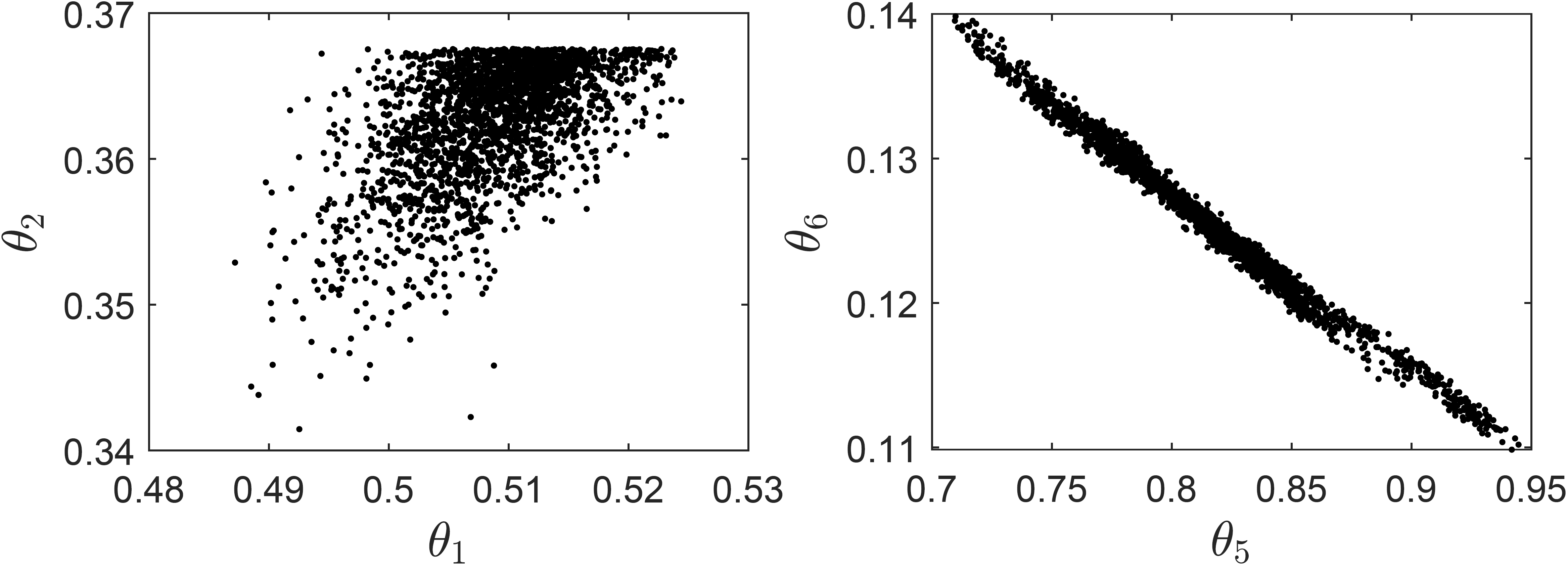
Refer to caption
Figure 10: Pairwise marginal samples from π\pi.

\begin{array}[]{cc}\vskip-5.69054pt\hskip-5.69054pt\includegraphics[width]{images/sec5_lossfunction-eps-converted-to.pdf}&\hskip-11.38109pt\includegraphics[width]{images/sec5_scaleadapt-eps-converted-to.pdf}\cr\end{array}

Figure 11: Convergence of GB MTM (solid lines) and LB MTM (dashed lines), with a log-scale on the xx-axis; all chains are started from the same state 𝜽0\boldsymbol{\theta}_{0} belonging to the tails of π\pi; left panel: trace plots of −log⁡π¯​(𝜽m|{𝐲k​(t)})-\log\bar{\pi}(\boldsymbol{\theta}_{m}\,|\,\{\mathbf{y}_{k}(t)\}) indicating the progress towards the high-probability region (designated by the dotted black line); right panel: adaptation of the step-size parameter ℓ\ell as the algorithms progress.

6 Discussion

In this paper, we revisited the promises and pitfalls of a popular MCMC method, namely MTM, through several new theoretical and empirical results. We proposed to use a novel class of weight functions, based on the so-called locally-balanced proposal distributions, that can be employed instead of the classical GB weight function without impacting neither the computational cost nor the coding complexity of MTM. The resulting LB MTM scheme is remarkably and positively different compared to the GB MTM one, especially regarding the behaviour of the induced Markov chains during the convergence phase. This difference is associated with substantially reduced burn-in time and an element of stability that, together with an easier tuning of the method, make LB MTM an appealing and competitive algorithm for high-dimensional Bayesian inference problems for which nothing except the unnormalized posterior density is known and when the latter is computationally expensive to evaluate, which makes in-step parallel computing beneficial.

Part of the research effort conducted in this paper can also be cast as an attempt to generalize the use of LB samplers beyond the discrete-state-space scenario. In particular, LB MTM is similar in spirit to exact-approximation schemes, in the sense of Andrieu and Vihola 2016, given that it can be thought of as approximations of ideal LB samplers that use a noisy version of the acceptance probability without affecting the invariant distribution. Further work in this direction is needed to explore these connections to strands of literature. Also, the results in this paper motivate further non-asymptotic (in NN and dd) theoretical analyses to identify other quantitative or qualitative differences between LB MTM algorithms and their GB counterpart. The rich literature on non-asymptotic analysis of MH exact-approximations (see, e.g., Andrieu and Vihola 2016, Andrieu et al. 2020, and Wang 2022) may prove useful in this direction.

While we have focused mainly on MTM and the impact of the weight function, it would be interesting to provide a systematic comparison of LB MTM with other multiple-proposal MCMC schemes (e.g., Neal 2003; Tjelmeland 2004; Frenkel 2004; Calderhead 2014; Holbrook 2023 and references therein) and more generally to other approaches that could in principle exploit in-step parallelization to speed-up convergence of MCMC. One such approach would be to exploit parallel target-density evaluations to derive numerical (e.g. finite-difference) approximations to the gradient, ∇log⁡π\nabla\log\pi, and then employ off-the-shelf gradient-based MCMC methods. We leave the exploration of such comparisons for future work, noting that it is likely that the optimal scheme among the ones mentioned above will depend on features of the target distribution (such as dimensionality, smoothness and regularity), and on the parallel-computing environment available (see, e.g., Glatt-Holtz et al. 2022 for examples of GPU implementations of multiple-proposal MCMC methods with large values of NN) as well as potentially other aspects.

Acknowledgments

Philippe Gagnon acknowledges support from NSERC (Natural Sciences and Engineering Research Council of Canada) and FRQNT (Fonds de recherche du Québec – Nature et technologies). Florian Maire acknowledges support from NSERC. Giacomo Zanella acknowledges support from the European Research Council (ERC), through StG “PrSc-HDBayLe” grant ID 101076564. Also, the authors thank three anonymous referees for helpful suggestions that led to an improved manuscript. The authors additionally thank Morgan Craig, professor in the Department of Mathematics and Statistics of Université de Montréal, for an introduction to the use of dynamical systems in precision medicine and for computer code to numerically solve the system of intermediate ordinary differential equations in the application of Section 5.

References

  • Andrieu and Thoms (2008) Andrieu, C. and Thoms, J. (2008) A tutorial on adaptive MCMC. Stat. Comput., 18, 343–373.
  • Andrieu and Vihola (2016) Andrieu, C. and Vihola, M. (2016) Establishing some order amongst exact approximations of MCMCs. Ann. Appl. Probab., 26, 2661–2696.
  • Andrieu et al. (2020) Andrieu, C., Yıldırım, S., Doucet, A. and Chopin, N. (2020) Metropolis–Hastings with averaged acceptance ratios. arXiv:2101.01253.
  • Barker (1965) Barker, A. A. (1965) Monte Carlo calculations of the radial distribution functions for a proton-electron plasma. Austral. J. Phys., 18, 119–134.
  • Bédard (2007) Bédard, M. (2007) Weak convergence of Metropolis algorithms for non-i.i.d. target distributions. Ann. Appl. Probab., 17, 1222–1244.
  • Bédard et al. (2012) Bédard, M., Douc, R. and Moulines, E. (2012) Scaling analysis of multiple-try MCMC methods. Stochastic Process. Appl., 122, 758–786.
  • Bou-Rabee and Hairer (2013) Bou-Rabee, N. and Hairer, M. (2013) Nonasymptotic mixing of the MALA algorithm. IMA J. Numer. Anal., 33, 80–110.
  • Bubeck (2015) Bubeck, S. (2015) Convex optimization: Algorithms and complexity. Foundations and Trends® in Machine Learning, 8, 231–357.
  • Calderhead (2014) Calderhead, B. (2014) A general construction for parallelizing Metropolis–Hastings algorithms. Proceedings of the National Academy of Sciences, 111, 17408–17413.
  • Chang et al. (2022) Chang, H., Lee, C. J., Luo, Z. T., Sang, H. and Zhou, Q. (2022) Rapidly mixing multiple-try Metropolis algorithms for model selection problems. Advances in Neural Information Processing Systems, 36.
  • Durmus et al. (2017) Durmus, A., Le Corff, S., Moulines, E. and Roberts, G. O. (2017) Optimal scaling of the random walk Metropolis algorithm under lpl^{p} mean differentiability. J. Appl. Probab., 54, 1233–1260.
  • Dwivedi et al. (2018) Dwivedi, R., Chen, Y., Wainwright, M. J. and Yu, B. (2018) Log-concave sampling: Metropolis–Hastings algorithms are fast! In Conference on learning theory, 793–797. PMLR.
  • Ethier and Kurtz (1986) Ethier, S. N. and Kurtz, T. G. (1986) Markov Processes: Characterization and Convergence. Wiley.
  • Frenkel (2004) Frenkel, D. (2004) Speed-up of Monte Carlo simulations by sampling of rejected states. Proceedings of the National Academy of Sciences, 101, 17571–17575.
  • Gagnon (2021) Gagnon, P. (2021) Informed reversible jump algorithms. Electron. J. Stat., 15, 3951–3995.
  • Gagnon et al. (2019) Gagnon, P., Bédard, M. and Desgagné, A. (2019) Weak convergence and optimal tuning of the reversible jump algorithm. Math. Comput. Simulation, 161, 32–51.
  • Gagnon and Maire (2020) Gagnon, P. and Maire, F. (2020) An asymptotic Peskun ordering and its application to lifted samplers. arXiv:2003.05492.
  • Glatt-Holtz et al. (2022) Glatt-Holtz, N. E., Holbrook, A. J., Krometis, J. A. and Mondaini, C. F. (2022) Parallel MCMC algorithms: Theoretical foundations, algorithm design, case studies. arXiv:2209.04750.
  • Hastings (1970) Hastings, W. K. (1970) Monte Carlo sampling methods using Markov chains and their applications. Biometrika, 57, 97–109.
  • Hird et al. (2022) Hird, M., Livingstone, S. and Zanella, G. (2022) A fresh take on ‘Barker dynamics’ for MCMC. In International Conference on Monte Carlo and Quasi-Monte Carlo Methods in Scientific Computing, 169–184. Springer.
  • Holbrook (2023) Holbrook, A. J. (2023) Generating MCMC proposals by randomly rotating the regular simplex. J. Multivariate Anal., 194, 1–15.
  • Huggins (2014) Huggins, J. H. (2014) An information-theoretic analysis of resampling in sequential Monte Carlo. Master’s thesis, Massachusetts Institute of Technology.
  • Jacob et al. (2020) Jacob, P. E., O’Leary, J. and Atchadé, Y. F. (2020) Unbiased Markov chain Monte Carlo methods with couplings. J. R. Stat. Soc. Ser. B. Stat. Methodol., 82, 543–600.
  • Jenner et al. (2021) Jenner, A. L., Cassidy, T., Belaid, K., Bourgeois-Daigneault, M.-C. and Craig, M. (2021) In silico trials predict that combination strategies for enhancing vesicular stomatitis oncolytic virus are determined by tumor aggressivity. Journal for immunotherapy of cancer, 9, 1–13.
  • Karr (1975) Karr, A. F. (1975) Weak convergence of a sequence of Markov chains. Z. Wahrsch. Verw. Gebiete, 33, 41–48.
  • Liang et al. (2022) Liang, X., Livingstone, S. and Griffin, J. (2022) Adaptive random neighbourhood informed Markov chain Monte Carlo for high-dimensional Bayesian variable selection. Stat. Comput., 32, 1–52.
  • Liu et al. (2000) Liu, J. S., Liang, F. and Wong, W. H. (2000) The multiple-try method and local optimization in Metropolis sampling. J. Amer. Statist. Assoc., 95, 121–134.
  • Livingstone and Zanella (2022) Livingstone, S. and Zanella, G. (2022) The Barker proposal: combining robustness and efficiency in gradient-based MCMC. J. R. Stat. Soc. Ser. B. Stat. Methodol., 84, 496–523.
  • Martino and Louzada (2017) Martino, L. and Louzada, F. (2017) Issues in the multiple try Metropolis mixing. Comput. Statist., 32, 239–252.
  • Metropolis et al. (1953) Metropolis, N., Rosenbluth, A. W., Rosenbluth, M. N., Teller, A. H. and Teller, E. (1953) Equation of state calculations by fast computing machines. J. Chem. Phys., 21, 1087–1092.
  • Müller and Stoyan (2002) Müller, A. and Stoyan, D. (2002) Comparison methods for stochastic models and risks. John Wiley & Sons Ltd., Chichester.
  • Neal (2003) Neal, R. M. (2003) Markov chain sampling for non-linear state space models using embedded hidden markov models. arXiv preprint math/0305039.
  • Pandolfi et al. (2010) Pandolfi, S., Bartolucci, F. and Friel, N. (2010) A generalization of the Multiple-try Metropolis algorithm for Bayesian estimation and model selection. In International Conference on Artificial Intelligence and Statistics, 581–588.
  • Power and Goldman (2019) Power, S. and Goldman, J. V. (2019) Accelerated sampling on discrete spaces with non-reversible markov processes. arXiv preprint arXiv:1912.04681.
  • Roberts et al. (1997) Roberts, G. O., Gelman, A. and Gilks, W. R. (1997) Weak convergence and optimal scaling of random walk Metropolis algorithms. Ann. Appl. Probab., 7, 110–120.
  • Roberts and Rosenthal (1998) Roberts, G. O. and Rosenthal, J. S. (1998) Optimal scaling of discrete approximations to Langevin diffusions. J. R. Stat. Soc. Ser. B. Stat. Methodol., 60, 255–268.
  • Roberts and Tweedie (1996) Roberts, G. O. and Tweedie, R. L. (1996) Exponential convergence of Langevin distributions and their discrete approximations. Bernoulli, 2, 341–363.
  • Rosenthal (2000) Rosenthal, J. S. (2000) Parallel computing and Monte Carlo algorithms. Far East J. Theor. Stat., 4, 207–236.
  • Sansone (2022) Sansone, E. (2022) LSB: Local self-balancing MCMC in discrete spaces. In International Conference on Machine Learning, 19205–19220. PMLR.
  • Schmon et al. (2021) Schmon, S. M., Deligiannidis, G., Doucet, A. and Pitt, M. K. (2021) Large-sample asymptotics of the pseudo-marginal method. Biometrika, 108, 37–51.
  • Schmon and Gagnon (2022) Schmon, S. M. and Gagnon, P. (2022) Optimal scaling of random walk Metropolis algorithms using Bayesian large-sample asymptotics. Stat. Comput., 32, 1–16.
  • Sun et al. (2022a) Sun, H., Dai, H., Dai, B., Zhou, H. and Schuurmans, D. (2022a) Discrete Langevin sampler via Wasserstein gradient flow. arXiv:2206.14897.
  • Sun et al. (2022b) Sun, H., Dai, H. and Schuurmans, D. (2022b) Optimal scaling for locally balanced proposals in discrete spaces. arXiv:2209.08183.
  • Sun et al. (2021) Sun, H., Dai, H., Xia, W. and Ramamurthy, A. (2021) Path auxiliary proposal for MCMC in discrete space. In International Conference on Learning Representations.
  • Tjelmeland (2004) Tjelmeland, H. (2004) Using all Metropolis–Hastings proposals to estimate mean values. Tech. rep.
  • Vogrinc et al. (2023) Vogrinc, J., Livingstone, S. and Zanella, G. (2023) Optimal design of the Barker proposal and other locally-balanced Metropolis–Hastings algorithms. To appear in Biometrika.
  • Wang (2022) Wang, G. (2022) On the theoretical properties of the Exchange algorithm. Bernoulli, 28, 1935–1960.
  • Zanella (2020) Zanella, G. (2020) Informed proposals for local MCMC in discrete spaces. J. Amer. Statist. Assoc., 115, 852–865.
  • Zhou and Smith (2022) Zhou, Q. and Smith, A. (2022) Rapid convergence of informed importance tempering. In International Conference on Artificial Intelligence and Statistics, 10939–10965. PMLR.

Appendix A Proofs

Proof of Proposition 1.

First, let us look at

ℙ𝐱(J=j∣𝐘1,…,𝐘N)=𝔼𝐱[𝟙J=j∣𝐘1,…,𝐘N]=w⁡(𝐱,𝐘j)∑i=1Nw⁡(𝐱,𝐘i).\mathbb{P}_{\mathbf{x}}(J=j\mid\mathbf{Y}_{1},\ldots,\mathbf{Y}_{N})=\mathbb{E}_{\mathbf{x}}[\mathbbm{1}_{J=j}\mid\mathbf{Y}_{1},\ldots,\mathbf{Y}_{N}]=\frac{w(\mathbf{x},\mathbf{Y}_{j})}{\sum_{i=1}^{N}w(\mathbf{x},\mathbf{Y}_{i})}.

Using this and that 𝐘1,…,𝐘N\mathbf{Y}_{1},\ldots,\mathbf{Y}_{N} are conditionally IID given 𝐱\mathbf{x}, we have that

𝔼𝐱​[h⁡(𝐘J)]=∑j=1N𝔼𝐱​[h⁡(𝐘j)​ 1J=j]\displaystyle\mathbb{E}_{\mathbf{x}}[h(\mathbf{Y}_{J})]=\sum_{j=1}^{N}\mathbb{E}_{\mathbf{x}}[h(\mathbf{Y}_{j})\,\mathbbm{1}_{J=j}] =∑j=1N𝔼𝐱[h(𝐘j)𝔼[𝟙J=j∣𝐘1,…,𝐘N]]\displaystyle=\sum_{j=1}^{N}\mathbb{E}_{\mathbf{x}}[h(\mathbf{Y}_{j})\,\mathbb{E}[\mathbbm{1}_{J=j}\mid\mathbf{Y}_{1},\ldots,\mathbf{Y}_{N}]]
=∑j=1N𝔼𝐱​[h⁡(𝐘j)​w⁡(𝐱,𝐘j)∑i=1Nw⁡(𝐱,𝐘i)]\displaystyle=\sum_{j=1}^{N}\mathbb{E}_{\mathbf{x}}\left[h(\mathbf{Y}_{j})\,\frac{w(\mathbf{x},\mathbf{Y}_{j})}{\sum_{i=1}^{N}w(\mathbf{x},\mathbf{Y}_{i})}\right]
=∑j=1N∫h(𝐲j)w⁡(𝐱,𝐲j)∑i=1Nw⁡(𝐱,𝐲i)∏i=1Nqσd(𝐱,𝐲i)d𝐲1:N\displaystyle=\sum_{j=1}^{N}\int h(\mathbf{y}_{j})\,\frac{w(\mathbf{x},\mathbf{y}_{j})}{\sum_{i=1}^{N}w(\mathbf{x},\mathbf{y}_{i})}\prod_{i=1}^{N}q_{\sigma_{d}}(\mathbf{x},\mathbf{y}_{i})\,\mathrm{d}\mathbf{y}_{1:N}
=∫h(𝐲1)w⁡(𝐱,𝐲1)1N​∑i=1Nw⁡(𝐱,𝐲i)∏i=1Nqσd(𝐱,𝐲i)d𝐲1:N.\displaystyle=\int h(\mathbf{y}_{1})\,\frac{w(\mathbf{x},\mathbf{y}_{1})}{\frac{1}{N}\sum_{i=1}^{N}w(\mathbf{x},\mathbf{y}_{i})}\prod_{i=1}^{N}q_{\sigma_{d}}(\mathbf{x},\mathbf{y}_{i})\,\mathrm{d}\mathbf{y}_{1:N}.

∎

A.1 Proof of Theorem 1

In order to prove Theorem 1, we provide a general convergence result.

Theorem 4.

Let {PN:N≥1}\{P_{N}:N\geq 1\} be a collection of Markov transition kernels and PP a Markov transition kernel such that PNP_{N} (for any NN) and PP admit π\pi as invariant distribution. If the following assumptions hold:

(a)

the Markov transition kernels {PN:N≥1}\{P_{N}:N\geq 1\} satisfy

∫|PN​h​(𝐱)−P​h​(𝐱)|​π​(𝐱)​𝑑𝐱→0\int|P_{N}h(\mathbf{x})-Ph(\mathbf{x})|\,\pi(\mathbf{x})\,\mathrm{d}\mathbf{x}\rightarrow 0

as N→∞N\rightarrow\infty for all h∈𝒞bh\in\mathcal{C}_{\text{b}}, where

PN​h​(𝐱):=∫PN​(𝐱,𝑑𝐲)​h​(𝐲),P_{N}h(\mathbf{x}):=\int P_{N}(\mathbf{x},\mathrm{d}\mathbf{y})\,h(\mathbf{y}),

with an analogous definition for P​hPh, 𝒞b\mathcal{C}_{\text{b}} being the space of bounded continuous functions;

(b)

P​hPh is continuous for any h∈𝒞bh\in\mathcal{C}_{\text{b}},

then {𝐗N​(m):m∈ℕ}\{\mathbf{X}_{N}(m):m\in\N\} converges weakly to {𝐗⁡(m):m∈ℕ}\{\mathbf{X}(m):m\in\N\} provided that 𝐗N​(0)∼π\mathbf{X}_{N}(0)\sim\pi and 𝐗⁡(0)∼π\mathbf{X}(0)\sim\pi, {𝐗N​(m):m∈ℕ}\{\mathbf{X}_{N}(m):m\in\N\} and {𝐗⁡(m):m∈ℕ}\{\mathbf{X}(m):m\in\N\} being the Markov chains with transition kernels PNP_{N} and PP, respectively.

We present a proof here for self-containedness, but do not claim the originality of the result. The proof is strongly inspired by that of Theorem 2 in Schmon et al. 2021.

Proof.

To prove that {𝐗N​(m):m∈ℕ}\{\mathbf{X}_{N}(m):m\in\N\} converges weakly to {𝐗⁡(m):m∈ℕ}\{\mathbf{X}(m):m\in\N\}, we only need to prove the convergence of finite-dimensional distributions (Karr 1975). It thus suffices to prove that for any positive integer kk

|𝔼⁡[f0​(𝐗N​(0))​…​fk​(𝐗N​(k))]−𝔼⁡[f0​(𝐗⁡(0))​…​fk​(𝐗⁡(k))]|→0,|\mathbb{E}[f_{0}(\mathbf{X}_{N}(0))\ldots f_{k}(\mathbf{X}_{N}(k))]-\mathbb{E}[f_{0}(\mathbf{X}(0))\ldots f_{k}(\mathbf{X}(k))]|\rightarrow 0,

as N→∞N\rightarrow\infty, for all f0,…,fk∈𝒞bf_{0},\ldots,f_{k}\in\mathcal{C}_{\text{b}} given that (𝐱⁡(0),…,𝐱⁡(k))↦∏i=0kfi​(𝐱⁡(i))(\mathbf{x}(0),\ldots,\mathbf{x}(k))\mapsto\prod_{i=0}^{k}f_{i}(\mathbf{x}(i)) is measure determining by Proposition 4.6 in Chapter 2 of Ethier and Kurtz 1986.

We prove this by induction. For k=0k=0, the convergence is trivial because 𝐗N​(0)∼π\mathbf{X}_{N}(0)\sim\pi and 𝐗⁡(0)∼π\mathbf{X}(0)\sim\pi. Now assume that it is true for k≥0k\geq 0, and let us verify that it is true for k+1k+1.

|𝔼⁡[f0​(𝐗N​(0))​…​fk​(𝐗N​(k))​fk+1​(𝐗N​(k+1))]−𝔼⁡[f0​(𝐗⁡(0))​…​fk​(𝐗⁡(k))​fk+1​(𝐗⁡(k+1))]|\displaystyle|\mathbb{E}[f_{0}(\mathbf{X}_{N}(0))\ldots f_{k}(\mathbf{X}_{N}(k))f_{k+1}(\mathbf{X}_{N}(k+1))]-\mathbb{E}[f_{0}(\mathbf{X}(0))\ldots f_{k}(\mathbf{X}(k))f_{k+1}(\mathbf{X}(k+1))]|
=|𝔼⁡[f0​(𝐗N​(0))​…​fk​(𝐗N​(k))​PN​fk+1​(𝐗N​(k))]−𝔼⁡[f0​(𝐗⁡(0))​…​fk​(𝐗⁡(k))​P​fk+1​(𝐗⁡(k))]|\displaystyle=|\mathbb{E}[f_{0}(\mathbf{X}_{N}(0))\ldots f_{k}(\mathbf{X}_{N}(k))P_{N}f_{k+1}(\mathbf{X}_{N}(k))]-\mathbb{E}[f_{0}(\mathbf{X}(0))\ldots f_{k}(\mathbf{X}(k))Pf_{k+1}(\mathbf{X}(k))]|
≤|𝔼⁡[f0​(𝐗N​(0))​…​fk​(𝐗N​(k))​PN​fk+1​(𝐗N​(k))−f0​(𝐗N​(0))​…​fk​(𝐗N​(k))​P​fk+1​(𝐗N​(k))]|\displaystyle\leq|\mathbb{E}[f_{0}(\mathbf{X}_{N}(0))\ldots f_{k}(\mathbf{X}_{N}(k))P_{N}f_{k+1}(\mathbf{X}_{N}(k))-f_{0}(\mathbf{X}_{N}(0))\ldots f_{k}(\mathbf{X}_{N}(k))Pf_{k+1}(\mathbf{X}_{N}(k))]|
+|𝔼⁡[f0​(𝐗N​(0))​…​fk​(𝐗N​(k))​P​fk+1​(𝐗N​(k))]−𝔼⁡[f0​(𝐗⁡(0))​…​fk​(𝐗⁡(k))​P​fk+1​(𝐗⁡(k))]|\displaystyle\quad+|\mathbb{E}[f_{0}(\mathbf{X}_{N}(0))\ldots f_{k}(\mathbf{X}_{N}(k))Pf_{k+1}(\mathbf{X}_{N}(k))]-\mathbb{E}[f_{0}(\mathbf{X}(0))\ldots f_{k}(\mathbf{X}(k))Pf_{k+1}(\mathbf{X}(k))]|
≤Mk​𝔼​[|PN​fk+1​(𝐗N​(k))−P​fk+1​(𝐗N​(k))|]\displaystyle\leq M^{k}\mathbb{E}[|P_{N}f_{k+1}(\mathbf{X}_{N}(k))-Pf_{k+1}(\mathbf{X}_{N}(k))|]
+|𝔼⁡[f0​(𝐗N​(0))​…​fk​(𝐗N​(k))​P​fk+1​(𝐗N​(k))]−𝔼⁡[f0​(𝐗⁡(0))​…​fk​(𝐗⁡(k))​P​fk+1​(𝐗⁡(k))]|,\displaystyle\quad+|\mathbb{E}[f_{0}(\mathbf{X}_{N}(0))\ldots f_{k}(\mathbf{X}_{N}(k))Pf_{k+1}(\mathbf{X}_{N}(k))]-\mathbb{E}[f_{0}(\mathbf{X}(0))\ldots f_{k}(\mathbf{X}(k))Pf_{k+1}(\mathbf{X}(k))]|,

using that there exists a positive constant MM such that fi≤Mf_{i}\leq M for all ii. The term on the penultimate line vanishes as a consequence of Assumption (a). That on the last line vanishes because P​fk+1Pf_{k+1} is bounded and continuous by Assumption (b). ∎

Before presenting the proof of Theorem 1, we present a result that will be used in it and in other proofs.

Proposition 4.

(Müller and Stoyan 2002, Corollary 1.5.24) For any N≥2N\geq 2 exchangeable random variables X1,…,XNX_{1},\ldots,X_{N} and any convex function ϕ\phi, we have

𝔼⁡[ϕ⁡(1N​∑i=1NXi)]≤𝔼⁡[ϕ⁡(1N−1​∑i=1N−1Xi)],\mathbb{E}\left[\phi\left(\frac{1}{N}\sum_{i=1}^{N}X_{i}\right)\right]\leq\mathbb{E}\left[\phi\left(\frac{1}{N-1}\sum_{i=1}^{N-1}X_{i}\right)\right],

whenever the expectations exist.

Proof of Theorem 1.

We start with Result 1. The strategy to prove the result is the same as that to prove Theorem 2.1.1 in Huggins 2014. The probability that 𝐘J\mathbf{Y}_{J} belongs to a set AA, for fixed 𝐱\mathbf{x}, as a function of NN is

Qw,σN​(𝐱,A):=ℙ𝐱,N​(𝐘J∈A)=𝔼𝐱​[𝟙𝐘1∈A​w⁡(𝐱,𝐘1)1N​∑i=1Nw⁡(𝐱,𝐘i)],Q_{w,\sigma}^{N}(\mathbf{x},A):=\mathbb{P}_{\mathbf{x},N}(\mathbf{Y}_{J}\in A)=\mathbb{E}_{\mathbf{x}}\left[\mathbbm{1}_{\mathbf{Y}_{1}\in A}\,\frac{w(\mathbf{x},\mathbf{Y}_{1})}{\frac{1}{N}\sum_{i=1}^{N}w(\mathbf{x},\mathbf{Y}_{i})}\right],

using Proposition 1. To simplify the notation for this part of the proof, we omit the dependence on w,σw,\sigma and 𝐱\mathbf{x} that are fixed throughout, and use QN​(A):=Qw,σN​(𝐱,A)Q^{N}(A):=Q_{w,\sigma}^{N}(\mathbf{x},A) and Q⁡(A):=Qw,σ​(𝐱,A)Q(A):=Q_{w,\sigma}(\mathbf{x},A).

We have that

QN​(A)\displaystyle Q^{N}(A) =𝔼𝐱​[𝟙𝐘1∈A​w​(𝐱,𝐘1)​𝔼𝐱​[11N​∑i=1Nw⁡(𝐱,𝐘i)∣𝐘1]].\displaystyle=\mathbb{E}_{\mathbf{x}}\left[\mathbbm{1}_{\mathbf{Y}_{1}\in A}\,w(\mathbf{x},\mathbf{Y}_{1})\,\mathbb{E}_{\mathbf{x}}\left[\frac{1}{\frac{1}{N}\sum_{i=1}^{N}w(\mathbf{x},\mathbf{Y}_{i})}\mid\mathbf{Y}_{1}\right]\right].

With

h⁡(𝐘1):=𝔼𝐱​[11N​∑i=1Nw⁡(𝐱,𝐘i)∣𝐘1],h(\mathbf{Y}_{1}):=\mathbb{E}_{\mathbf{x}}\left[\frac{1}{\frac{1}{N}\sum_{i=1}^{N}w(\mathbf{x},\mathbf{Y}_{i})}\mid\mathbf{Y}_{1}\right],

we have that

QN​(A)=𝔼𝐱​[𝟙𝐘1∈A​w​(𝐱,𝐘1)​h​(𝐘1)]\displaystyle Q^{N}(A)=\mathbb{E}_{\mathbf{x}}\left[\mathbbm{1}_{\mathbf{Y}_{1}\in A}\,w(\mathbf{x},\mathbf{Y}_{1})\,h(\mathbf{Y}_{1})\right] =∫Aw⁡(𝐱,𝐲1)​h​(𝐲1)​qσ​(𝐱,𝐲1)​d​𝐲1\displaystyle=\int_{A}w(\mathbf{x},\mathbf{y}_{1})\,h(\mathbf{y}_{1})\,q_{\sigma}(\mathbf{x},\mathbf{y}_{1})\,\mathrm{d}\mathbf{y}_{1}
=∫A𝔼𝐱​[w⁡(𝐱,𝐘1)]​h​(𝐲1)​Qw,σ​(𝐱,𝐲1)​d​𝐲1.\displaystyle=\int_{A}\mathbb{E}_{\mathbf{x}}[w(\mathbf{x},\mathbf{Y}_{1})]\,h(\mathbf{y}_{1})\,Q_{w,\sigma}(\mathbf{x},\mathbf{y}_{1})\,\mathrm{d}\mathbf{y}_{1}.

This implies that we have an expression for the following Radon–Nikodym derivative:

d​QNd​Q​(𝐲1)\displaystyle\frac{\mathrm{d}Q^{N}}{\mathrm{d}Q}(\mathbf{y}_{1}) =𝔼𝐱​[w⁡(𝐱,𝐘1)]​𝔼𝐱​[11N​∑i=1Nw⁡(𝐱,𝐘i)∣𝐘1=𝐲1]\displaystyle=\mathbb{E}_{\mathbf{x}}[w(\mathbf{x},\mathbf{Y}_{1})]\mathbb{E}_{\mathbf{x}}\left[\frac{1}{\frac{1}{N}\sum_{i=1}^{N}w(\mathbf{x},\mathbf{Y}_{i})}\mid\mathbf{Y}_{1}=\mathbf{y}_{1}\right]
≥𝔼𝐱​[w⁡(𝐱,𝐘1)]1N​∑i=1N𝔼𝐱​[w⁡(𝐱,𝐘i)∣𝐘1=𝐲1]\displaystyle\geq\frac{\mathbb{E}_{\mathbf{x}}[w(\mathbf{x},\mathbf{Y}_{1})]}{\frac{1}{N}\sum_{i=1}^{N}\mathbb{E}_{\mathbf{x}}[w(\mathbf{x},\mathbf{Y}_{i})\mid\mathbf{Y}_{1}=\mathbf{y}_{1}]}
=N​𝔼𝐱​[w⁡(𝐱,𝐘1)](N−1)​𝔼𝐱​[w⁡(𝐱,𝐘1)]+w⁡(𝐱,𝐲1),\displaystyle=\frac{N\mathbb{E}_{\mathbf{x}}[w(\mathbf{x},\mathbf{Y}_{1})]}{(N-1)\mathbb{E}_{\mathbf{x}}[w(\mathbf{x},\mathbf{Y}_{1})]+w(\mathbf{x},\mathbf{y}_{1})},

using Jensen’s inequality.

To prove Result 1, we use that the total variation between QN​(A)Q^{N}(A) and Q⁡(A)Q(A) can be bounded above using the Kullback–Leibler divergence, and more precisely, by

12​∫Q⁡(𝐲1)​d​𝐲1​log⁡d​Qd​QN​(𝐲1).\sqrt{\frac{1}{2}\int Q(\mathbf{y}_{1})\,\mathrm{d}\mathbf{y}_{1}\log\frac{\mathrm{d}Q}{\mathrm{d}Q^{N}}(\mathbf{y}_{1})}.

We have that

∫Q⁡(𝐲1)​d​𝐲1​log⁡d​Q​(𝐲1)d​QN​(𝐲1)\displaystyle\int Q(\mathbf{y}_{1})\,\mathrm{d}\mathbf{y}_{1}\log\frac{\mathrm{d}Q(\mathbf{y}_{1})}{\mathrm{d}Q^{N}(\mathbf{y}_{1})} ≤∫Q⁡(𝐲1)​d​𝐲1​log⁡(N−1)​𝔼𝐱​[w⁡(𝐱,𝐘1)]+w⁡(𝐱,𝐲1)N​𝔼𝐱​[w⁡(𝐱,𝐘1)]\displaystyle\leq\int Q(\mathbf{y}_{1})\,\mathrm{d}\mathbf{y}_{1}\log\frac{(N-1)\mathbb{E}_{\mathbf{x}}[w(\mathbf{x},\mathbf{Y}_{1})]+w(\mathbf{x},\mathbf{y}_{1})}{N\mathbb{E}_{\mathbf{x}}[w(\mathbf{x},\mathbf{Y}_{1})]}
≤log∫Q(𝐲1)d𝐲1(N−1)​𝔼𝐱​[w⁡(𝐱,𝐘1)]+w⁡(𝐱,𝐲1)N​𝔼𝐱​[w⁡(𝐱,𝐘1)]\displaystyle\leq\log\int Q(\mathbf{y}_{1})\,\mathrm{d}\mathbf{y}_{1}\frac{(N-1)\mathbb{E}_{\mathbf{x}}[w(\mathbf{x},\mathbf{Y}_{1})]+w(\mathbf{x},\mathbf{y}_{1})}{N\mathbb{E}_{\mathbf{x}}[w(\mathbf{x},\mathbf{Y}_{1})]}
=log⁡(1+∫w⁡(𝐱,𝐲1)​Q​(𝐲1)​d​𝐲1−𝔼𝐱​[w⁡(𝐱,𝐘1)]N​𝔼𝐱​[w⁡(𝐱,𝐘1)])\displaystyle=\log\left(1+\frac{\int w(\mathbf{x},\mathbf{y}_{1})Q(\mathbf{y}_{1})\,\mathrm{d}\mathbf{y}_{1}-\mathbb{E}_{\mathbf{x}}[w(\mathbf{x},\mathbf{Y}_{1})]}{N\mathbb{E}_{\mathbf{x}}[w(\mathbf{x},\mathbf{Y}_{1})]}\right)
=log⁡(1+∫w​(𝐱,𝐲1)2​qσ​(𝐱,𝐲1)​d​𝐲1−𝔼𝐱​[w⁡(𝐱,𝐘1)]2N​𝔼𝐱​[w⁡(𝐱,𝐘1)]2)\displaystyle=\log\left(1+\frac{\int w(\mathbf{x},\mathbf{y}_{1})^{2}q_{\sigma}(\mathbf{x},\mathbf{y}_{1})\,\mathrm{d}\mathbf{y}_{1}-\mathbb{E}_{\mathbf{x}}[w(\mathbf{x},\mathbf{Y}_{1})]^{2}}{N\mathbb{E}_{\mathbf{x}}[w(\mathbf{x},\mathbf{Y}_{1})]^{2}}\right)
≤var𝐱​[w⁡(𝐱,𝐘1)]N​𝔼𝐱​[w⁡(𝐱,𝐘1)]2,\displaystyle\leq\frac{\hbox{var}_{\mathbf{x}}[w(\mathbf{x},\mathbf{Y}_{1})]}{N\mathbb{E}_{\mathbf{x}}[w(\mathbf{x},\mathbf{Y}_{1})]^{2}},

using Jensen’s inequality and that log⁡(1+x)≤x\log(1+x)\leq x for all x>−1x>-1. This concludes the proof of Result 1 as, by assumption 𝔼𝐱​[w​(𝐱,𝐘1)4]<∞\mathbb{E}_{\mathbf{x}}\left[w(\mathbf{x},\mathbf{Y}_{1})^{4}\right]<\infty, and 𝔼𝐱​[w⁡(𝐱,𝐘1)]>0\mathbb{E}_{\mathbf{x}}[w(\mathbf{x},\mathbf{Y}_{1})]>0 given that ww is a strictly positive function.

We now prove Result 2. To achieve this, we use Theorem 4, which requires that:

(a)

for every h∈𝒞bh\in\mathcal{C}_{\text{b}} (the space of bounded continuous functions),

∫|PN​h​(𝐱)−Pideal​h​(𝐱)|​π​(𝐱)​𝑑𝐱→0,\int|P_{N}h(\mathbf{x})-P_{\text{ideal}}h(\mathbf{x})|\,\pi(\mathbf{x})\,\mathrm{d}\mathbf{x}\rightarrow 0,

where PNP_{N} is the Markov kernel simulated by MTM and PidealP_{\text{ideal}} is the Markov kernel simulated by the ideal scheme;

(b)

Pideal​hP_{\text{ideal}}h is continuous for any h∈𝒞bh\in\mathcal{C}_{\text{b}}.

Let us first define PNP_{N} and PidealP_{\text{ideal}}:

PN(𝐱,A):=∑j=1N∫𝐲j∈Aw⁡(𝐱,𝐲j)∑i=1Nw⁡(𝐱,𝐲i)∏i=1Nqσ(𝐱,𝐲i)∏i=1N−1qσ(𝐲j,𝐳i)α(𝐱,𝐲j)d(𝐲1:N,𝐳1:N−1)\displaystyle P_{N}(\mathbf{x},A):=\sum_{j=1}^{N}\int_{\mathbf{y}_{j}\in A}\frac{w(\mathbf{x},\mathbf{y}_{j})}{\sum_{i=1}^{N}w(\mathbf{x},\mathbf{y}_{i})}\prod_{i=1}^{N}q_{\sigma}(\mathbf{x},\mathbf{y}_{i})\prod_{i=1}^{N-1}q_{\sigma}(\mathbf{y}_{j},\mathbf{z}_{i})\,\alpha(\mathbf{x},\mathbf{y}_{j})\,\mathrm{d}(\mathbf{y}_{1:N},\mathbf{z}_{1:N-1})
+𝟙𝐱∈A∑j=1N∫w⁡(𝐱,𝐲j)∑i=1Nw⁡(𝐱,𝐲i)∏i=1Nqσ(𝐱,𝐲i)∏i=1N−1qσ(𝐲j,𝐳i)(1−α(𝐱,𝐲j))d(𝐲1:N,𝐳1:N−1),\displaystyle\qquad+\mathbbm{1}_{\mathbf{x}\in A}\sum_{j=1}^{N}\int\frac{w(\mathbf{x},\mathbf{y}_{j})}{\sum_{i=1}^{N}w(\mathbf{x},\mathbf{y}_{i})}\prod_{i=1}^{N}q_{\sigma}(\mathbf{x},\mathbf{y}_{i})\prod_{i=1}^{N-1}q_{\sigma}(\mathbf{y}_{j},\mathbf{z}_{i})\,(1-\alpha(\mathbf{x},\mathbf{y}_{j}))\,\mathrm{d}(\mathbf{y}_{1:N},\mathbf{z}_{1:N-1}),

and

Pideal​(𝐱,A):=∫𝐲∈AQw,σ​(𝐱,𝐲)​αideal​(𝐱,𝐲)​𝑑𝐲+𝟙𝐱∈A​∫Qw,σ​(𝐱,𝐲)​(1−αideal​(𝐱,𝐲))​𝑑𝐲,\displaystyle P_{\text{ideal}}(\mathbf{x},A):=\int_{\mathbf{y}\in A}Q_{w,\sigma}(\mathbf{x},\mathbf{y})\,\alpha_{\text{ideal}}(\mathbf{x},\mathbf{y})\,\mathrm{d}\mathbf{y}+\mathbbm{1}_{\mathbf{x}\in A}\int Q_{w,\sigma}(\mathbf{x},\mathbf{y})\,(1-\alpha_{\text{ideal}}(\mathbf{x},\mathbf{y}))\,\mathrm{d}\mathbf{y},

where

αideal​(𝐱,𝐲):=1∧π⁡(𝐲)​Qw,σ​(𝐲,𝐱)π⁡(𝐱)​Qw,σ​(𝐱,𝐲).\alpha_{\text{ideal}}(\mathbf{x},\mathbf{y}):=1\wedge\frac{\pi(\mathbf{y})\,Q_{w,\sigma}(\mathbf{y},\mathbf{x})}{\pi(\mathbf{x})\,Q_{w,\sigma}(\mathbf{x},\mathbf{y})}.

In PN​(𝐱,A)P_{N}(\mathbf{x},A), the integrals are the same for all jj. Therefore,

PN(𝐱,A):=∫𝐲1∈Aw⁡(𝐱,𝐲1)1N​∑i=1Nw⁡(𝐱,𝐲i)∏i=1Nqσ(𝐱,𝐲i)∏i=1N−1qσ(𝐲1,𝐳i)α(𝐱,𝐲1)d(𝐲1:N,𝐳1:N−1)\displaystyle P_{N}(\mathbf{x},A):=\int_{\mathbf{y}_{1}\in A}\frac{w(\mathbf{x},\mathbf{y}_{1})}{\frac{1}{N}\sum_{i=1}^{N}w(\mathbf{x},\mathbf{y}_{i})}\prod_{i=1}^{N}q_{\sigma}(\mathbf{x},\mathbf{y}_{i})\prod_{i=1}^{N-1}q_{\sigma}(\mathbf{y}_{1},\mathbf{z}_{i})\,\alpha(\mathbf{x},\mathbf{y}_{1})\,\mathrm{d}(\mathbf{y}_{1:N},\mathbf{z}_{1:N-1})
+𝟙𝐱∈A∫w⁡(𝐱,𝐲1)1N​∑i=1Nw⁡(𝐱,𝐲i)∏i=1Nqσ(𝐱,𝐲i)∏i=1N−1qσ(𝐲1,𝐳i)(1−α(𝐱,𝐲1))d(𝐲1:N,𝐳1:N−1).\displaystyle\qquad+\mathbbm{1}_{\mathbf{x}\in A}\int\frac{w(\mathbf{x},\mathbf{y}_{1})}{\frac{1}{N}\sum_{i=1}^{N}w(\mathbf{x},\mathbf{y}_{i})}\prod_{i=1}^{N}q_{\sigma}(\mathbf{x},\mathbf{y}_{i})\prod_{i=1}^{N-1}q_{\sigma}(\mathbf{y}_{1},\mathbf{z}_{i})\,(1-\alpha(\mathbf{x},\mathbf{y}_{1}))\,\mathrm{d}(\mathbf{y}_{1:N},\mathbf{z}_{1:N-1}).

Consequently,

PNh(𝐱)=∫w⁡(𝐱,𝐲1)1N​∑i=1Nw⁡(𝐱,𝐲i)∏i=1Nqσ(𝐱,𝐲i)∏i=1N−1qσ(𝐲1,𝐳i)α(𝐱,𝐲1)h(𝐲1)d(𝐲1:N,𝐳1:N−1)\displaystyle P_{N}h(\mathbf{x})=\int\frac{w(\mathbf{x},\mathbf{y}_{1})}{\frac{1}{N}\sum_{i=1}^{N}w(\mathbf{x},\mathbf{y}_{i})}\prod_{i=1}^{N}q_{\sigma}(\mathbf{x},\mathbf{y}_{i})\prod_{i=1}^{N-1}q_{\sigma}(\mathbf{y}_{1},\mathbf{z}_{i})\,\alpha(\mathbf{x},\mathbf{y}_{1})\,h(\mathbf{y}_{1})\,\mathrm{d}(\mathbf{y}_{1:N},\mathbf{z}_{1:N-1})
+h(𝐱)∫w⁡(𝐱,𝐲1)1N​∑i=1Nw⁡(𝐱,𝐲i)∏i=1Nqσ(𝐱,𝐲i)∏i=1N−1qσ(𝐲1,𝐳i)(1−α(𝐱,𝐲1))d(𝐲1:N,𝐳1:N−1),\displaystyle\qquad+h(\mathbf{x})\int\frac{w(\mathbf{x},\mathbf{y}_{1})}{\frac{1}{N}\sum_{i=1}^{N}w(\mathbf{x},\mathbf{y}_{i})}\prod_{i=1}^{N}q_{\sigma}(\mathbf{x},\mathbf{y}_{i})\prod_{i=1}^{N-1}q_{\sigma}(\mathbf{y}_{1},\mathbf{z}_{i})\,(1-\alpha(\mathbf{x},\mathbf{y}_{1}))\,\mathrm{d}(\mathbf{y}_{1:N},\mathbf{z}_{1:N-1}),

and

Pideal​h​(𝐱):=∫Qw,σ​(𝐱,𝐲)​αideal​(𝐱,𝐲)​h​(𝐲)​𝑑𝐲+h⁡(𝐱)​∫Qw,σ​(𝐱,𝐲)​(1−αideal​(𝐱,𝐲))​𝑑𝐲.\displaystyle P_{\text{ideal}}h(\mathbf{x}):=\int Q_{w,\sigma}(\mathbf{x},\mathbf{y})\,\alpha_{\text{ideal}}(\mathbf{x},\mathbf{y})\,h(\mathbf{y})\,\mathrm{d}\mathbf{y}+h(\mathbf{x})\int Q_{w,\sigma}(\mathbf{x},\mathbf{y})\,(1-\alpha_{\text{ideal}}(\mathbf{x},\mathbf{y}))\,\mathrm{d}\mathbf{y}. (10)

We first prove that

∫|PN​h​(𝐱)−Pideal​h​(𝐱)|​π​(𝐱)​𝑑𝐱→0.\int|P_{N}h(\mathbf{x})-P_{\text{ideal}}h(\mathbf{x})|\,\pi(\mathbf{x})\,\mathrm{d}\mathbf{x}\rightarrow 0.

Using the triangle inequality, it suffices to prove that

∫|∫w⁡(𝐱,𝐲1)1N​∑i=1Nw⁡(𝐱,𝐲i)∏i=1Nqσ(𝐱,𝐲i)∏i=1N−1qσ(𝐲1,𝐳i)α(𝐱,𝐲1)h(𝐲1)d(𝐲1:N,𝐳1:N−1)\displaystyle\int\left|\int\frac{w(\mathbf{x},\mathbf{y}_{1})}{\frac{1}{N}\sum_{i=1}^{N}w(\mathbf{x},\mathbf{y}_{i})}\prod_{i=1}^{N}q_{\sigma}(\mathbf{x},\mathbf{y}_{i})\prod_{i=1}^{N-1}q_{\sigma}(\mathbf{y}_{1},\mathbf{z}_{i})\,\alpha(\mathbf{x},\mathbf{y}_{1})\,h(\mathbf{y}_{1})\,\mathrm{d}(\mathbf{y}_{1:N},\mathbf{z}_{1:N-1})\right.
−∫Qw,σ(𝐱,𝐲)αideal(𝐱,𝐲)h(𝐲)d𝐲|π(𝐱)d𝐱→0,\displaystyle\qquad\left.-\int Q_{w,\sigma}(\mathbf{x},\mathbf{y})\,\alpha_{\text{ideal}}(\mathbf{x},\mathbf{y})\,h(\mathbf{y})\,\mathrm{d}\mathbf{y}\right|\,\pi(\mathbf{x})\,\mathrm{d}\mathbf{x}\rightarrow 0,

and

∫|h(𝐱)∫w⁡(𝐱,𝐲1)1N​∑i=1Nw⁡(𝐱,𝐲i)∏i=1Nqσ(𝐱,𝐲i)∏i=1N−1qσ(𝐲1,𝐳i)(1−α(𝐱,𝐲1))d(𝐲1:N,𝐳1:N−1)\displaystyle\int\left|h(\mathbf{x})\int\frac{w(\mathbf{x},\mathbf{y}_{1})}{\frac{1}{N}\sum_{i=1}^{N}w(\mathbf{x},\mathbf{y}_{i})}\prod_{i=1}^{N}q_{\sigma}(\mathbf{x},\mathbf{y}_{i})\prod_{i=1}^{N-1}q_{\sigma}(\mathbf{y}_{1},\mathbf{z}_{i})\,(1-\alpha(\mathbf{x},\mathbf{y}_{1}))\,\mathrm{d}(\mathbf{y}_{1:N},\mathbf{z}_{1:N-1})\right.
−h(𝐱)∫Qw,σ(𝐱,𝐲)(1−αideal(𝐱,𝐲))d𝐲|π(𝐱)d𝐱→0.\displaystyle\qquad\left.-h(\mathbf{x})\int Q_{w,\sigma}(\mathbf{x},\mathbf{y})\,(1-\alpha_{\text{ideal}}(\mathbf{x},\mathbf{y}))\,\mathrm{d}\mathbf{y}\right|\,\pi(\mathbf{x})\,\mathrm{d}\mathbf{x}\rightarrow 0.

We prove the first convergence and the other one follows using the same arguments. Using that we can rewrite

∫Qw,σ​(𝐱,𝐲)​αideal​(𝐱,𝐲)​h​(𝐲)​𝑑𝐲\displaystyle\int Q_{w,\sigma}(\mathbf{x},\mathbf{y})\,\alpha_{\text{ideal}}(\mathbf{x},\mathbf{y})\,h(\mathbf{y})\,\mathrm{d}\mathbf{y}
=∫w⁡(𝐱,𝐲1)∫w⁡(𝐱,𝐲1)​qσ​(𝐱,𝐲1)​d​𝐲1αideal(𝐱,𝐲1)h(𝐲1)d(𝐲1:N,𝐳1:N−1),\displaystyle\qquad=\int\frac{w(\mathbf{x},\mathbf{y}_{1})}{\int w(\mathbf{x},\mathbf{y}_{1})\,q_{\sigma}(\mathbf{x},\mathbf{y}_{1})\,\mathrm{d}\mathbf{y}_{1}}\,\alpha_{\text{ideal}}(\mathbf{x},\mathbf{y}_{1})\,h(\mathbf{y}_{1})\,\mathrm{d}(\mathbf{y}_{1:N},\mathbf{z}_{1:N-1}),

Jensen’s inequality and that hh is bounded, let us say by a positive constant MM,

∫|∫w⁡(𝐱,𝐲1)1N​∑i=1Nw⁡(𝐱,𝐲i)∏i=1Nqσ(𝐱,𝐲i)∏i=1N−1qσ(𝐲1,𝐳i)α(𝐱,𝐲1)h(𝐲1)d(𝐲1:N,𝐳1:N−1)\displaystyle\int\left|\int\frac{w(\mathbf{x},\mathbf{y}_{1})}{\frac{1}{N}\sum_{i=1}^{N}w(\mathbf{x},\mathbf{y}_{i})}\prod_{i=1}^{N}q_{\sigma}(\mathbf{x},\mathbf{y}_{i})\prod_{i=1}^{N-1}q_{\sigma}(\mathbf{y}_{1},\mathbf{z}_{i})\,\alpha(\mathbf{x},\mathbf{y}_{1})\,h(\mathbf{y}_{1})\,\mathrm{d}(\mathbf{y}_{1:N},\mathbf{z}_{1:N-1})\right.
−∫Qw,σ(𝐱,𝐲)αideal(𝐱,𝐲)h(𝐲)d𝐲|π(𝐱)d𝐱\displaystyle\qquad\left.-\int Q_{w,\sigma}(\mathbf{x},\mathbf{y})\,\alpha_{\text{ideal}}(\mathbf{x},\mathbf{y})\,h(\mathbf{y})\,\mathrm{d}\mathbf{y}\right|\,\pi(\mathbf{x})\,\mathrm{d}\mathbf{x}
≤M​∬|w⁡(𝐱,𝐲1)1N​∑i=1Nw⁡(𝐱,𝐲i)​α​(𝐱,𝐲1)−w⁡(𝐱,𝐲1)∫w⁡(𝐱,𝐲1)​qσ​(𝐱,𝐲1)​d​𝐲1​αideal​(𝐱,𝐲1)|\displaystyle\leq M\iint\left|\frac{w(\mathbf{x},\mathbf{y}_{1})}{\frac{1}{N}\sum_{i=1}^{N}w(\mathbf{x},\mathbf{y}_{i})}\,\alpha(\mathbf{x},\mathbf{y}_{1})-\frac{w(\mathbf{x},\mathbf{y}_{1})}{\int w(\mathbf{x},\mathbf{y}_{1})\,q_{\sigma}(\mathbf{x},\mathbf{y}_{1})\,\mathrm{d}\mathbf{y}_{1}}\,\alpha_{\text{ideal}}(\mathbf{x},\mathbf{y}_{1})\right|
×∏i=1Nqσ(𝐱,𝐲i)∏i=1N−1qσ(𝐲1,𝐳i)d(𝐲1:N,𝐳1:N−1)π(𝐱)d𝐱\displaystyle\qquad\times\prod_{i=1}^{N}q_{\sigma}(\mathbf{x},\mathbf{y}_{i})\prod_{i=1}^{N-1}q_{\sigma}(\mathbf{y}_{1},\mathbf{z}_{i})\,\mathrm{d}(\mathbf{y}_{1:N},\mathbf{z}_{1:N-1})\,\pi(\mathbf{x})\,\mathrm{d}\mathbf{x}
=M​𝔼​[|w⁡(𝐗,𝐘1)1N​∑i=1Nw⁡(𝐗,𝐘i)​α​(𝐗,𝐘1)−w⁡(𝐗,𝐘1)∫w⁡(𝐗,𝐲1)​qσ​(𝐗,𝐲1)​d​𝐲1​αideal​(𝐗,𝐘1)|].\displaystyle=M\mathbb{E}\left[\left|\frac{w(\mathbf{X},\mathbf{Y}_{1})}{\frac{1}{N}\sum_{i=1}^{N}w(\mathbf{X},\mathbf{Y}_{i})}\,\alpha(\mathbf{X},\mathbf{Y}_{1})-\frac{w(\mathbf{X},\mathbf{Y}_{1})}{\int w(\mathbf{X},\mathbf{y}_{1})\,q_{\sigma}(\mathbf{X},\mathbf{y}_{1})\,\mathrm{d}\mathbf{y}_{1}}\,\alpha_{\text{ideal}}(\mathbf{X},\mathbf{Y}_{1})\right|\right].

From the strong law of large numbers, we have that with probability 1

1N​∑i=1Nw⁡(𝐱,𝐘i)→∫w⁡(𝐱,𝐲1)​qσ​(𝐱,𝐲1)​d​𝐲1,as N→∞.\frac{1}{N}\sum_{i=1}^{N}w(\mathbf{x},\mathbf{Y}_{i})\rightarrow\int w(\mathbf{x},\mathbf{y}_{1})\,q_{\sigma}(\mathbf{x},\mathbf{y}_{1})\,\mathrm{d}\mathbf{y}_{1},\quad\text{as $N\rightarrow\infty$.}

for all 𝐱\mathbf{x}. Therefore, with probability 1,

1N​∑i=1Nw⁡(𝐗,𝐘i)→∫w⁡(𝐗,𝐲1)​qσ​(𝐗,𝐲1)​d​𝐲1.\frac{1}{N}\sum_{i=1}^{N}w(\mathbf{X},\mathbf{Y}_{i})\rightarrow\int w(\mathbf{X},\mathbf{y}_{1})\,q_{\sigma}(\mathbf{X},\mathbf{y}_{1})\,\mathrm{d}\mathbf{y}_{1}.

Also, with probability 1,

α⁡(𝐗,𝐘1)\displaystyle\alpha(\mathbf{X},\mathbf{Y}_{1}) =1∧π⁡(𝐘1)​qσ​(𝐘1,𝐗)​w​(𝐘1,𝐗)/(1N​(∑i=1N−1w⁡(𝐘1,𝐙i)+w⁡(𝐘1,𝐗)))π⁡(𝐗)​qσ​(𝐗,𝐘1)​w​(𝐗,𝐘1)/(1N​(∑i=2Nw⁡(𝐗,𝐘i)+w⁡(𝐗,𝐘1)))\displaystyle=1\wedge\frac{\pi(\mathbf{Y}_{1})\,q_{\sigma}(\mathbf{Y}_{1},\mathbf{X})\,w(\mathbf{Y}_{1},\mathbf{X})\bigg/\left(\frac{1}{N}\left(\sum_{i=1}^{N-1}w(\mathbf{Y}_{1},\mathbf{Z}_{i})+w(\mathbf{Y}_{1},\mathbf{X})\right)\right)}{\pi(\mathbf{X})\,q_{\sigma}(\mathbf{X},\mathbf{Y}_{1})\,w(\mathbf{X},\mathbf{Y}_{1})\bigg/\left(\frac{1}{N}\left(\sum_{i=2}^{N}w(\mathbf{X},\mathbf{Y}_{i})+w(\mathbf{X},\mathbf{Y}_{1})\right)\right)}
→1∧π⁡(𝐘1)​qσ​(𝐘1,𝐗)​w​(𝐘1,𝐗)/∫w⁡(𝐘1,𝐳1)​qσ​(𝐘1,𝐳1)​d​𝐳1π⁡(𝐗)​qσ​(𝐗,𝐘1)​w​(𝐗,𝐘1)/∫w⁡(𝐗,𝐲1)​qσ​(𝐗1,𝐲1)​d​𝐲1\displaystyle\rightarrow 1\wedge\frac{\pi(\mathbf{Y}_{1})\,q_{\sigma}(\mathbf{Y}_{1},\mathbf{X})\,w(\mathbf{Y}_{1},\mathbf{X})\bigg/\int w(\mathbf{Y}_{1},\mathbf{z}_{1})\,q_{\sigma}(\mathbf{Y}_{1},\mathbf{z}_{1})\,\mathrm{d}\mathbf{z}_{1}}{\pi(\mathbf{X})\,q_{\sigma}(\mathbf{X},\mathbf{Y}_{1})\,w(\mathbf{X},\mathbf{Y}_{1})\bigg/\int w(\mathbf{X},\mathbf{y}_{1})\,q_{\sigma}(\mathbf{X}_{1},\mathbf{y}_{1})\,\mathrm{d}\mathbf{y}_{1}}
=1∧π⁡(𝐘1)​Qw,σ​(𝐘1,𝐗)π⁡(𝐗)​Qw,σ​(𝐗,𝐘1)=αideal​(𝐗,𝐘1).\displaystyle=1\wedge\frac{\pi(\mathbf{Y}_{1})\,Q_{w,\sigma}(\mathbf{Y}_{1},\mathbf{X})}{\pi(\mathbf{X})\,Q_{w,\sigma}(\mathbf{X},\mathbf{Y}_{1})}=\alpha_{\text{ideal}}(\mathbf{X},\mathbf{Y}_{1}).

Therefore, with probability 1,

|w⁡(𝐗,𝐘1)1N​∑i=1Nw⁡(𝐗,𝐘i)​α​(𝐗,𝐘1)−w⁡(𝐗,𝐘1)∫w⁡(𝐗,𝐲1)​qσ​(𝐗,𝐲1)​d​𝐲1​αideal​(𝐗,𝐘1)|→0.\displaystyle\left|\frac{w(\mathbf{X},\mathbf{Y}_{1})}{\frac{1}{N}\sum_{i=1}^{N}w(\mathbf{X},\mathbf{Y}_{i})}\,\alpha(\mathbf{X},\mathbf{Y}_{1})-\frac{w(\mathbf{X},\mathbf{Y}_{1})}{\int w(\mathbf{X},\mathbf{y}_{1})\,q_{\sigma}(\mathbf{X},\mathbf{y}_{1})\,\mathrm{d}\mathbf{y}_{1}}\,\alpha_{\text{ideal}}(\mathbf{X},\mathbf{Y}_{1})\right|\rightarrow 0.

To be able to conclude that the expectation converges, we prove that the random variable is uniformly integrable. We more specifically prove that

supN𝔼⁡[(w⁡(𝐗,𝐘1)1N​∑i=1Nw⁡(𝐗,𝐘i)​α​(𝐗,𝐘1)−w⁡(𝐗,𝐘1)∫w⁡(𝐗,𝐲1)​qσ​(𝐗,𝐲1)​d​𝐲1​αideal​(𝐗,𝐘1))2]<∞,\sup_{N}\mathbb{E}\left[\left(\frac{w(\mathbf{X},\mathbf{Y}_{1})}{\frac{1}{N}\sum_{i=1}^{N}w(\mathbf{X},\mathbf{Y}_{i})}\,\alpha(\mathbf{X},\mathbf{Y}_{1})-\frac{w(\mathbf{X},\mathbf{Y}_{1})}{\int w(\mathbf{X},\mathbf{y}_{1})\,q_{\sigma}(\mathbf{X},\mathbf{y}_{1})\,\mathrm{d}\mathbf{y}_{1}}\,\alpha_{\text{ideal}}(\mathbf{X},\mathbf{Y}_{1})\right)^{2}\right]<\infty,

which implies that the random variable is uniformly integrable. We have that

𝔼⁡[(w⁡(𝐗,𝐘1)1N​∑i=1Nw⁡(𝐗,𝐘i)​α​(𝐗,𝐘1)−w⁡(𝐗,𝐘1)∫w⁡(𝐗,𝐲1)​qσ​(𝐗,𝐲1)​d​𝐲1​αideal​(𝐗,𝐘1))2]\displaystyle\mathbb{E}\left[\left(\frac{w(\mathbf{X},\mathbf{Y}_{1})}{\frac{1}{N}\sum_{i=1}^{N}w(\mathbf{X},\mathbf{Y}_{i})}\,\alpha(\mathbf{X},\mathbf{Y}_{1})-\frac{w(\mathbf{X},\mathbf{Y}_{1})}{\int w(\mathbf{X},\mathbf{y}_{1})\,q_{\sigma}(\mathbf{X},\mathbf{y}_{1})\,\mathrm{d}\mathbf{y}_{1}}\,\alpha_{\text{ideal}}(\mathbf{X},\mathbf{Y}_{1})\right)^{2}\right]
≤2​𝔼​[(w⁡(𝐗,𝐘1)1N​∑i=1Nw⁡(𝐗,𝐘i)​α​(𝐗,𝐘1))2]\displaystyle\leq 2\mathbb{E}\left[\left(\frac{w(\mathbf{X},\mathbf{Y}_{1})}{\frac{1}{N}\sum_{i=1}^{N}w(\mathbf{X},\mathbf{Y}_{i})}\,\alpha(\mathbf{X},\mathbf{Y}_{1})\right)^{2}\right]
+2​𝔼​[(w⁡(𝐗,𝐘1)∫w⁡(𝐗,𝐲1)​qσ​(𝐗,𝐲1)​d​𝐲1​αideal​(𝐗,𝐘1))2]\displaystyle\qquad+2\mathbb{E}\left[\left(\frac{w(\mathbf{X},\mathbf{Y}_{1})}{\int w(\mathbf{X},\mathbf{y}_{1})\,q_{\sigma}(\mathbf{X},\mathbf{y}_{1})\,\mathrm{d}\mathbf{y}_{1}}\,\alpha_{\text{ideal}}(\mathbf{X},\mathbf{Y}_{1})\right)^{2}\right]
≤2​𝔼​[(w⁡(𝐗,𝐘1)1N​∑i=1Nw⁡(𝐗,𝐘i))2]+2​𝔼​[(w⁡(𝐗,𝐘1)∫w⁡(𝐗,𝐲1)​qσ​(𝐗,𝐲1)​d​𝐲1)2]\displaystyle\leq 2\mathbb{E}\left[\left(\frac{w(\mathbf{X},\mathbf{Y}_{1})}{\frac{1}{N}\sum_{i=1}^{N}w(\mathbf{X},\mathbf{Y}_{i})}\right)^{2}\right]+2\mathbb{E}\left[\left(\frac{w(\mathbf{X},\mathbf{Y}_{1})}{\int w(\mathbf{X},\mathbf{y}_{1})\,q_{\sigma}(\mathbf{X},\mathbf{y}_{1})\,\mathrm{d}\mathbf{y}_{1}}\right)^{2}\right]
≤2​𝔼​[w​(𝐗,𝐘1)4]1/2​𝔼​[w​(𝐗,𝐘1)−4]1/2+2​𝔼​[w​(𝐗,𝐘1)4]1/2​𝔼​[(∫w⁡(𝐗,𝐲1)​qσ​(𝐗,𝐲1)​d​𝐲1)−4]1/2\displaystyle\leq 2\mathbb{E}\left[w(\mathbf{X},\mathbf{Y}_{1})^{4}\right]^{1/2}\mathbb{E}\left[w(\mathbf{X},\mathbf{Y}_{1})^{-4}\right]^{1/2}+2\mathbb{E}\left[w(\mathbf{X},\mathbf{Y}_{1})^{4}\right]^{1/2}\mathbb{E}\left[\left(\int w(\mathbf{X},\mathbf{y}_{1})\,q_{\sigma}(\mathbf{X},\mathbf{y}_{1})\,\mathrm{d}\mathbf{y}_{1}\right)^{-4}\right]^{1/2}
≤4​𝔼​[w​(𝐗,𝐘1)4]1/2​𝔼​[w​(𝐗,𝐘1)−4]1/2,\displaystyle\leq 4\mathbb{E}\left[w(\mathbf{X},\mathbf{Y}_{1})^{4}\right]^{1/2}\mathbb{E}\left[w(\mathbf{X},\mathbf{Y}_{1})^{-4}\right]^{1/2},

which is finite. We used that for any real numbers a,ba,b, (a+b)2≤2​a2+2​b2(a+b)^{2}\leq 2a^{2}+2b^{2}, that 0≤α,αideal≤10\leq\alpha,\alpha_{\text{ideal}}\leq 1, Cauchy–Schwarz inequality, Jensen’s inequality (at the conditional expectation level), and Proposition 4 for

𝔼𝐱​[(1N​∑i=1Nw⁡(𝐱,𝐘i))−4]≤𝔼𝐱​[w​(𝐱,𝐘1)−4],\mathbb{E}_{\mathbf{x}}\left[\left(\frac{1}{N}\sum_{i=1}^{N}w(\mathbf{x},\mathbf{Y}_{i})\right)^{-4}\right]\leq\mathbb{E}_{\mathbf{x}}\left[w(\mathbf{x},\mathbf{Y}_{1})^{-4}\right],

with 𝔼⁡[w​(𝐗,𝐘1)−4]<∞\mathbb{E}\left[w(\mathbf{X},\mathbf{Y}_{1})^{-4}\right]<\infty.

We now show that Pideal​hP_{\text{ideal}}h is continuous. Define 𝐱ϵ:=𝐱+ϵ\mathbf{x}_{\boldsymbol{\epsilon}}:=\mathbf{x}+\boldsymbol{\epsilon} with ‖ϵ‖≤ε\|\boldsymbol{\epsilon}\|\leq\varepsilon, where ε>0\varepsilon>0 can be chosen to be arbitrarily small. We want to prove that

limε→0Pideal​h​(𝐱ϵ)=Pideal​h​(𝐱).\displaystyle\lim_{\varepsilon\rightarrow 0}P_{\text{ideal}}h(\mathbf{x}_{\boldsymbol{\epsilon}})=P_{\text{ideal}}h(\mathbf{x}).

This is true under the assumptions if we can interchange the limit and the integral in (10). We are allowed to do it using the dominated convergence theorem because hh is bounded, 0≤αideal≤10\leq\alpha_{\text{ideal}}\leq 1 and Qw,σ​(𝐱+ϵ,𝐲)≤f⁡(𝐱,𝐲)Q_{w,\sigma}(\mathbf{x}+\boldsymbol{\epsilon},\mathbf{y})\leq f(\mathbf{x},\mathbf{y}), an integrable (in 𝐲\mathbf{y}) function, for all 𝐱\mathbf{x}. ∎

A.2 Proof of Proposition 2

Proof of Proposition 2.

We prove the result for the case where w⁡(𝐱,𝐲)=π⁡(𝐲)/π⁡(𝐱)w(\mathbf{x},\mathbf{y})=\pi(\mathbf{y})/\pi(\mathbf{x}). The proof is analogous for the case where w⁡(𝐱,𝐲)=π⁡(𝐲)/π⁡(𝐱)w(\mathbf{x},\mathbf{y})=\sqrt{\pi(\mathbf{y})/\pi(\mathbf{x})}.

We have that

Qw,σ​(𝐱+ϵ,𝐲)\displaystyle Q_{w,\sigma}(\mathbf{x}+\boldsymbol{\epsilon},\mathbf{y}) =w⁡(𝐱+ϵ,𝐲)​qσ​(𝐱+ϵ,𝐲)∫w⁡(𝐱+ϵ,𝐲)​qσ​(𝐱+ϵ,𝐲)​𝑑𝐲=π⁡(𝐲)​qσ​(𝐱+ϵ,𝐲)∫π⁡(𝐲)​qσ​(𝐱+ϵ,𝐲)​𝑑𝐲.\displaystyle=\frac{w(\mathbf{x}+\boldsymbol{\epsilon},\mathbf{y})\,q_{\sigma}(\mathbf{x}+\boldsymbol{\epsilon},\mathbf{y})}{\int w(\mathbf{x}+\boldsymbol{\epsilon},\mathbf{y})\,q_{\sigma}(\mathbf{x}+\boldsymbol{\epsilon},\mathbf{y})\,\mathrm{d}\mathbf{y}}=\frac{\pi(\mathbf{y})\,q_{\sigma}(\mathbf{x}+\boldsymbol{\epsilon},\mathbf{y})}{\int\pi(\mathbf{y})\,q_{\sigma}(\mathbf{x}+\boldsymbol{\epsilon},\mathbf{y})\,\mathrm{d}\mathbf{y}}.

Also,

qσ​(𝐱+ϵ,𝐲)=1(2​π​σ2)d/2​exp⁡(−12​σ2​(𝐲−(𝐱+ϵ))T​(𝐲−(𝐱+ϵ)))\displaystyle q_{\sigma}(\mathbf{x}+\boldsymbol{\epsilon},\mathbf{y})=\frac{1}{(2\pi\sigma^{2})^{d/2}}\exp\left(-\frac{1}{2\sigma^{2}}(\mathbf{y}-(\mathbf{x}+\boldsymbol{\epsilon}))^{T}(\mathbf{y}-(\mathbf{x}+\boldsymbol{\epsilon}))\right)
=1(2​π​σ2)d/2​exp⁡(−12​σ2​(𝐲−𝐱)T​(𝐲−𝐱))​exp⁡(12​σ2​ϵT​(𝐲−𝐱))​exp⁡(−12​σ2​ϵT​ϵ).\displaystyle\qquad=\frac{1}{(2\pi\sigma^{2})^{d/2}}\exp\left(-\frac{1}{2\sigma^{2}}(\mathbf{y}-\mathbf{x})^{T}(\mathbf{y}-\mathbf{x})\right)\exp\left(\frac{1}{2\sigma^{2}}\boldsymbol{\epsilon}^{T}(\mathbf{y}-\mathbf{x})\right)\exp\left(-\frac{1}{2\sigma^{2}}\,\boldsymbol{\epsilon}^{T}\boldsymbol{\epsilon}\right).

Therefore,

qσ​(𝐱+ϵ,𝐲)≤qσ​(𝐱,𝐲)​exp⁡(ε2​σ2​‖𝐲−𝐱‖),q_{\sigma}(\mathbf{x}+\boldsymbol{\epsilon},\mathbf{y})\leq q_{\sigma}(\mathbf{x},\mathbf{y})\exp\left(\frac{\varepsilon}{2\sigma^{2}}\|\mathbf{y}-\mathbf{x}\|\right),

given that

exp⁡(−12​σ2​ϵT​ϵ)≤1,\exp\left(-\frac{1}{2\sigma^{2}}\,\boldsymbol{\epsilon}^{T}\boldsymbol{\epsilon}\right)\leq 1,

and

ϵT​(𝐲−𝐱)≤|ϵT​(𝐲−𝐱)|≤‖ϵ‖​‖𝐲−𝐱‖≤ε​‖𝐲−𝐱‖,\boldsymbol{\epsilon}^{T}(\mathbf{y}-\mathbf{x})\leq|\boldsymbol{\epsilon}^{T}(\mathbf{y}-\mathbf{x})|\leq\|\boldsymbol{\epsilon}\|\|\mathbf{y}-\mathbf{x}\|\leq\varepsilon\|\mathbf{y}-\mathbf{x}\|,

by Cauchy–Schwarz inequality.

We thus have an upper bound of the numerator of Qw,σ​(𝐱+ϵ,𝐲)Q_{w,\sigma}(\mathbf{x}+\boldsymbol{\epsilon},\mathbf{y}) that does not depend on ϵ\boldsymbol{\epsilon}. We now find a lower bound of the denominator that does not depend on ϵ\boldsymbol{\epsilon}. By Fatou’s lemma, we have that

lim infε→0∫π⁡(𝐲)​qσ​(𝐱+ϵ,𝐲)​𝑑𝐲≥∫π⁡(𝐲)​qσ​(𝐱,𝐲)​𝑑𝐲.\liminf_{\varepsilon\rightarrow 0}\int\pi(\mathbf{y})\,q_{\sigma}(\mathbf{x}+\boldsymbol{\epsilon},\mathbf{y})\,\mathrm{d}\mathbf{y}\geq\int\pi(\mathbf{y})\,q_{\sigma}(\mathbf{x},\mathbf{y})\,\mathrm{d}\mathbf{y}.

We have that ‖ϵ‖≤ε\|\boldsymbol{\epsilon}\|\leq\varepsilon with ε>0\varepsilon>0 an arbitrarily small value. We thus know that we can choose ε\varepsilon such that

∫π⁡(𝐲)​qσ​(𝐱+ϵ,𝐲)​𝑑𝐲≥∫π⁡(𝐲)​qσ​(𝐱,𝐲)​𝑑𝐲−ξ,\int\pi(\mathbf{y})\,q_{\sigma}(\mathbf{x}+\boldsymbol{\epsilon},\mathbf{y})\,\mathrm{d}\mathbf{y}\geq\int\pi(\mathbf{y})\,q_{\sigma}(\mathbf{x},\mathbf{y})\,\mathrm{d}\mathbf{y}-\xi,

with ξ\xi an arbitrarily small value. In particular, we can choose ε\varepsilon such that

ξ≤12​∫π⁡(𝐲)​qσ​(𝐱,𝐲)​𝑑𝐲,\xi\leq\frac{1}{2}\int\pi(\mathbf{y})\,q_{\sigma}(\mathbf{x},\mathbf{y})\,\mathrm{d}\mathbf{y},

implying that

∫π⁡(𝐲)​qσ​(𝐱+ϵ,𝐲)​𝑑𝐲≥12​∫π⁡(𝐲)​qσ​(𝐱,𝐲)​𝑑𝐲.\int\pi(\mathbf{y})\,q_{\sigma}(\mathbf{x}+\boldsymbol{\epsilon},\mathbf{y})\,\mathrm{d}\mathbf{y}\geq\frac{1}{2}\int\pi(\mathbf{y})\,q_{\sigma}(\mathbf{x},\mathbf{y})\,\mathrm{d}\mathbf{y}.

Note that ∫π⁡(𝐲)​qσ​(𝐱,𝐲)​𝑑𝐲>0\int\pi(\mathbf{y})\,q_{\sigma}(\mathbf{x},\mathbf{y})\,\mathrm{d}\mathbf{y}>0 because π⁡(𝐲)\pi(\mathbf{y}) is assumed to be strictly positive. Note also that ∫π⁡(𝐲)​qσ​(𝐱,𝐲)​𝑑𝐲<∞\int\pi(\mathbf{y})\,q_{\sigma}(\mathbf{x},\mathbf{y})\,\mathrm{d}\mathbf{y}<\infty. Indeed,

∫π⁡(𝐲)​qσ​(𝐱,𝐲)​𝑑𝐲≤1(2​π​σ2)d/2​∫π⁡(𝐲)​𝑑𝐲<∞.\int\pi(\mathbf{y})\,q_{\sigma}(\mathbf{x},\mathbf{y})\,\mathrm{d}\mathbf{y}\leq\frac{1}{(2\pi\sigma^{2})^{d/2}}\int\pi(\mathbf{y})\,\mathrm{d}\mathbf{y}<\infty.

In the case where w⁡(𝐱,𝐲)=π⁡(𝐲)/π⁡(𝐱)w(\mathbf{x},\mathbf{y})=\sqrt{\pi(\mathbf{y})/\pi(\mathbf{x})}, we use Cauchy–Schwarz inequality instead of the boundedness of qσq_{\sigma} to reach the same conclusion.

To summarize, we know that we can choose ε\varepsilon so that

Qw,σ​(𝐱+ϵ,𝐲)≤π⁡(𝐲)​qσ​(𝐱,𝐲)​exp⁡(ε2​σ2​‖𝐲−𝐱‖)12​∫π⁡(𝐲)​qσ​(𝐱,𝐲)​𝑑𝐲,Q_{w,\sigma}(\mathbf{x}+\boldsymbol{\epsilon},\mathbf{y})\leq\frac{\pi(\mathbf{y})\,q_{\sigma}(\mathbf{x},\mathbf{y})\exp\left(\frac{\varepsilon}{2\sigma^{2}}\|\mathbf{y}-\mathbf{x}\|\right)}{\frac{1}{2}\int\pi(\mathbf{y})\,q_{\sigma}(\mathbf{x},\mathbf{y})\,\mathrm{d}\mathbf{y}},

which is independent of ϵ\boldsymbol{\epsilon}. We know that the denominator on the right-hand side (RHS) is strictly positive and finite. To conclude the proof, we need to show that the numerator is integrable.

We have that

∫π⁡(𝐲)​qσ​(𝐱,𝐲)​exp⁡(ε2​σ2​‖𝐲−𝐱‖)​𝑑𝐲\displaystyle\int\pi(\mathbf{y})\,q_{\sigma}(\mathbf{x},\mathbf{y})\exp\left(\frac{\varepsilon}{2\sigma^{2}}\|\mathbf{y}-\mathbf{x}\|\right)\,\mathrm{d}\mathbf{y} =∫A𝐱π⁡(𝐲)​qσ​(𝐱,𝐲)​exp⁡(ε2​σ2​‖𝐲−𝐱‖)​𝑑𝐲\displaystyle=\int_{A_{\mathbf{x}}}\pi(\mathbf{y})\,q_{\sigma}(\mathbf{x},\mathbf{y})\exp\left(\frac{\varepsilon}{2\sigma^{2}}\|\mathbf{y}-\mathbf{x}\|\right)\,\mathrm{d}\mathbf{y}
+∫A𝐱𝖼π(𝐲)qσ(𝐱,𝐲)exp(ε2​σ2∥𝐲−𝐱∥)d𝐲,\displaystyle\quad+\int_{A_{\mathbf{x}}^{\mathsf{c}}}\pi(\mathbf{y})\,q_{\sigma}(\mathbf{x},\mathbf{y})\exp\left(\frac{\varepsilon}{2\sigma^{2}}\|\mathbf{y}-\mathbf{x}\|\right)\,\mathrm{d}\mathbf{y},

where A𝐱A_{\mathbf{x}} is the set of values of 𝐲\mathbf{y}, with 𝐱\mathbf{x} fixed, such that ‖𝐲−𝐱‖≤1\|\mathbf{y}-\mathbf{x}\|\leq 1. Given that this set is compact and that the integrand is upper bounded, we know that

∫A𝐱π⁡(𝐲)​qσ​(𝐱,𝐲)​exp⁡(ε2​σ2​‖𝐲−𝐱‖)​𝑑𝐲<∞.\int_{A_{\mathbf{x}}}\pi(\mathbf{y})\,q_{\sigma}(\mathbf{x},\mathbf{y})\exp\left(\frac{\varepsilon}{2\sigma^{2}}\|\mathbf{y}-\mathbf{x}\|\right)\,\mathrm{d}\mathbf{y}<\infty.

Now, let us analyse the other integral, we have that

∫A𝐱𝖼π⁡(𝐲)​qσ​(𝐱,𝐲)​exp⁡(ε2​σ2​‖𝐲−𝐱‖)​𝑑𝐲\displaystyle\int_{A_{\mathbf{x}}^{\mathsf{c}}}\pi(\mathbf{y})\,q_{\sigma}(\mathbf{x},\mathbf{y})\exp\left(\frac{\varepsilon}{2\sigma^{2}}\|\mathbf{y}-\mathbf{x}\|\right)\,\mathrm{d}\mathbf{y} ≤∫A𝐱𝖼π⁡(𝐲)​qσ​(𝐱,𝐲)​exp⁡(ε2​σ2​‖𝐲−𝐱‖2)​𝑑𝐲\displaystyle\leq\int_{A_{\mathbf{x}}^{\mathsf{c}}}\pi(\mathbf{y})\,q_{\sigma}(\mathbf{x},\mathbf{y})\exp\left(\frac{\varepsilon}{2\sigma^{2}}\|\mathbf{y}-\mathbf{x}\|^{2}\right)\,\mathrm{d}\mathbf{y}
≤∫π⁡(𝐲)​1(2​π​σ2)d/2​exp⁡(−1−ε2​σ2​‖𝐲−𝐱‖2)​𝑑𝐲\displaystyle\hskip-14.22636pt\leq\int\pi(\mathbf{y})\,\frac{1}{(2\pi\sigma^{2})^{d/2}}\exp\left(-\frac{1-\varepsilon}{2\sigma^{2}}\|\mathbf{y}-\mathbf{x}\|^{2}\right)\,\mathrm{d}\mathbf{y}
≤1(2​π​σ2)d/2​∫π⁡(𝐲)​𝑑𝐲<∞,\displaystyle\hskip-14.22636pt\leq\frac{1}{(2\pi\sigma^{2})^{d/2}}\int\pi(\mathbf{y})\,\mathrm{d}\mathbf{y}<\infty,

which concludes the proof. ∎

A.3 Proof of Proposition 3

Before presenting the proof of Proposition 3, we provide two lemmas which are used in it and in several other proofs. After presenting the proof of Proposition 3, we present a result stating that lim‖𝐱‖→∞𝔼𝐱​[αideal​(𝐱,𝐘)]=0\lim_{\|\mathbf{x}\|\rightarrow\infty}\mathbb{E}_{\mathbf{x}}[\alpha_{\text{ideal}}(\mathbf{x},\mathbf{Y})]=0 for any σ\sigma and dd under weaker assumptions than those supposed in Proposition 3. As mentioned in Section 3.1, the assumptions are essentially that U:=−log⁡πU:=-\log\pi is strongly convex and LL-smooth. In the proof of that result, it will be noticed that LL-smoothness is not necessary but makes the proof simpler. It will also be noticed in the statement of the result that, instead of strong convexity, we assume that ‖∇U​(𝐱)‖→∞\|\nabla U(\mathbf{x})\|\rightarrow\infty as ‖𝐱‖→∞\|\mathbf{x}\|\rightarrow\infty, which is weaker, but is in fact the crucial assumption for having lim‖𝐱‖→∞𝔼𝐱​[αideal​(𝐱,𝐘)]=0\lim_{\|\mathbf{x}\|\rightarrow\infty}\mathbb{E}_{\mathbf{x}}[\alpha_{\text{ideal}}(\mathbf{x},\mathbf{Y})]=0.

Lemma 1.

When the target density is defined as in (3) and the proposal distribution is Qw,σQ_{w,\sigma} with qσ​(𝐱,⋅)=𝒩⁡(𝐱,σ2​𝕀d)q_{\sigma}(\mathbf{x},\cdot\,)=\mathcal{N}(\mathbf{x},\sigma^{2}\mathbb{I}_{d}) and w⁡(𝐱,𝐲)=π⁡(𝐲)/π⁡(𝐱)w(\mathbf{x},\mathbf{y})=\pi(\mathbf{y})/\pi(\mathbf{x}), we have that

αideal​(𝐱,𝐲)=1∧exp⁡(12​(1+σ2)​∑i=1d(yi2−xi2)).\alpha_{\text{ideal}}(\mathbf{x},\mathbf{y})=1\wedge\exp\left(\frac{1}{2(1+\sigma^{2})}\sum_{i=1}^{d}(y_{i}^{2}-x_{i}^{2})\right).
Proof of Lemma 1.

We have that

αideal​(𝐱,𝐲)\displaystyle\alpha_{\text{ideal}}(\mathbf{x},\mathbf{y}) =1∧π⁡(𝐲)​Qw,σ​(𝐲,𝐱)π⁡(𝐱)​Qw,σ​(𝐱,𝐲)\displaystyle=1\wedge\frac{\pi(\mathbf{y})\,Q_{w,\sigma}(\mathbf{y},\mathbf{x})}{\pi(\mathbf{x})\,Q_{w,\sigma}(\mathbf{x},\mathbf{y})}
=1∧∏i=1d∫φ⁡(zi)​(1/σ)​φ​((zi−xi)/σ)​d​zi∫φ⁡(zi)​(1/σ)​φ​((zi−yi)/σ)​d​zi\displaystyle=1\wedge\prod_{i=1}^{d}\frac{\int\varphi(z_{i})\,(1/\sigma)\varphi((z_{i}-x_{i})/\sigma)\,\mathrm{d}z_{i}}{\int\varphi(z_{i})\,(1/\sigma)\varphi((z_{i}-y_{i})/\sigma)\,\mathrm{d}z_{i}}
=1∧∏i=1d∫φ⁡(xi+σ​ui)​φ​(ui)​d​ui∫φ⁡(yi+σ​ui)​φ​(ui)​d​ui\displaystyle=1\wedge\prod_{i=1}^{d}\frac{\int\varphi(x_{i}+\sigma u_{i})\,\varphi(u_{i})\,\mathrm{d}u_{i}}{\int\varphi(y_{i}+\sigma u_{i})\,\varphi(u_{i})\,\mathrm{d}u_{i}}
=1∧∏i=1d∫exp⁡(−σ22​(ui+xi/σ)2)​φ​(ui)​d​ui∫exp⁡(−σ22​(ui+yi/σ)2)​φ​(ui)​d​ui\displaystyle=1\wedge\prod_{i=1}^{d}\frac{\int\exp\left(-\frac{\sigma^{2}}{2}(u_{i}+x_{i}/\sigma)^{2}\right)\,\varphi(u_{i})\,\mathrm{d}u_{i}}{\int\exp\left(-\frac{\sigma^{2}}{2}(u_{i}+y_{i}/\sigma)^{2}\right)\,\varphi(u_{i})\,\mathrm{d}u_{i}}
=1∧exp⁡(12​(1+σ2)​∑i=1d(yi2−xi2)),\displaystyle=1\wedge\exp\left(\frac{1}{2(1+\sigma^{2})}\sum_{i=1}^{d}(y_{i}^{2}-x_{i}^{2})\right),

using the definition of Qw,σQ_{w,\sigma}, the factorization of the target and proposal densities, a change of variable and the equality

∫exp⁡(−σ22​(ui+xi/σd)2)​φ​(ui)​d​ui=𝔼⁡[exp⁡(−σ22​Zi)]=exp⁡(−xi22​(1+σ2))(1+σ2)1/2,\int\exp\left(-\frac{\sigma^{2}}{2}(u_{i}+x_{i}/\sigma_{d})^{2}\right)\,\varphi(u_{i})\,\mathrm{d}u_{i}=\mathbb{E}\left[\exp\left(-\frac{\sigma^{2}}{2}Z_{i}\right)\right]=\frac{\exp\left(-\frac{x_{i}^{2}}{2(1+\sigma^{2})}\right)}{(1+\sigma^{2})^{1/2}},

with ZiZ_{i} that follows a non-central chi-squared distribution. ∎

Lemma 2.

When the target density is defined as in (3) and the proposal distribution is Qw,σQ_{w,\sigma} with qσ​(𝐱,⋅)=𝒩⁡(𝐱,σ2​𝕀d)q_{\sigma}(\mathbf{x},\cdot\,)=\mathcal{N}(\mathbf{x},\sigma^{2}\mathbb{I}_{d}) and w⁡(𝐱,𝐲)=π⁡(𝐲)/π⁡(𝐱)w(\mathbf{x},\mathbf{y})=\pi(\mathbf{y})/\pi(\mathbf{x}), we have that 𝐘∼Qw,σ​(𝐱,⋅)\mathbf{Y}\sim Q_{w,\sigma}(\mathbf{x},\cdot\,) is equal in distribution to

𝐱1+σ2+σ21+σ2​𝐔,\frac{\mathbf{x}}{1+\sigma^{2}}+\sqrt{\frac{\sigma^{2}}{1+\sigma^{2}}}\,\mathbf{U},

where the components of 𝐔:=(U1,…,Ud)T\mathbf{U}:=(U_{1},\ldots,U_{d})^{T} are dd independent standard-normal random variables.

Proof of Lemma 2.

The PDF Qw,σ​(𝐱,⋅)Q_{w,\sigma}(\mathbf{x},\cdot\,) is such that

Qw,σ​(𝐱,𝐲)∝∏i=1dφ⁡(yi)​(1/σ)​φ​((yi−xi)/σ)∝∏i=1dexp⁡(−12​1+σ2σ2​(yi−xi1+σ2)2),Q_{w,\sigma}(\mathbf{x},\mathbf{y})\propto\prod_{i=1}^{d}\varphi(y_{i})\,(1/\sigma)\varphi((y_{i}-x_{i})/\sigma)\propto\prod_{i=1}^{d}\exp\left(-\frac{1}{2}\frac{1+\sigma^{2}}{\sigma^{2}}\left(y_{i}-\frac{x_{i}}{1+\sigma^{2}}\right)^{2}\right),

implying that the components in 𝐘:=(Y1,…,Yd)T\mathbf{Y}:=(Y_{1},\ldots,Y_{d})^{T} are dd conditionally independent random variables with

Yi∼𝒩⁡(Xi1+σ2,σ21+σ2),Y_{i}\sim\mathcal{N}\left(\frac{X_{i}}{1+\sigma^{2}},\frac{\sigma^{2}}{1+\sigma^{2}}\right),

for all ii. This concludes the proof. ∎

Proof of Proposition 3.

Using Lemma 1,

𝔼⁡[αideal​(𝐱,𝐘)]=𝔼⁡[1∧exp⁡(12​(1+σ2)​∑i=1d(Yi2−xi2))].\mathbb{E}[\alpha_{\text{ideal}}(\mathbf{x},\mathbf{Y})]=\mathbb{E}\left[1\wedge\exp\left(\frac{1}{2(1+\sigma^{2})}\sum_{i=1}^{d}(Y_{i}^{2}-x_{i}^{2})\right)\right].

We have that

𝔼⁡[1∧exp⁡(12​(1+σ2)​∑i=1d(Yi2−xi2))]≤𝔼⁡[exp⁡(12​(1+σ2)​∑i=1d(Yi2−xi2))]\displaystyle\mathbb{E}\left[1\wedge\exp\left(\frac{1}{2(1+\sigma^{2})}\sum_{i=1}^{d}(Y_{i}^{2}-x_{i}^{2})\right)\right]\leq\mathbb{E}\left[\exp\left(\frac{1}{2(1+\sigma^{2})}\sum_{i=1}^{d}(Y_{i}^{2}-x_{i}^{2})\right)\right]
=exp⁡(−12​(1+σ2)​‖𝐱‖2)​𝔼​[exp⁡(12​(1+σ2)​∑i=1d(xi1+σ2+σ21+σ2​Ui)2)]\displaystyle\hskip 28.45274pt=\exp\left(-\frac{1}{2(1+\sigma^{2})}\,\|\mathbf{x}\|^{2}\right)\mathbb{E}\left[\exp\left(\frac{1}{2(1+\sigma^{2})}\sum_{i=1}^{d}\left(\frac{x_{i}}{1+\sigma^{2}}+\sqrt{\frac{\sigma^{2}}{1+\sigma^{2}}}\,U_{i}\right)^{2}\right)\right]
=exp⁡(−12​(1+σ2)​‖𝐱‖2)​𝔼​[exp⁡(σ22​(1+σ2)2​∑i=1d(xiσ​1+σ2+Ui)2)]\displaystyle\hskip 28.45274pt=\exp\left(-\frac{1}{2(1+\sigma^{2})}\,\|\mathbf{x}\|^{2}\right)\mathbb{E}\left[\exp\left(\frac{\sigma^{2}}{2(1+\sigma^{2})^{2}}\sum_{i=1}^{d}\left(\frac{x_{i}}{\sigma\sqrt{1+\sigma^{2}}}+U_{i}\right)^{2}\right)\right]
=exp(−12​(1+σ2)∥𝐱∥2)exp(12​(1+σ2)3​‖𝐱‖21−σ2(1+σ2)2)(1−σ2(1+σ2)2)−d/2,\displaystyle\hskip 28.45274pt=\exp\left(-\frac{1}{2(1+\sigma^{2})}\,\|\mathbf{x}\|^{2}\right)\exp\left(\frac{\frac{1}{2(1+\sigma^{2})^{3}}\,\|\mathbf{x}\|^{2}}{1-\frac{\sigma^{2}}{(1+\sigma^{2})^{2}}}\right)\left(1-\frac{\sigma^{2}}{(1+\sigma^{2})^{2}}\right)^{-d/2},

using Lemma 2 and the explicit expression of the moment generating function of a non-central chi-squared distribution. Note that the latter can be used because σ2/(1+σ2)2<1\sigma^{2}/(1+\sigma^{2})^{2}<1. The first two terms on the RHS above can be combined and simplified; their product is equal to

exp⁡(−‖𝐱‖2​σ22​((1+σ2)2−σ2)).\exp\left(-\|\mathbf{x}\|^{2}\frac{\sigma^{2}}{2((1+\sigma^{2})^{2}-\sigma^{2})}\right).

∎

Proposition 5.

Consider a current state 𝐱\mathbf{x} and that 𝐘∼Qw,σ​(𝐱,⋅)\mathbf{Y}\sim Q_{w,\sigma}(\mathbf{x},\cdot\,) with qσ​(𝐱,⋅)=𝒩⁡(𝐱𝐶𝐿𝑂𝑆𝐸,q_{\sigma}(\mathbf{x},\cdot\,)=\mathcal{N}(\mathbf{x}, 𝑂𝑃𝐸𝑁σ2​𝕀d)\sigma^{2}\mathbb{I}_{d}) and w⁡(𝐱,𝐲)=π⁡(𝐲)/π⁡(𝐱)w(\mathbf{x},\mathbf{y})=\pi(\mathbf{y})/\pi(\mathbf{x}). Assume that U:=−log⁡πU:=-\log\pi is continuously differentiable. Assume that UU is LL-smooth, meaning that its gradient, ∇U\nabla U, is LL-Lipschitz. Finally, assume that ‖∇U​(𝐱)‖→∞\|\nabla U(\mathbf{x})\|\rightarrow\infty as ‖𝐱‖→∞\|\mathbf{x}\|\rightarrow\infty. Then, for any σ\sigma and dd, it holds that

lim‖𝐱‖→∞𝔼𝐱​[αideal​(𝐱,𝐘)]=0.\lim_{\|\mathbf{x}\|\rightarrow\infty}\mathbb{E}_{\mathbf{x}}[\alpha_{\text{ideal}}(\mathbf{x},\mathbf{Y})]=0.
Proof of Proposition 5.

Let us define 𝒵⁡(𝐱):=∫π⁡(𝐲)​qσ​(𝐱,𝐲)​𝑑𝐲\mathcal{Z}(\mathbf{x}):=\int\pi(\mathbf{y})\,q_{\sigma}(\mathbf{x},\mathbf{y})\,\mathrm{d}\mathbf{y}. We first provide a lower bound on 𝒵⁡(𝐱)/π⁡(𝐱)\mathcal{Z}(\mathbf{x})/\pi(\mathbf{x}) which will be useful to prove our result. To provide this lower bound, we will use that

|U(𝐲)−U(𝐱)−∇U(𝐱)T(𝐲−𝐱)|≤L2∥𝐲−𝐱∥2,|U(\mathbf{y})-U(\mathbf{x})-\nabla U(\mathbf{x})^{T}(\mathbf{y}-\mathbf{x})|\leq\frac{L}{2}\|\mathbf{y}-\mathbf{x}\|^{2},

given that UU is LL-smooth (Bubeck 2015, Lemma 3.4). Using this, we have that

𝒵⁡(𝐱)π⁡(𝐱)\displaystyle\frac{\mathcal{Z}(\mathbf{x})}{\pi(\mathbf{x})} =∫exp⁡(−(U⁡(𝐲)−U⁡(𝐱)))​qσ​(𝐱,𝐲)​𝑑𝐲\displaystyle=\int\exp(-(U(\mathbf{y})-U(\mathbf{x})))\,q_{\sigma}(\mathbf{x},\mathbf{y})\,\mathrm{d}\mathbf{y}
≥∫exp(−∇U(𝐱)T(𝐲−𝐱)−L2∥𝐲−𝐱∥2)qσ(𝐱,𝐲)d𝐲\displaystyle\geq\int\exp\left(-\nabla U(\mathbf{x})^{T}(\mathbf{y}-\mathbf{x})-\frac{L}{2}\|\mathbf{y}-\mathbf{x}\|^{2}\right)\,q_{\sigma}(\mathbf{x},\mathbf{y})\,\mathrm{d}\mathbf{y}
=∫exp(−∇U(𝐱)T𝐳−L2∥𝐳∥2)1(2​π​σ2)d/2exp(−12​σ2∥𝐳∥2)d𝐳\displaystyle=\int\exp\left(-\nabla U(\mathbf{x})^{T}\mathbf{z}-\frac{L}{2}\|\mathbf{z}\|^{2}\right)\,\frac{1}{(2\pi\sigma^{2})^{d/2}}\exp\left(-\frac{1}{2\sigma^{2}}\|\mathbf{z}\|^{2}\right)\,\mathrm{d}\mathbf{z}
=(σ−2L+σ−2)d/2∫exp(−∇U(𝐱)T𝐳)1(2​π​(L+σ−2))d/2exp(−L+σ−22∥𝐳∥2)d𝐳\displaystyle=\left(\frac{\sigma^{-2}}{L+\sigma^{-2}}\right)^{d/2}\int\exp\left(-\nabla U(\mathbf{x})^{T}\mathbf{z}\right)\,\frac{1}{(2\pi(L+\sigma^{-2}))^{d/2}}\exp\left(-\frac{L+\sigma^{-2}}{2}\|\mathbf{z}\|^{2}\right)\,\mathrm{d}\mathbf{z}
=(σ−2L+σ−2)d/2​exp⁡(12​(L+σ−2)​‖∇U​(𝐱)‖2),\displaystyle=\left(\frac{\sigma^{-2}}{L+\sigma^{-2}}\right)^{d/2}\exp\left(\frac{1}{2(L+\sigma^{-2})}\|\nabla U(\mathbf{x})\|^{2}\right),

where the third line follows from a change of variables 𝐳=𝐲−𝐱\mathbf{z}=\mathbf{y}-\mathbf{x}, and the last line follows from the explicit expression of the moment generating function of a multivariate normal distribution.

Now, we make use of that bound. When 𝐘∼Qw,σ​(𝐱,⋅)\mathbf{Y}\sim Q_{w,\sigma}(\mathbf{x},\cdot\,) with qσ​(𝐱,⋅)=𝒩⁡(𝐱,σ2​𝕀d)q_{\sigma}(\mathbf{x},\cdot\,)=\mathcal{N}(\mathbf{x},\sigma^{2}\mathbb{I}_{d}) and w⁡(𝐱,𝐲)=π⁡(𝐲)/π⁡(𝐱)w(\mathbf{x},\mathbf{y})=\pi(\mathbf{y})/\pi(\mathbf{x}),

αideal​(𝐱,𝐲)=1∧𝒵⁡(𝐱)𝒵⁡(𝐲)≤𝒵⁡(𝐱)𝒵⁡(𝐲).\alpha_{\text{ideal}}(\mathbf{x},\mathbf{y})=1\wedge\frac{\mathcal{Z}(\mathbf{x})}{\mathcal{Z}(\mathbf{y})}\leq\frac{\mathcal{Z}(\mathbf{x})}{\mathcal{Z}(\mathbf{y})}.

Therefore, we have that

𝔼𝐱​[αideal​(𝐱,𝐘)]\displaystyle\mathbb{E}_{\mathbf{x}}[\alpha_{\text{ideal}}(\mathbf{x},\mathbf{Y})] ≤∫π⁡(𝐲)​qσ​(𝐱,𝐲)𝒵⁡(𝐲)​𝑑𝐲\displaystyle\leq\int\frac{\pi(\mathbf{y})\,q_{\sigma}(\mathbf{x},\mathbf{y})}{\mathcal{Z}(\mathbf{y})}\,\mathrm{d}\mathbf{y}
=∫π⁡(𝐱+𝐳)​qσ​(𝟎,𝐳)𝒵⁡(𝐱+𝐳)​𝑑𝐳\displaystyle=\int\frac{\pi(\mathbf{x}+\mathbf{z})\,q_{\sigma}(\mathbf{0},\mathbf{z})}{\mathcal{Z}(\mathbf{x}+\mathbf{z})}\,\mathrm{d}\mathbf{z}
≤∫(σ−2L+σ−2)−d/2exp(−12​(L+σ−2)∥∇U(𝐱+𝐳)∥2)qσ(𝟎,𝐳)d𝐳\displaystyle\leq\int\left(\frac{\sigma^{-2}}{L+\sigma^{-2}}\right)^{-d/2}\exp\left(-\frac{1}{2(L+\sigma^{-2})}\|\nabla U(\mathbf{x}+\mathbf{z})\|^{2}\right)\,q_{\sigma}(\mathbf{0},\mathbf{z})\,\mathrm{d}\mathbf{z}\

after a change of variables 𝐳=𝐲−𝐱\mathbf{z}=\mathbf{y}-\mathbf{x}. We conclude the proof using the bounded convergence theorem: for any σ,d,L\sigma,d,L and 𝐳\mathbf{z},

(σ−2L+σ−2)−d/2exp(−12​(L+σ−2)∥∇U(𝐱+𝐳)∥2)→0,\left(\frac{\sigma^{-2}}{L+\sigma^{-2}}\right)^{-d/2}\exp\left(-\frac{1}{2(L+\sigma^{-2})}\|\nabla U(\mathbf{x}+\mathbf{z})\|^{2}\right)\rightarrow 0,

as ‖𝐱‖→∞\|\mathbf{x}\|\rightarrow\infty and

(σ−2L+σ−2)−d/2exp(−12​(L+σ−2)∥∇U(𝐱+𝐳)∥2)≤(σ−2L+σ−2)−d/2.\left(\frac{\sigma^{-2}}{L+\sigma^{-2}}\right)^{-d/2}\exp\left(-\frac{1}{2(L+\sigma^{-2})}\|\nabla U(\mathbf{x}+\mathbf{z})\|^{2}\right)\leq\left(\frac{\sigma^{-2}}{L+\sigma^{-2}}\right)^{-d/2}.

∎

A.4 Proof of Theorem 2

Proof of Theorem 2.

We prove a weak convergence towards a diffusion, denoted by {Z⁡(t):t≥0}\{Z(t):t\geq 0\}, in the Skorokhod topology (for more details about this type of convergence, see Chapter 3 of Ethier and Kurtz 1986). In order to prove the result, we demonstrate the convergence of the finite-dimensional distributions of {Zd,ideal​(t):t≥0}\{Z_{d,\text{ideal}}(t):t\geq 0\} to those of {Z⁡(t):t≥0}\{Z(t):t\geq 0\}. To achieve this, we verify Condition (c) of Theorem 8.2 from Chapter 4 of Ethier and Kurtz 1986. The weak convergence then follows from Corollary 8.6 of Chapter 4 of Ethier and Kurtz 1986. The remaining conditions of Theorem 8.2 and the conditions of Corollary 8.6 are either straightforward or easily derived from the proof given here.

The proof of the convergence of the finite-dimensional distributions relies on the convergence of (what we call) the pseudo-generator of {Zd,ideal​(t):t≥0}\{Z_{d,\text{ideal}}(t):t\geq 0\}, an operator that we now introduce. The proof follows.

Pseudo-generator. The process {Zd,ideal​(t):t≥0}\{Z_{d,\text{ideal}}(t):t\geq 0\} is a jump process for which the time in between the (possible) jumps is deterministic: we know that every 1/d2​τ1/d^{2\tau} unit of time, the process jumps if the proposal is accepted. The pseudo-generator is a discrete version of infinitesimal generators of stochastic processes. It is defined as follows:

ϕd,ideal​(t):=d2​τ​𝔼​[h⁡(Zd,ideal​(t+1/d2​τ))−h⁡(Zd,ideal​(t))∣ℱ𝐙d,ideal​(t)],\phi_{d,\text{ideal}}(t):=d^{2\tau}\mathbb{E}[h(Z_{d,\text{ideal}}(t+1/d^{2\tau}))-h(Z_{d,\text{ideal}}(t))\mid\mathcal{F}_{\mathbf{Z}_{d,\text{ideal}}}(t)],

where hh is a test function and ℱ𝐙d,ideal​(t)\mathcal{F}_{\mathbf{Z}_{d,\text{ideal}}}(t) is the natural filtration associated to {𝐙d,ideal​(t):t≥0}\{\mathbf{Z}_{d,\text{ideal}}(t):t\geq 0\}. The Markov property, the fact that 𝐙d,ideal​(0)∼πd\mathbf{Z}_{d,\text{ideal}}(0)\sim\pi_{d} and that {𝐗d,ideal​(m):m∈ℕ}\{\mathbf{X}_{d,\text{ideal}}(m):m\in\N\} is time-homogeneous imply that for any tt,

ϕd,ideal​(t)\displaystyle\phi_{d,\text{ideal}}(t) =d2​τ​𝔼​[h⁡(Zd,ideal​(t+1/d2​τ))−h⁡(Zd,ideal​(t))∣𝐙d,ideal​(t)]\displaystyle=d^{2\tau}\mathbb{E}[h(Z_{d,\text{ideal}}(t+1/d^{2\tau}))-h(Z_{d,\text{ideal}}(t))\mid\mathbf{Z}_{d,\text{ideal}}(t)]
=dist.d2​τ​𝔼​[(h⁡(Y1)−h⁡(X1))​αideal​(𝐗d,𝐘d)∣𝐗d],\displaystyle\hskip-2.84526pt\stackrel{{\scriptstyle\text{dist.}}}{{=}}d^{2\tau}\mathbb{E}[(h(Y_{1})-h(X_{1}))\,\alpha_{\text{ideal}}(\mathbf{X}_{d},\mathbf{Y}_{d})\mid\mathbf{X}_{d}],

where “  =dist.\stackrel{{\scriptstyle\text{dist.}}}{{=}}  ” denotes an equality in distribution, 𝐗d∼πd\mathbf{X}_{d}\sim\pi_{d} and Y1Y_{1} is the first coordinate of 𝐘d∼Qw,σ​(𝐗d,⋅)\mathbf{Y}_{d}\sim Q_{w,\sigma}(\mathbf{X}_{d},\cdot\,).

We prove the convergence of ϕd,ideal​(t)\phi_{d,\text{ideal}}(t) towards G​h​(Zd,ideal​(t))Gh(Z_{d,\text{ideal}}(t)) in some sense, where GG is the generator of the diffusion. The form of GG allows to restrict our attention to test functions h∈𝒞c∞​(ℝ)h\in\mathcal{C}_{c}^{\infty}(\R), the space of infinitely differentiable functions on ℝ\R with compact support (Theorem 2.5 from Chapter 8 of Ethier and Kurtz 1986).

Proof of the convergence of the finite-dimensional distributions. Condition (c) of Theorem 8.2 from Chapter 4 of Ethier and Kurtz 1986 essentially reduces to the following convergence:

𝔼​|ϕd,ideal​(t)−G​h​(Zd,ideal​(t))|→0asd→∞,\mathbb{E}|\phi_{d,\text{ideal}}(t)-Gh(Z_{d,\text{ideal}}(t))|\rightarrow 0\quad\text{as}\quad d\rightarrow\infty,

for all tt. The generator is such that

G​h​(Zd,ideal​(t))\displaystyle Gh(Z_{d,\text{ideal}}(t)) =ℓ2​(ϑw,τ​(ℓ)/2)​(log⁡φ⁡(Zd,ideal​(t)))′​h′​(Zd,ideal​(t))+ℓ2​(ϑw,τ​(ℓ)/2)​h′′​(Zd,ideal​(t))\displaystyle=\ell^{2}(\vartheta_{w,\tau}(\ell)/2)(\log\varphi(Z_{d,\text{ideal}}(t)))^{\prime}h^{\prime}(Z_{d,\text{ideal}}(t))+\ell^{2}(\vartheta_{w,\tau}(\ell)/2)h^{\prime\prime}(Z_{d,\text{ideal}}(t))
=dist.ℓ2​(ϑw,τ​(ℓ)/2)​(log⁡φ⁡(X1))′​h′​(X1)+ℓ2​(ϑw,τ​(ℓ)/2)​h′′​(X1),\displaystyle\hskip-2.84526pt\stackrel{{\scriptstyle\text{dist.}}}{{=}}\ell^{2}(\vartheta_{w,\tau}(\ell)/2)(\log\varphi(X_{1}))^{\prime}h^{\prime}(X_{1})+\ell^{2}(\vartheta_{w,\tau}(\ell)/2)h^{\prime\prime}(X_{1}),

where the equality in distribution follows from the fact that the process starts in stationarity, that is 𝐙d,ideal​(0)∼πd\mathbf{Z}_{d,\text{ideal}}(0)\sim\pi_{d}. We can thus see ϕd,ideal​(t)−G​h​(Zd,ideal​(t))\phi_{d,\text{ideal}}(t)-Gh(Z_{d,\text{ideal}}(t)) in the expectation above as a difference of two functions of 𝐗d∼πd\mathbf{X}_{d}\sim\pi_{d}, and will write G​h​(X1)Gh(X_{1}) instead of G​h​(Zd,ideal​(t))Gh(Z_{d,\text{ideal}}(t)) in the expectation. Note that the form of the generator indicates that φ\varphi is the unique invariant PDF of the diffusion.

We prove that

𝔼|d2​τ​𝔼​[(h⁡(Y1)−h⁡(X1))​αideal​(𝐗d,𝐘d)∣𝐗d]−G​h​(X1)|→0.\mathbb{E}|d^{2\tau}\mathbb{E}[(h(Y_{1})-h(X_{1}))\,\alpha_{\text{ideal}}(\mathbf{X}_{d},\mathbf{Y}_{d})\mid\mathbf{X}_{d}]-Gh(X_{1})|\rightarrow 0.

The key here is to use a Taylor expansion in (h⁡(Y1)−h⁡(X1))​αideal​(𝐗d,𝐘d)(h(Y_{1})-h(X_{1}))\,\alpha_{\text{ideal}}(\mathbf{X}_{d},\mathbf{Y}_{d}) to obtain derivatives of hh as in G​h​(X1)Gh(X_{1}). Specifically, we write

h⁡(Y1)−h⁡(X1)=h′​(X1)​(Y1−X1)+h′′​(X1)​(Y1−X1)22+h′′′​(W)​(Y1−X1)36,\displaystyle h(Y_{1})-h(X_{1})=h^{\prime}(X_{1})(Y_{1}-X_{1})+h^{\prime\prime}(X_{1})\frac{(Y_{1}-X_{1})^{2}}{2}+h^{\prime\prime\prime}(W)\frac{(Y_{1}-X_{1})^{3}}{6},

where WW belongs to (X1,Y1)(X_{1},Y_{1}) or (Y1,X1)(Y_{1},X_{1}) (depending which one of X1X_{1} and Y1Y_{1} is smaller). Therefore, using the triangle inequality,

𝔼​|d2​τ​𝔼​[(h⁡(Y1)−h⁡(X1))​αideal​(𝐗d,𝐘d)∣𝐗d]−G​h​(X1)|\displaystyle\mathbb{E}|d^{2\tau}\mathbb{E}[(h(Y_{1})-h(X_{1}))\,\alpha_{\text{ideal}}(\mathbf{X}_{d},\mathbf{Y}_{d})\mid\mathbf{X}_{d}]-Gh(X_{1})| (11)
=𝔼​|d2​τ​𝔼​[h′​(X1)​(Y1−X1)​αideal​(𝐗d,𝐘d)∣𝐗d]−ℓ2​(ϑw,τ​(ℓ)/2)​(log⁡φ⁡(X1))′​h′​(X1)|\displaystyle\quad=\mathbb{E}|d^{2\tau}\mathbb{E}[h^{\prime}(X_{1})(Y_{1}-X_{1})\,\alpha_{\text{ideal}}(\mathbf{X}_{d},\mathbf{Y}_{d})\mid\mathbf{X}_{d}]-\ell^{2}(\vartheta_{w,\tau}(\ell)/2)(\log\varphi(X_{1}))^{\prime}h^{\prime}(X_{1})| (12)
+𝔼​|d2​τ​𝔼​[h′′​(X1)​(Y1−X1)22​αideal​(𝐗d,𝐘d)∣𝐗d]−ℓ2​(ϑw,τ​(ℓ)/2)​h′′​(X1)|\displaystyle\qquad+\mathbb{E}\left|d^{2\tau}\mathbb{E}\left[h^{\prime\prime}(X_{1})\frac{(Y_{1}-X_{1})^{2}}{2}\,\alpha_{\text{ideal}}(\mathbf{X}_{d},\mathbf{Y}_{d})\mid\mathbf{X}_{d}\right]-\ell^{2}(\vartheta_{w,\tau}(\ell)/2)h^{\prime\prime}(X_{1})\right| (13)
+𝔼​|d2​τ​𝔼​[h′′′​(W)​(Y1−X1)36​αideal​(𝐗d,𝐘d)∣𝐗d]|.\displaystyle\qquad+\mathbb{E}\left|d^{2\tau}\mathbb{E}\left[h^{\prime\prime\prime}(W)\frac{(Y_{1}-X_{1})^{3}}{6}\,\alpha_{\text{ideal}}(\mathbf{X}_{d},\mathbf{Y}_{d})\mid\mathbf{X}_{d}\right]\right|. (14)

We now prove that each term on the RHS converges to 0. We prove this for the case w⁡(𝐱d,𝐲d)=π⁡(𝐲d)/π⁡(𝐱d)w(\mathbf{x}_{d},\mathbf{y}_{d})=\pi(\mathbf{y}_{d})/\pi(\mathbf{x}_{d}); the case w⁡(𝐱d,𝐲d)=π⁡(𝐲d)/π⁡(𝐱d)w(\mathbf{x}_{d},\mathbf{y}_{d})=\sqrt{\pi(\mathbf{y}_{d})/\pi(\mathbf{x}_{d})} is proved similarly.

We have that

𝔼​|d2​τ​𝔼​[h′′′​(W)​(Y1−X1)36​αideal​(𝐗d,𝐘d)∣𝐗d]|≤M6​d2​τ​𝔼​[𝔼⁡[|Y1−X1|3∣𝐗d]]\displaystyle\mathbb{E}\left|d^{2\tau}\mathbb{E}\left[h^{\prime\prime\prime}(W)\frac{(Y_{1}-X_{1})^{3}}{6}\,\alpha_{\text{ideal}}(\mathbf{X}_{d},\mathbf{Y}_{d})\mid\mathbf{X}_{d}\right]\right|\leq\frac{M}{6}d^{2\tau}\mathbb{E}[\mathbb{E}[|Y_{1}-X_{1}|^{3}\mid\mathbf{X}_{d}]]
≤M6​d2​τ​(𝔼​|σd2​X11+σd2|3+3​𝔼​[(σd2​X11+σd2)2]​σd21+σd2​𝔼​|U1|+3​𝔼​[|σd2​X11+σd2|]​σd21+σd2​𝔼​[U12]CLOSE\displaystyle\leq\frac{M}{6}d^{2\tau}\left(\mathbb{E}\left|\frac{\sigma_{d}^{2}X_{1}}{1+\sigma_{d}^{2}}\right|^{3}+3\mathbb{E}\left[\left(\frac{\sigma_{d}^{2}X_{1}}{1+\sigma_{d}^{2}}\right)^{2}\right]\sqrt{\frac{\sigma_{d}^{2}}{1+\sigma_{d}^{2}}}\mathbb{E}|U_{1}|+3\mathbb{E}\left[\left|\frac{\sigma_{d}^{2}X_{1}}{1+\sigma_{d}^{2}}\right|\right]\frac{\sigma_{d}^{2}}{1+\sigma_{d}^{2}}\mathbb{E}[U_{1}^{2}]\right.
OPEN+(σd21+σd2)3/2​𝔼​|U1|3),\displaystyle\hskip 256.0748pt\left.+\left(\frac{\sigma_{d}^{2}}{1+\sigma_{d}^{2}}\right)^{3/2}\mathbb{E}|U_{1}|^{3}\right),

using Jensen’s inequality, that 0≤αideal≤10\leq\alpha_{\text{ideal}}\leq 1, that there exists a positive constant MM such that |h′′′|≤M|h^{\prime\prime\prime}|\leq M, Lemma 2 and the triangle inequality. The random variables X1X_{1} and U1U_{1} are independent and both follow a standard normal distribution, implying that 𝔼​|X1|p​𝔼​|U1|q\mathbb{E}|X_{1}|^{p}\mathbb{E}|U_{1}|^{q} is finite and independent of dd for any pp and qq. Recall that σd=ℓ/dτ\sigma_{d}=\ell/d^{\tau}. The sum above thus converges to 0.

For the other terms in (11), we view the function αideal​(𝐱d,𝐲d)\alpha_{\text{ideal}}(\mathbf{x}_{d},\mathbf{y}_{d}) (for any realization of 𝐗d\mathbf{X}_{d} and 𝐘d\mathbf{Y}_{d}) as a function of y1y_{1} (while keeping the other variables fixed) and we use a Taylor expansion around x1x_{1} to obtain a function independent of x1x_{1} and y1y_{1}. To see this, we recall that

αideal​(𝐱d,𝐲d)\displaystyle\alpha_{\text{ideal}}(\mathbf{x}_{d},\mathbf{y}_{d}) =1∧exp⁡(12​(1+σd2)​∑i=1d(yi2−xi2)),\displaystyle=1\wedge\exp\left(\frac{1}{2(1+\sigma_{d}^{2})}\sum_{i=1}^{d}(y_{i}^{2}-x_{i}^{2})\right),

using Lemma 1. We thus write

αideal​(𝐱d,𝐲d)=αideal​(𝐱d,𝐲d∗)\displaystyle\alpha_{\text{ideal}}(\mathbf{x}_{d},\mathbf{y}_{d})=\alpha_{\text{ideal}}(\mathbf{x}_{d},\mathbf{y}_{d}^{*}) +(∂∂y1​αideal​(𝐱d,𝐲d)|y1=x1)​(y1−x1)\displaystyle+\left(\left.\frac{\partial}{\partial y_{1}}\alpha_{\text{ideal}}(\mathbf{x}_{d},\mathbf{y}_{d})\right|_{y_{1}=x_{1}}\right)(y_{1}-x_{1})
+(∂2∂y12​αideal​(𝐱d,𝐲d)|y1=w)​(y1−x1)22,\displaystyle\quad+\left(\left.\frac{\partial^{2}}{\partial y_{1}^{2}}\alpha_{\text{ideal}}(\mathbf{x}_{d},\mathbf{y}_{d})\right|_{y_{1}=w}\right)\frac{(y_{1}-x_{1})^{2}}{2},

where 𝐲d∗:=(x1,y2,…,yd)\mathbf{y}_{d}^{*}:=(x_{1},y_{2},\ldots,y_{d}) and ww belongs to (x1,y1)(x_{1},y_{1}) or (y1,x1)(y_{1},x_{1}). We have that

αideal​(𝐱d,𝐲d∗)=1∧exp⁡(12​(1+σd2)​∑i=2d(yi2−xi2)),\alpha_{\text{ideal}}(\mathbf{x}_{d},\mathbf{y}_{d}^{*})=1\wedge\exp\left(\frac{1}{2(1+\sigma_{d}^{2})}\sum_{i=2}^{d}(y_{i}^{2}-x_{i}^{2})\right),
∂∂y1​αideal​(𝐱d,𝐲d)|y1=x1=x11+σd2​exp⁡(12​(1+σd2)​∑i=2d(yi2−xi2))​𝟙​(∑i=2d(yi2−xi2)<0),\displaystyle\left.\frac{\partial}{\partial y_{1}}\alpha_{\text{ideal}}(\mathbf{x}_{d},\mathbf{y}_{d})\right|_{y_{1}=x_{1}}=\frac{x_{1}}{1+\sigma_{d}^{2}}\exp\left(\frac{1}{2(1+\sigma_{d}^{2})}\sum_{i=2}^{d}(y_{i}^{2}-x_{i}^{2})\right)\mathbbm{1}\left(\sum_{i=2}^{d}(y_{i}^{2}-x_{i}^{2})<0\right), (15)
∂2∂y12​αideal​(𝐱d,𝐲d)|y1=w=(11+σd2​exp⁡(12​(1+σd2)​∑i=2d(yi2−xi2)+w2−x12)CLOSE\displaystyle\left.\frac{\partial^{2}}{\partial y_{1}^{2}}\alpha_{\text{ideal}}(\mathbf{x}_{d},\mathbf{y}_{d})\right|_{y_{1}=w}=\left(\frac{1}{1+\sigma_{d}^{2}}\exp\left(\frac{1}{2(1+\sigma_{d}^{2})}\sum_{i=2}^{d}(y_{i}^{2}-x_{i}^{2})+w^{2}-x_{1}^{2}\right)\right.
OPEN+w21+σd2​exp⁡(12​(1+σd2)​∑i=2d(yi2−xi2)+w2−x12))​𝟙​(∑i=2d(yi2−xi2)+w2−x12<0).\displaystyle+\left.\frac{w^{2}}{1+\sigma_{d}^{2}}\exp\left(\frac{1}{2(1+\sigma_{d}^{2})}\sum_{i=2}^{d}(y_{i}^{2}-x_{i}^{2})+w^{2}-x_{1}^{2}\right)\right)\mathbbm{1}\left(\sum_{i=2}^{d}(y_{i}^{2}-x_{i}^{2})+w^{2}-x_{1}^{2}<0\right).

We replace αideal​(𝐗d,𝐘d)\alpha_{\text{ideal}}(\mathbf{X}_{d},\mathbf{Y}_{d}) in

𝔼​|d2​τ​𝔼​[h′​(X1)​(Y1−X1)​αideal​(𝐗d,𝐘d)∣𝐗d]−ℓ2​(ϑw,τ​(ℓ)/2)​(log⁡φ⁡(X1))′​h′​(X1)|\mathbb{E}|d^{2\tau}\mathbb{E}[h^{\prime}(X_{1})(Y_{1}-X_{1})\,\alpha_{\text{ideal}}(\mathbf{X}_{d},\mathbf{Y}_{d})\mid\mathbf{X}_{d}]-\ell^{2}(\vartheta_{w,\tau}(\ell)/2)(\log\varphi(X_{1}))^{\prime}h^{\prime}(X_{1})|

in (11) by the sum above. We want to prove that the expectation converges to 0. Using the triangle inequality and that MM can be chosen such that |h′|≤M|h^{\prime}|\leq M, it is sufficient to show that

M𝔼|d2​τ𝔼[(Y1−X1)(1∧exp(12​(1+σd2)∑i=2d(Yi2−Xi2)))\displaystyle M\mathbb{E}\left|d^{2\tau}\mathbb{E}\left[(Y_{1}-X_{1})\left(1\wedge\exp\left(\frac{1}{2(1+\sigma_{d}^{2})}\sum_{i=2}^{d}(Y_{i}^{2}-X_{i}^{2})\right)\right)\right.\right.
+(Y1−X1)2X11+σd2exp(12​(1+σd2)∑i=2d(Yi2−Xi2))𝟙(∑i=2d(Yi2−Xi2)<0)∣𝐗d]\displaystyle\quad+\left.(Y_{1}-X_{1})^{2}\frac{X_{1}}{1+\sigma_{d}^{2}}\exp\left(\frac{1}{2(1+\sigma_{d}^{2})}\sum_{i=2}^{d}(Y_{i}^{2}-X_{i}^{2})\right)\mathbbm{1}\left(\sum_{i=2}^{d}(Y_{i}^{2}-X_{i}^{2})<0\right)\mid\mathbf{X}_{d}\right]
−ℓ2​(ϑw,τ​(ℓ)/2)​(log⁡φ⁡(X1))′|→0,\displaystyle\qquad\left.-\ell^{2}(\vartheta_{w,\tau}(\ell)/2)(\log\varphi(X_{1}))^{\prime}\right.|\rightarrow 0,

and that the following expectation converges to 0:

Md2​τ𝔼|(Y1−X1)32(11+σd2exp(12​(1+σd2)∑i=2d(Yi2−Xi2)+W2−X12)\displaystyle Md^{2\tau}\mathbb{E}\left|\frac{(Y_{1}-X_{1})^{3}}{2}\left(\frac{1}{1+\sigma_{d}^{2}}\exp\left(\frac{1}{2(1+\sigma_{d}^{2})}\sum_{i=2}^{d}(Y_{i}^{2}-X_{i}^{2})+W^{2}-X_{1}^{2}\right)\right.\right.
+W21+σd2exp(12​(1+σd2)∑i=2d(Yi2−Xi2)+W2−X12))𝟙(∑i=2d(Yi2−Xi2)+W2−X12<0)|.\displaystyle+\left.\left.\frac{W^{2}}{1+\sigma_{d}^{2}}\exp\left(\frac{1}{2(1+\sigma_{d}^{2})}\sum_{i=2}^{d}(Y_{i}^{2}-X_{i}^{2})+W^{2}-X_{1}^{2}\right)\right)\mathbbm{1}\left(\sum_{i=2}^{d}(Y_{i}^{2}-X_{i}^{2})+W^{2}-X_{1}^{2}<0\right)\right|.

We start with the last term. Using the triangle inequality, it is lesser than or equal to

M​d2​τ2​(1+σd2)​𝔼​|Y1−X1|3+M​d2​τ2​(1+σd2)​𝔼​[|Y1−X1|3​W2].\displaystyle\frac{Md^{2\tau}}{2(1+\sigma_{d}^{2})}\mathbb{E}|Y_{1}-X_{1}|^{3}+\frac{Md^{2\tau}}{2(1+\sigma_{d}^{2})}\mathbb{E}[|Y_{1}-X_{1}|^{3}W^{2}].

We have seen before that d2​τ​𝔼​|Y1−X1|3→0d^{2\tau}\mathbb{E}|Y_{1}-X_{1}|^{3}\rightarrow 0. Also, given X1X_{1} and writing Y1=X11+σd2+σd21+σd2​U1Y_{1}=\frac{X_{1}}{1+\sigma_{d}^{2}}+\sqrt{\frac{\sigma_{d}^{2}}{1+\sigma_{d}^{2}}}U_{1} under the conditional expectation, we can show that |W|≤|X1|+σd21+σd2​|U1||W|\leq|X_{1}|+\sqrt{\frac{\sigma_{d}^{2}}{1+\sigma_{d}^{2}}}|U_{1}|, and consequently, that d2​τ​𝔼​[|Y1−X1|3​W2]→0d^{2\tau}\mathbb{E}[|Y_{1}-X_{1}|^{3}W^{2}]\rightarrow 0 in the same way we proved that d2​τ​𝔼​|Y1−X1|3→0d^{2\tau}\mathbb{E}|Y_{1}-X_{1}|^{3}\rightarrow 0.

For the other term, we first note that (log⁡φ⁡(X1))′=−X1(\log\varphi(X_{1}))^{\prime}=-X_{1}. We simplify the notation by defining

f1​(𝐗d):=𝔼⁡[1∧exp⁡(12​(1+σd2)​∑i=2d(Yi2−Xi2))∣𝐗d],f_{1}(\mathbf{X}_{d}):=\mathbb{E}\left[1\wedge\exp\left(\frac{1}{2(1+\sigma_{d}^{2})}\sum_{i=2}^{d}(Y_{i}^{2}-X_{i}^{2})\right)\mid\mathbf{X}_{d}\right],

and

f2​(𝐗d):=𝔼⁡[exp⁡(12​(1+σd2)​∑i=2d(Yi2−Xi2))​𝟙​(∑i=2d(Yi2−Xi2)<0)∣𝐗d].f_{2}(\mathbf{X}_{d}):=\mathbb{E}\left[\exp\left(\frac{1}{2(1+\sigma_{d}^{2})}\sum_{i=2}^{d}(Y_{i}^{2}-X_{i}^{2})\right)\mathbbm{1}\left(\sum_{i=2}^{d}(Y_{i}^{2}-X_{i}^{2})<0\right)\mid\mathbf{X}_{d}\right].

Using the conditional independence among Y1,…,YdY_{1},\ldots,Y_{d} given 𝐗d\mathbf{X}_{d},

𝔼[(Y1−X1)(1∧exp(12​(1+σd2)∑i=2d(Yi2−Xi2)))\displaystyle\mathbb{E}\left[(Y_{1}-X_{1})\left(1\wedge\exp\left(\frac{1}{2(1+\sigma_{d}^{2})}\sum_{i=2}^{d}(Y_{i}^{2}-X_{i}^{2})\right)\right)\right.
+(Y1−X1)2X11+σd2exp(12​(1+σd2)∑i=2d(Yi2−Xi2))𝟙(∑i=2d(Yi2−Xi2)<0)∣𝐗d]\displaystyle\quad+\left.(Y_{1}-X_{1})^{2}\frac{X_{1}}{1+\sigma_{d}^{2}}\exp\left(\frac{1}{2(1+\sigma_{d}^{2})}\sum_{i=2}^{d}(Y_{i}^{2}-X_{i}^{2})\right)\mathbbm{1}\left(\sum_{i=2}^{d}(Y_{i}^{2}-X_{i}^{2})<0\right)\mid\mathbf{X}_{d}\right]
=𝔼⁡[Y1−X1∣𝐗d]​f1​(𝐗d)+X11+σd2​𝔼​[(Y1−X1)2∣𝐗d]​f2​(𝐗d)\displaystyle=\mathbb{E}\left[Y_{1}-X_{1}\mid\mathbf{X}_{d}\right]f_{1}(\mathbf{X}_{d})+\frac{X_{1}}{1+\sigma_{d}^{2}}\mathbb{E}\left[(Y_{1}-X_{1})^{2}\mid\mathbf{X}_{d}\right]f_{2}(\mathbf{X}_{d})
=𝔼⁡[−σd2​X11+σd2+σd21+σd2​U1∣𝐗d]​f1​(𝐗d)\displaystyle=\mathbb{E}\left[-\frac{\sigma_{d}^{2}X_{1}}{1+\sigma_{d}^{2}}+\sqrt{\frac{\sigma_{d}^{2}}{1+\sigma_{d}^{2}}}U_{1}\mid\mathbf{X}_{d}\right]f_{1}(\mathbf{X}_{d})
+X11+σd2​𝔼​[σd4​X12(1+σd2)2−2​σd2​X11+σd2​σd21+σd2​U1+σd21+σd2​U12∣𝐗d]​f2​(𝐗d)\displaystyle\qquad+\frac{X_{1}}{1+\sigma_{d}^{2}}\mathbb{E}\left[\frac{\sigma_{d}^{4}X_{1}^{2}}{(1+\sigma_{d}^{2})^{2}}-2\frac{\sigma_{d}^{2}X_{1}}{1+\sigma_{d}^{2}}\sqrt{\frac{\sigma_{d}^{2}}{1+\sigma_{d}^{2}}}U_{1}+\frac{\sigma_{d}^{2}}{1+\sigma_{d}^{2}}U_{1}^{2}\mid\mathbf{X}_{d}\right]f_{2}(\mathbf{X}_{d})
=−σd2​X11+σd2​f1​(𝐗d)+σd4​X13(1+σd2)3​f2​(𝐗d)+σd2​X1(1+σd2)2​f2​(𝐗d)\displaystyle=-\frac{\sigma_{d}^{2}X_{1}}{1+\sigma_{d}^{2}}f_{1}(\mathbf{X}_{d})+\frac{\sigma_{d}^{4}X_{1}^{3}}{(1+\sigma_{d}^{2})^{3}}f_{2}(\mathbf{X}_{d})+\frac{\sigma_{d}^{2}X_{1}}{(1+\sigma_{d}^{2})^{2}}f_{2}(\mathbf{X}_{d})
=−σd2​X1​(f1​(𝐗d)1+σd2−f2​(𝐗d)(1+σd2)2)+σd4​X13(1+σd2)3​f2​(𝐗d).\displaystyle=-\sigma_{d}^{2}X_{1}\left(\frac{f_{1}(\mathbf{X}_{d})}{1+\sigma_{d}^{2}}-\frac{f_{2}(\mathbf{X}_{d})}{(1+\sigma_{d}^{2})^{2}}\right)+\frac{\sigma_{d}^{4}X_{1}^{3}}{(1+\sigma_{d}^{2})^{3}}f_{2}(\mathbf{X}_{d}).

Therefore,

𝔼|d2​τ𝔼[(Y1−X1)(1∧exp(12​(1+σd2)∑i=2d(Yi2−Xi2)))\displaystyle\mathbb{E}\left|d^{2\tau}\mathbb{E}\left[(Y_{1}-X_{1})\left(1\wedge\exp\left(\frac{1}{2(1+\sigma_{d}^{2})}\sum_{i=2}^{d}(Y_{i}^{2}-X_{i}^{2})\right)\right)\right.\right.
+(Y1−X1)2X11+σd2exp(12​(1+σd2)∑i=2d(Yi2−Xi2))𝟙(∑i=2d(Yi2−Xi2)<0)∣𝐗d]\displaystyle\quad+\left.(Y_{1}-X_{1})^{2}\frac{X_{1}}{1+\sigma_{d}^{2}}\exp\left(\frac{1}{2(1+\sigma_{d}^{2})}\sum_{i=2}^{d}(Y_{i}^{2}-X_{i}^{2})\right)\mathbbm{1}\left(\sum_{i=2}^{d}(Y_{i}^{2}-X_{i}^{2})<0\right)\mid\mathbf{X}_{d}\right]
−ℓ2(ϑw,τ(ℓ)/2)(logφ(X1))′|\displaystyle\qquad\left.-\ell^{2}(\vartheta_{w,\tau}(\ell)/2)(\log\varphi(X_{1}))^{\prime}\right.|
≤𝔼​|−X1​ℓ2​((f1​(𝐗d)1+σd2−f2​(𝐗d)(1+σd2)2)−ϑw,τ​(ℓ)2)+σd4​X13(1+σd2)3​f2​(𝐗d)|\displaystyle\leq\mathbb{E}\left|-X_{1}\ell^{2}\left(\left(\frac{f_{1}(\mathbf{X}_{d})}{1+\sigma_{d}^{2}}-\frac{f_{2}(\mathbf{X}_{d})}{(1+\sigma_{d}^{2})^{2}}\right)-\frac{\vartheta_{w,\tau}(\ell)}{2}\right)+\frac{\sigma_{d}^{4}X_{1}^{3}}{(1+\sigma_{d}^{2})^{3}}f_{2}(\mathbf{X}_{d})\right|
≤𝔼​|−X1​ℓ2​((f1​(𝐗d)1+σd2−f2​(𝐗d)(1+σd2)2)−ϑw,τ​(ℓ)2)|+d2​τ​𝔼​|σd4​X13(1+σd2)3|,\displaystyle\leq\mathbb{E}\left|-X_{1}\ell^{2}\left(\left(\frac{f_{1}(\mathbf{X}_{d})}{1+\sigma_{d}^{2}}-\frac{f_{2}(\mathbf{X}_{d})}{(1+\sigma_{d}^{2})^{2}}\right)-\frac{\vartheta_{w,\tau}(\ell)}{2}\right)\right|+d^{2\tau}\mathbb{E}\left|\frac{\sigma_{d}^{4}X_{1}^{3}}{(1+\sigma_{d}^{2})^{3}}\right|,

using the triangle inequality and that 0≤f2​(𝐗d)≤10\leq f_{2}(\mathbf{X}_{d})\leq 1. As previously,

d2​τ​𝔼​|σd4​X13(1+σd2)3|→0.d^{2\tau}\mathbb{E}\left|\frac{\sigma_{d}^{4}X_{1}^{3}}{(1+\sigma_{d}^{2})^{3}}\right|\rightarrow 0.

We also have that

f1​(𝐗d)1+σd2−f2​(𝐗d)(1+σd2)2=𝔼⁡[𝟙​(∑i=2d(Yi2−Xi2)≥0)∣𝐗d](1+σd2)2+σd2​f1​(𝐗d)(1+σd2)2.\frac{f_{1}(\mathbf{X}_{d})}{1+\sigma_{d}^{2}}-\frac{f_{2}(\mathbf{X}_{d})}{(1+\sigma_{d}^{2})^{2}}=\frac{\mathbb{E}[\mathbbm{1}\left(\sum_{i=2}^{d}(Y_{i}^{2}-X_{i}^{2})\geq 0\right)\mid\mathbf{X}_{d}]}{(1+\sigma_{d}^{2})^{2}}+\frac{\sigma_{d}^{2}f_{1}(\mathbf{X}_{d})}{(1+\sigma_{d}^{2})^{2}}.

Using that 0≤f1​(𝐗d)≤10\leq f_{1}(\mathbf{X}_{d})\leq 1, the triangle inequality and because

ℓ2​σd2(1+σd2)2​𝔼​|X1|→0,\frac{\ell^{2}\sigma_{d}^{2}}{(1+\sigma_{d}^{2})^{2}}\mathbb{E}|X_{1}|\rightarrow 0,

we can now focus on

𝔼​|−X1​ℓ2​(𝔼⁡[𝟙​(∑i=2d(Yi2−Xi2)≥0)∣𝐗d](1+σd2)2−ϑw,τ​(ℓ)2)|.\mathbb{E}\left|-X_{1}\ell^{2}\left(\frac{\mathbb{E}\left[\mathbbm{1}\left(\sum_{i=2}^{d}(Y_{i}^{2}-X_{i}^{2})\geq 0\right)\mid\mathbf{X}_{d}\right]}{(1+\sigma_{d}^{2})^{2}}-\frac{\vartheta_{w,\tau}(\ell)}{2}\right)\right|.

We have that Yi2−Xi2=(Yi−Xi)​(Yi+Xi)Y_{i}^{2}-X_{i}^{2}=(Y_{i}-X_{i})(Y_{i}+X_{i}), and as previously, we use that given 𝐗d\mathbf{X}_{d}, we can write Yi=Xi1+σd2+σd21+σd2​UiY_{i}=\frac{X_{i}}{1+\sigma_{d}^{2}}+\sqrt{\frac{\sigma_{d}^{2}}{1+\sigma_{d}^{2}}}U_{i}, and consequently,

Yi−Xi\displaystyle Y_{i}-X_{i} =−σd21+σd2​Xi+11+σd2​σd​Ui,\displaystyle=-\frac{\sigma_{d}^{2}}{1+\sigma_{d}^{2}}X_{i}+\frac{1}{\sqrt{1+\sigma_{d}^{2}}}\sigma_{d}U_{i},
Yi+Xi\displaystyle Y_{i}+X_{i} =2+σd21+σd2​Xi+11+σd2​σd​Ui,\displaystyle=\frac{2+\sigma_{d}^{2}}{1+\sigma_{d}^{2}}X_{i}+\frac{1}{\sqrt{1+\sigma_{d}^{2}}}\sigma_{d}U_{i},

and

(Yi−Xi)​(Yi+Xi)\displaystyle(Y_{i}-X_{i})(Y_{i}+X_{i}) =−2+σd21+σd2​σd2​Xi2−1(1+σd2)3/2​σd3​Xi​Ui\displaystyle=-\frac{2+\sigma_{d}^{2}}{1+\sigma_{d}^{2}}\sigma_{d}^{2}X_{i}^{2}-\frac{1}{(1+\sigma_{d}^{2})^{3/2}}\sigma_{d}^{3}X_{i}U_{i}
+(2+σd2)(1+σd2)3/2​σd​Ui​Xi+11+σd2​σd2​Ui2.\displaystyle\qquad+\frac{(2+\sigma_{d}^{2})}{(1+\sigma_{d}^{2})^{3/2}}\sigma_{d}U_{i}X_{i}+\frac{1}{1+\sigma_{d}^{2}}\sigma_{d}^{2}U_{i}^{2}.

We define Sd:=∑i=2dYi2−Xi2S_{d}:=\sum_{i=2}^{d}Y_{i}^{2}-X_{i}^{2} and Wd:=−2+σd21+σd2σd2∑i=2dXi2+(2+σd2)(1+σd2)3/2σd∑i=2dUiXi+ℓ2​d(1+σd2)​(d−1)W_{d}:=-\frac{2+\sigma_{d}^{2}}{1+\sigma_{d}^{2}}\sigma_{d}^{2}\sum_{i=2}^{d}X_{i}^{2}+\frac{(2+\sigma_{d}^{2})}{(1+\sigma_{d}^{2})^{3/2}}\sigma_{d}\sum_{i=2}^{d}U_{i}X_{i}+\frac{\ell^{2}d}{(1+\sigma_{d}^{2})(d-1)}. If τ=1/2\tau=1/2, in SdS_{d}, we notice that 11+σd2​σd2​∑i=2dUi2→ℓ2\frac{1}{1+\sigma_{d}^{2}}\sigma_{d}^{2}\sum_{i=2}^{d}U_{i}^{2}\rightarrow\ell^{2} with probability 1 as a result of the strong law of large numbers. Also, 1(1+σd2)3/2​σd3​∑i=2dXi​Ui→0\frac{1}{(1+\sigma_{d}^{2})^{3/2}}\sigma_{d}^{3}\sum_{i=2}^{d}X_{i}U_{i}\rightarrow 0 with probability 1 for the same reason. Therefore, given 𝐗d\mathbf{X}_{d}, SdS_{d} follows essentially a normal distribution with mean −2+σd21+σd2∑i=2dσd2Xi2+ℓ2-\frac{2+\sigma_{d}^{2}}{1+\sigma_{d}^{2}}\sum_{i=2}^{d}\sigma_{d}^{2}X_{i}^{2}+\ell^{2} and variance (2+σd2)2(1+σd2)3​σd2​∑i=2dXi2\frac{(2+\sigma_{d}^{2})^{2}}{(1+\sigma_{d}^{2})^{3}}\sigma_{d}^{2}\sum_{i=2}^{d}X_{i}^{2}. We want to use this and that is why we will prove that SdS_{d} and WdW_{d} are asymptotically equivalent; WdW_{d} has a conditional normal distribution. We have an explicit expression for 𝔼⁡[𝟙​(Wd≥0)∣𝐗d]\mathbb{E}\left[\mathbbm{1}\left(W_{d}\geq 0\right)\mid\mathbf{X}_{d}\right] and we can use it.

For the rest of the proof, we consider that τ=1/2\tau=1/2. If τ>1/2\tau>1/2, we can use the same strategy as below, but with Wd:=−2+σd21+σd2σd2∑i=2dXi2+(2+σd2)(1+σd2)3/2σd∑i=2dUiXiW_{d}:=-\frac{2+\sigma_{d}^{2}}{1+\sigma_{d}^{2}}\sigma_{d}^{2}\sum_{i=2}^{d}X_{i}^{2}+\frac{(2+\sigma_{d}^{2})}{(1+\sigma_{d}^{2})^{3/2}}\sigma_{d}\sum_{i=2}^{d}U_{i}X_{i} because 11+σd2​σd2​∑i=2dUi2→0\frac{1}{1+\sigma_{d}^{2}}\sigma_{d}^{2}\sum_{i=2}^{d}U_{i}^{2}\rightarrow 0. In this case, WdW_{d} has a conditional normal distribution whose mean is −2+σd21+σd2σd2∑i=2dXi2-\frac{2+\sigma_{d}^{2}}{1+\sigma_{d}^{2}}\sigma_{d}^{2}\sum_{i=2}^{d}X_{i}^{2} and variance (2+σd2)2(1+σd2)3​σd2​∑i=2dXi2\frac{(2+\sigma_{d}^{2})^{2}}{(1+\sigma_{d}^{2})^{3}}\sigma_{d}^{2}\sum_{i=2}^{d}X_{i}^{2}. Both converge to 0 with probability 1, but the mean converges quicker than the standard deviation, implying that the limit of the explicit expression for 𝔼⁡[𝟙​(Wd≥0)∣𝐗d]\mathbb{E}\left[\mathbbm{1}\left(W_{d}\geq 0\right)\mid\mathbf{X}_{d}\right] is Φ⁡(0)=1/2\Phi(0)=1/2, which allows to conclude.

Let us now return to the case τ=1/2\tau=1/2. Using the triangle inequality,

𝔼​|−X1​ℓ2​(𝔼⁡[𝟙​(Sd≥0)∣𝐗d](1+σd2)2−ϑw,τ​(ℓ)2)|\displaystyle\mathbb{E}\left|-X_{1}\ell^{2}\left(\frac{\mathbb{E}\left[\mathbbm{1}\left(S_{d}\geq 0\right)\mid\mathbf{X}_{d}\right]}{(1+\sigma_{d}^{2})^{2}}-\frac{\vartheta_{w,\tau}(\ell)}{2}\right)\right| ≤𝔼​|−X1​ℓ2​(𝔼⁡[𝟙​(Wd≥0)∣𝐗d](1+σd2)2−ϑw,τ​(ℓ)2)|\displaystyle\leq\mathbb{E}\left|-X_{1}\ell^{2}\left(\frac{\mathbb{E}\left[\mathbbm{1}\left(W_{d}\geq 0\right)\mid\mathbf{X}_{d}\right]}{(1+\sigma_{d}^{2})^{2}}-\frac{\vartheta_{w,\tau}(\ell)}{2}\right)\right| (16)
+𝔼​|−X1​ℓ2(1+σd2)2​(𝔼⁡[𝟙​(Wd≥0)∣𝐗]−𝔼⁡[𝟙​(Sd≥0)∣𝐗])|.\displaystyle\hskip-56.9055pt+\mathbb{E}\left|-\frac{X_{1}\ell^{2}}{(1+\sigma_{d}^{2})^{2}}\left(\mathbb{E}\left[\mathbbm{1}\left(W_{d}\geq 0\right)\mid\mathbf{X}\right]-\mathbb{E}\left[\mathbbm{1}\left(S_{d}\geq 0\right)\mid\mathbf{X}\right]\right)\right|. (17)

We now prove that the last expectation converges to 0. Using the Cauchy–Schwarz inequality and Jensen’s inequality, it is sufficient to prove that 𝔼⁡[(𝟙​(Wd≥0)−𝟙​(Sd≥0))2]→0\mathbb{E}[(\mathbbm{1}\left(W_{d}\geq 0\right)-\mathbbm{1}\left(S_{d}\geq 0\right))^{2}]\rightarrow 0 given that

ℓ2(1+σd2)2​𝔼​[X12]1/2=ℓ2(1+σd2)2→ℓ2.\frac{\ell^{2}}{(1+\sigma_{d}^{2})^{2}}\mathbb{E}[X_{1}^{2}]^{1/2}=\frac{\ell^{2}}{(1+\sigma_{d}^{2})^{2}}\rightarrow\ell^{2}.

We have that

𝔼⁡[(𝟙​(Wd≥0)−𝟙​(Sd≥0))2]\displaystyle\mathbb{E}[(\mathbbm{1}\left(W_{d}\geq 0\right)-\mathbbm{1}\left(S_{d}\geq 0\right))^{2}] =ℙ⁡(Wd≥0,Sd<0)+ℙ⁡(Wd<0,Sd≥0)\displaystyle=\mathbb{P}(W_{d}\geq 0,S_{d}<0)+\mathbb{P}(W_{d}<0,S_{d}\geq 0)
=ℙ(Wd≥0,Sd<0,|Wd−Sd|>d−1/4)\displaystyle=\mathbb{P}(W_{d}\geq 0,S_{d}<0,|W_{d}-S_{d}|>d^{-1/4})
+ℙ(Wd≥0,Sd<0,|Wd−Sd|≤d−1/4)\displaystyle\quad+\mathbb{P}(W_{d}\geq 0,S_{d}<0,|W_{d}-S_{d}|\leq d^{-1/4})
+ℙ(Wd<0,Sd≥0,|Wd−Sd|>d−1/4)\displaystyle\quad+\mathbb{P}(W_{d}<0,S_{d}\geq 0,|W_{d}-S_{d}|>d^{-1/4})
+ℙ(Wd<0,Sd≥0,|Wd−Sd|≤d−1/4)\displaystyle\quad+\mathbb{P}(W_{d}<0,S_{d}\geq 0,|W_{d}-S_{d}|\leq d^{-1/4})
≤2ℙ(|Wd−Sd|>d−1/4)\displaystyle\leq 2\mathbb{P}(|W_{d}-S_{d}|>d^{-1/4})
+ℙ(Wd≥0,Sd<0,Wd−Sd≤d−1/4)\displaystyle\quad+\mathbb{P}(W_{d}\geq 0,S_{d}<0,W_{d}-S_{d}\leq d^{-1/4})
+ℙ(Wd<0,Sd≥0,Sd−Wd≤d−1/4)\displaystyle\quad+\mathbb{P}(W_{d}<0,S_{d}\geq 0,S_{d}-W_{d}\leq d^{-1/4})
≤2ℙ(|Wd−Sd|>d−1/4)+ℙ(−d−1/4≤Wd≤d−1/4).\displaystyle\leq 2\mathbb{P}(|W_{d}-S_{d}|>d^{-1/4})+\mathbb{P}(-d^{-1/4}\leq W_{d}\leq d^{-1/4}).

Using Markov’s inequality,

ℙ(|Wd−Sd|>d−1/4)\displaystyle\mathbb{P}(|W_{d}-S_{d}|>d^{-1/4}) ≤𝔼​|Wd−Sd|d−1/4\displaystyle\leq\frac{\mathbb{E}|W_{d}-S_{d}|}{d^{-1/4}}
=𝔼​|ℓ2​d(1+σd2)​(d−1)−11+σd2​σd2​∑i=2dUi2+1(1+σd2)3/2​σd3​∑i=2dXi​Ui|d−1/4\displaystyle=\frac{\mathbb{E}\left|\frac{\ell^{2}d}{(1+\sigma_{d}^{2})(d-1)}-\frac{1}{1+\sigma_{d}^{2}}\sigma_{d}^{2}\sum_{i=2}^{d}U_{i}^{2}+\frac{1}{(1+\sigma_{d}^{2})^{3/2}}\sigma_{d}^{3}\sum_{i=2}^{d}X_{i}U_{i}\right|}{d^{-1/4}}

Also,

d1/4​𝔼​|ℓ2​d(1+σd2)​(d−1)−11+σd2​σd2​∑i=2dUi2|\displaystyle d^{1/4}\mathbb{E}\left|\frac{\ell^{2}d}{(1+\sigma_{d}^{2})(d-1)}-\frac{1}{1+\sigma_{d}^{2}}\sigma_{d}^{2}\sum_{i=2}^{d}U_{i}^{2}\right|
≤d1/4​𝔼​[(ℓ2​d(1+σd2)​(d−1)−11+σd2​σd2​∑i=2dUi2)2]1/2\displaystyle\qquad\leq d^{1/4}\mathbb{E}\left[\left(\frac{\ell^{2}d}{(1+\sigma_{d}^{2})(d-1)}-\frac{1}{1+\sigma_{d}^{2}}\sigma_{d}^{2}\sum_{i=2}^{d}U_{i}^{2}\right)^{2}\right]^{1/2}
=d1/4​var​[11+σd2​σd2​∑i=2dUi2]1/2=ℓ2​d1/4​d−1(1+σd2)​d→0,\displaystyle\qquad=d^{1/4}\hbox{var}\left[\frac{1}{1+\sigma_{d}^{2}}\sigma_{d}^{2}\sum_{i=2}^{d}U_{i}^{2}\right]^{1/2}=\frac{\ell^{2}d^{1/4}\sqrt{d-1}}{(1+\sigma_{d}^{2})d}\rightarrow 0,

and

d1/4​𝔼​|1(1+σd2)3/2​σd3​∑i=2dXi​Ui|≤ℓ3​(d−1)​d1/4(1+σd2)3/2​d3/2​2π→0.\displaystyle d^{1/4}\mathbb{E}\left|\frac{1}{(1+\sigma_{d}^{2})^{3/2}}\sigma_{d}^{3}\sum_{i=2}^{d}X_{i}U_{i}\right|\leq\frac{\ell^{3}(d-1)d^{1/4}}{(1+\sigma_{d}^{2})^{3/2}d^{3/2}}\frac{2}{\pi}\rightarrow 0.

To compute ℙ(−d−1/4≤Wd≤d−1/4)\mathbb{P}(-d^{-1/4}\leq W_{d}\leq d^{-1/4}), we use that given 𝐗d\mathbf{X}_{d},

Wd∼𝒩(−2+σd21+σd2σd2∑i=2dXi2+ℓ2​d(1+σd2)​(d−1),(2+σd2)2(1+σd2)3σd2∑i=2dXi2).W_{d}\sim\mathcal{N}\left(-\frac{2+\sigma_{d}^{2}}{1+\sigma_{d}^{2}}\sigma_{d}^{2}\sum_{i=2}^{d}X_{i}^{2}+\frac{\ell^{2}d}{(1+\sigma_{d}^{2})(d-1)},\frac{(2+\sigma_{d}^{2})^{2}}{(1+\sigma_{d}^{2})^{3}}\sigma_{d}^{2}\sum_{i=2}^{d}X_{i}^{2}\right).

Therefore,

ℙ(−d−1/4≤Wd≤d−1/4)\displaystyle\mathbb{P}(-d^{-1/4}\leq W_{d}\leq d^{-1/4}) =𝔼⁡[Φ⁡(d−1/4+2+σd21+σd2σd2∑i=2dXi2−ℓ2​d(1+σd2)​(d−1)(2+σd2)2(1+σd2)3​σd2​∑i=2dXi2)]\displaystyle=\mathbb{E}\left[\Phi\left(\frac{d^{-1/4}+\frac{2+\sigma_{d}^{2}}{1+\sigma_{d}^{2}}\sigma_{d}^{2}\sum_{i=2}^{d}X_{i}^{2}-\frac{\ell^{2}d}{(1+\sigma_{d}^{2})(d-1)}}{\sqrt{\frac{(2+\sigma_{d}^{2})^{2}}{(1+\sigma_{d}^{2})^{3}}\sigma_{d}^{2}\sum_{i=2}^{d}X_{i}^{2}}}\right)\right]
−𝔼⁡[Φ⁡(−d−1/4+2+σd21+σd2σd2∑i=2dXi2−ℓ2​d(1+σd2)​(d−1)(2+σd2)2(1+σd2)3​σd2​∑i=2dXi2)].\displaystyle\quad-\mathbb{E}\left[\Phi\left(\frac{-d^{-1/4}+\frac{2+\sigma_{d}^{2}}{1+\sigma_{d}^{2}}\sigma_{d}^{2}\sum_{i=2}^{d}X_{i}^{2}-\frac{\ell^{2}d}{(1+\sigma_{d}^{2})(d-1)}}{\sqrt{\frac{(2+\sigma_{d}^{2})^{2}}{(1+\sigma_{d}^{2})^{3}}\sigma_{d}^{2}\sum_{i=2}^{d}X_{i}^{2}}}\right)\right].

As d→∞d\rightarrow\infty,

±d−1/4+2+σd21+σd2σd2∑i=2dXi2−ℓ2​d(1+σd2)​(d−1)(2+σd2)2(1+σd2)3​σd2​∑i=2dXi2→ℓ2with probability 1.\frac{\pm d^{-1/4}+\frac{2+\sigma_{d}^{2}}{1+\sigma_{d}^{2}}\sigma_{d}^{2}\sum_{i=2}^{d}X_{i}^{2}-\frac{\ell^{2}d}{(1+\sigma_{d}^{2})(d-1)}}{\sqrt{\frac{(2+\sigma_{d}^{2})^{2}}{(1+\sigma_{d}^{2})^{3}}\sigma_{d}^{2}\sum_{i=2}^{d}X_{i}^{2}}}\rightarrow\frac{\ell}{2}\quad\text{with probability 1.}

So, using Lebesgue’s dominated convergence theorem, we know that ℙ(−d−1/4≤Wd≤d−1/4)→0\mathbb{P}(-d^{-1/4}\leq W_{d}\leq d^{-1/4})\rightarrow 0.

We return to the other term in (16):

𝔼​|−X1​ℓ2​(𝔼⁡[𝟙​(Wd≥0)∣𝐗d](1+σd2)2−ϑw,τ​(ℓ)2)|\displaystyle\mathbb{E}\left|-X_{1}\ell^{2}\left(\frac{\mathbb{E}\left[\mathbbm{1}\left(W_{d}\geq 0\right)\mid\mathbf{X}_{d}\right]}{(1+\sigma_{d}^{2})^{2}}-\frac{\vartheta_{w,\tau}(\ell)}{2}\right)\right|
≤𝔼​[X12]1/2​ℓ2​𝔼​[(𝔼⁡[𝟙​(−Wd≤0)∣𝐗d](1+σd2)2−ϑw,τ​(ℓ)2)2]1/2,\displaystyle\qquad\leq\mathbb{E}[X_{1}^{2}]^{1/2}\ell^{2}\mathbb{E}\left[\left(\frac{\mathbb{E}\left[\mathbbm{1}\left(-W_{d}\leq 0\right)\mid\mathbf{X}_{d}\right]}{(1+\sigma_{d}^{2})^{2}}-\frac{\vartheta_{w,\tau}(\ell)}{2}\right)^{2}\right]^{1/2},

using the Cauchy–Schwarz inequality. We have that

𝔼⁡[𝟙​(−Wd≤0)∣𝐗d]=Φ⁡(−2+σd21+σd2σd2∑i=2dXi2+ℓ2​d(1+σd2)​(d−1)(2+σd2)2(1+σd2)3​σd2​∑i=2dXi2)→Φ⁡(−ℓ2),\mathbb{E}\left[\mathbbm{1}\left(-W_{d}\leq 0\right)\mid\mathbf{X}_{d}\right]=\Phi\left(\frac{-\frac{2+\sigma_{d}^{2}}{1+\sigma_{d}^{2}}\sigma_{d}^{2}\sum_{i=2}^{d}X_{i}^{2}+\frac{\ell^{2}d}{(1+\sigma_{d}^{2})(d-1)}}{\sqrt{\frac{(2+\sigma_{d}^{2})^{2}}{(1+\sigma_{d}^{2})^{3}}\sigma_{d}^{2}\sum_{i=2}^{d}X_{i}^{2}}}\right)\rightarrow\Phi\left(-\frac{\ell}{2}\right),

with probability 1. Therefore,

𝔼​[(𝔼⁡[𝟙​(−Wd≤0)∣𝐗d](1+σd2)2−ϑw,τ​(ℓ)2)2]1/2→0,\mathbb{E}\left[\left(\frac{\mathbb{E}\left[\mathbbm{1}\left(-W_{d}\leq 0\right)\mid\mathbf{X}_{d}\right]}{(1+\sigma_{d}^{2})^{2}}-\frac{\vartheta_{w,\tau}(\ell)}{2}\right)^{2}\right]^{1/2}\rightarrow 0,

using Lebesgue’s dominated convergence theorem, which concludes this part given that 𝔼⁡[X12]=1\mathbb{E}[X_{1}^{2}]=1.

There remains to prove that

𝔼​|d2​τ​𝔼​[h′′​(X1)​(Y1−X1)22​αideal​(𝐗d,𝐘d)∣𝐗d]−ℓ2​ϑw,τ​(ℓ)2​h′′​(X1)|→0,\mathbb{E}\left|d^{2\tau}\mathbb{E}\left[h^{\prime\prime}(X_{1})\frac{(Y_{1}-X_{1})^{2}}{2}\,\alpha_{\text{ideal}}(\mathbf{X}_{d},\mathbf{Y}_{d})\mid\mathbf{X}_{d}\right]-\ell^{2}\frac{\vartheta_{w,\tau}(\ell)}{2}h^{\prime\prime}(X_{1})\right|\rightarrow 0,

in (11). We proceed as before with a Taylor expansion around x1x_{1} of αideal​(𝐱d,𝐲d)\alpha_{\text{ideal}}(\mathbf{x}_{d},\mathbf{y}_{d}), viewed as function of y1y_{1}. This time it is less complicated because we write

αideal​(𝐱d,𝐲d)=αideal​(𝐱d,𝐲d∗)+(∂∂y1​αideal​(𝐱d,𝐲d)|y1=w)​(y1−x1).\alpha_{\text{ideal}}(\mathbf{x}_{d},\mathbf{y}_{d})=\alpha_{\text{ideal}}(\mathbf{x}_{d},\mathbf{y}_{d}^{*})+\left(\left.\frac{\partial}{\partial y_{1}}\alpha_{\text{ideal}}(\mathbf{x}_{d},\mathbf{y}_{d})\right|_{y_{1}=w}\right)(y_{1}-x_{1}).

Using that MM can be chosen such that |h′′|≤M|h^{\prime\prime}|\leq M, the triangle inequality, and that 0≤exp⁡(x)​𝟙​(x<0)≤10\leq\exp(x)\mathbbm{1}(x<0)\leq 1 (see the partial derivative ∂∂y1​αideal​(𝐱d,𝐲d)\frac{\partial}{\partial y_{1}}\alpha_{\text{ideal}}(\mathbf{x}_{d},\mathbf{y}_{d}) (15)),

𝔼​|d2​τ​𝔼​[h′′​(X1)​(Y1−X1)22​αideal​(𝐗d,𝐘d)∣𝐗d]−ℓ2​ϑw,τ​(ℓ)2​h′′​(X1)|\displaystyle\mathbb{E}\left|d^{2\tau}\mathbb{E}\left[h^{\prime\prime}(X_{1})\frac{(Y_{1}-X_{1})^{2}}{2}\,\alpha_{\text{ideal}}(\mathbf{X}_{d},\mathbf{Y}_{d})\mid\mathbf{X}_{d}\right]-\ell^{2}\frac{\vartheta_{w,\tau}(\ell)}{2}h^{\prime\prime}(X_{1})\right|
≤M​𝔼​|d2​τ​𝔼​[(Y1−X1)22∣𝐗d]​f1​(𝐗d)−ℓ2​ϑw,τ​(ℓ)2|+d2​τ2​(1+σd2)​𝔼​[|W|​|Y1−X1|3].\displaystyle\leq M\mathbb{E}\left|d^{2\tau}\mathbb{E}\left[\frac{(Y_{1}-X_{1})^{2}}{2}\mid\mathbf{X}_{d}\right]f_{1}(\mathbf{X}_{d})-\ell^{2}\frac{\vartheta_{w,\tau}(\ell)}{2}\right|+\frac{d^{2\tau}}{2(1+\sigma_{d}^{2})}\mathbb{E}[|W||Y_{1}-X_{1}|^{3}].

From what we have seen before, we know that

d2​τ2​(1+σd2)​𝔼​[|W|​|Y1−X1|3]→0.\frac{d^{2\tau}}{2(1+\sigma_{d}^{2})}\mathbb{E}[|W||Y_{1}-X_{1}|^{3}]\rightarrow 0.

We also know that

𝔼⁡[(Y1−X1)22∣𝐗d]=𝔼⁡[σd4​X122​(1+σd2)2−σd2​X11+σd2​σd21+σd2​U1+σd22​(1+σd2)​U12∣𝐗d].\mathbb{E}\left[\frac{(Y_{1}-X_{1})^{2}}{2}\mid\mathbf{X}_{d}\right]=\mathbb{E}\left[\frac{\sigma_{d}^{4}X_{1}^{2}}{2(1+\sigma_{d}^{2})^{2}}-\frac{\sigma_{d}^{2}X_{1}}{1+\sigma_{d}^{2}}\sqrt{\frac{\sigma_{d}^{2}}{1+\sigma_{d}^{2}}}U_{1}+\frac{\sigma_{d}^{2}}{2(1+\sigma_{d}^{2})}U_{1}^{2}\mid\mathbf{X}_{d}\right].

Therefore, using the triangle inequality and that 0≤f1​(𝐗d)≤10\leq f_{1}(\mathbf{X}_{d})\leq 1,

𝔼​|d2​τ​𝔼​[(Y1−X1)22∣𝐗d]​f1​(𝐗d)−ℓ2​ϑw,τ​(ℓ)2|\displaystyle\mathbb{E}\left|d^{2\tau}\mathbb{E}\left[\frac{(Y_{1}-X_{1})^{2}}{2}\mid\mathbf{X}_{d}\right]f_{1}(\mathbf{X}_{d})-\ell^{2}\frac{\vartheta_{w,\tau}(\ell)}{2}\right| ≤ℓ2​𝔼​|12​(1+σd2)​f1​(𝐗d)−ϑw,τ​(ℓ)2|\displaystyle\leq\ell^{2}\mathbb{E}\left|\frac{1}{2(1+\sigma_{d}^{2})}f_{1}(\mathbf{X}_{d})-\frac{\vartheta_{w,\tau}(\ell)}{2}\right|
+d2​τ​𝔼​[σd4​X122​(1+σd2)2].\displaystyle\quad+d^{2\tau}\mathbb{E}\left[\frac{\sigma_{d}^{4}X_{1}^{2}}{2(1+\sigma_{d}^{2})^{2}}\right].

We have that

d2​τ​𝔼​[σd4​X122​(1+σd2)2]=ℓ42​d​(1+σd2)2→0.d^{2\tau}\mathbb{E}\left[\frac{\sigma_{d}^{4}X_{1}^{2}}{2(1+\sigma_{d}^{2})^{2}}\right]=\frac{\ell^{4}}{2d(1+\sigma_{d}^{2})^{2}}\rightarrow 0.

To conclude the proof, there thus remains to show that

𝔼​|11+σd2​𝔼​[1∧exp⁡(12​(1+σd2)​∑i=2d(Yi2−Xi2))∣𝐗d]−ϑw,τ​(ℓ)|→0.\mathbb{E}\left|\frac{1}{1+\sigma_{d}^{2}}\,\mathbb{E}\left[1\wedge\exp\left(\frac{1}{2(1+\sigma_{d}^{2})}\sum_{i=2}^{d}(Y_{i}^{2}-X_{i}^{2})\right)\mid\mathbf{X}_{d}\right]-\vartheta_{w,\tau}(\ell)\right|\rightarrow 0.

We proceed similarly as before when we proved that

𝔼​|𝔼⁡[𝟙​(∑i=2d(Yi2−Xi2)≥0)∣𝐗d]−Φ⁡(−ℓ2)|⟶0,\mathbb{E}\left|\mathbb{E}\left[\mathbbm{1}\left(\sum_{i=2}^{d}(Y_{i}^{2}-X_{i}^{2})\geq 0\right)\mid\mathbf{X}_{d}\right]-\Phi\left(-\frac{\ell}{2}\right)\right|\longrightarrow 0,

when τ=1/2\tau=1/2.

Using the triangle inequality,

𝔼​|11+σd2​𝔼​[1∧exp⁡(12​(1+σd2)​∑i=2d(Yi2−Xi2))∣𝐗d]−ϑw,τ​(ℓ)|\displaystyle\mathbb{E}\left|\frac{1}{1+\sigma_{d}^{2}}\,\mathbb{E}\left[1\wedge\exp\left(\frac{1}{2(1+\sigma_{d}^{2})}\sum_{i=2}^{d}(Y_{i}^{2}-X_{i}^{2})\right)\mid\mathbf{X}_{d}\right]-\vartheta_{w,\tau}(\ell)\right|
≤𝔼|11+σd2𝔼[1∧exp(12​(1+σd2)∑i=2d(Yi2−Xi2))∣𝐗d]\displaystyle\quad\leq\mathbb{E}\left|\frac{1}{1+\sigma_{d}^{2}}\,\mathbb{E}\left[1\wedge\exp\left(\frac{1}{2(1+\sigma_{d}^{2})}\sum_{i=2}^{d}(Y_{i}^{2}-X_{i}^{2})\right)\mid\mathbf{X}_{d}\right]\right.
−𝔼[1∧exp(12​(1+σd2)∑i=2d(Yi2−Xi2))∣𝐗d]|\displaystyle\qquad\qquad\left.-\mathbb{E}\left[1\wedge\exp\left(\frac{1}{2(1+\sigma_{d}^{2})}\sum_{i=2}^{d}(Y_{i}^{2}-X_{i}^{2})\right)\mid\mathbf{X}_{d}\right]\right|
+𝔼​|𝔼⁡[1∧exp⁡(12​(1+σd2)​∑i=2d(Yi2−Xi2))∣𝐗d]−ϑw,τ​(ℓ)|.\displaystyle\qquad+\mathbb{E}\left|\mathbb{E}\left[1\wedge\exp\left(\frac{1}{2(1+\sigma_{d}^{2})}\sum_{i=2}^{d}(Y_{i}^{2}-X_{i}^{2})\right)\mid\mathbf{X}_{d}\right]-\vartheta_{w,\tau}(\ell)\right|.

The first term on the RHS converges to 0 given that 0≤1∧exp⁡(x)≤10\leq 1\wedge\exp(x)\leq 1.

Given 𝐗d\mathbf{X}_{d}, we saw that we can write

(Yi−Xi)​(Yi+Xi)\displaystyle(Y_{i}-X_{i})(Y_{i}+X_{i}) =−2+σd21+σd2​σd2​Xi2−1(1+σd2)3/2​σd3​Xi​Ui\displaystyle=-\frac{2+\sigma_{d}^{2}}{1+\sigma_{d}^{2}}\sigma_{d}^{2}X_{i}^{2}-\frac{1}{(1+\sigma_{d}^{2})^{3/2}}\sigma_{d}^{3}X_{i}U_{i}
+(2+σd2)(1+σd2)3/2​σ​Ui​Xi+11+σd2​σd2​Ui2.\displaystyle\qquad+\frac{(2+\sigma_{d}^{2})}{(1+\sigma_{d}^{2})^{3/2}}\sigma U_{i}X_{i}+\frac{1}{1+\sigma_{d}^{2}}\sigma_{d}^{2}U_{i}^{2}.

We define Sd:=∑i=2dYi2−Xi2S_{d}:=\sum_{i=2}^{d}Y_{i}^{2}-X_{i}^{2} and Wd:=−2+σd21+σd2σd2∑i=2dXi2+(2+σd2)(1+σd2)3/2σd∑i=2dUiXi+ℓ2​d(1+σd2)​(d−1)W_{d}:=-\frac{2+\sigma_{d}^{2}}{1+\sigma_{d}^{2}}\sigma_{d}^{2}\sum_{i=2}^{d}X_{i}^{2}+\frac{(2+\sigma_{d}^{2})}{(1+\sigma_{d}^{2})^{3/2}}\sigma_{d}\sum_{i=2}^{d}U_{i}X_{i}+\frac{\ell^{2}d}{(1+\sigma_{d}^{2})(d-1)}. For the rest of the proof, we consider that τ=1/2\tau=1/2. If τ>1/2\tau>1/2, we can use the same strategy as below, but with Wd:=−2+σd21+σd2σd2∑i=2dXi2+(2+σd2)(1+σd2)3/2σd∑i=2dUiXiW_{d}:=-\frac{2+\sigma_{d}^{2}}{1+\sigma_{d}^{2}}\sigma_{d}^{2}\sum_{i=2}^{d}X_{i}^{2}+\frac{(2+\sigma_{d}^{2})}{(1+\sigma_{d}^{2})^{3/2}}\sigma_{d}\sum_{i=2}^{d}U_{i}X_{i} because 11+σd2​σd2​∑i=2dUi2→0\frac{1}{1+\sigma_{d}^{2}}\sigma_{d}^{2}\sum_{i=2}^{d}U_{i}^{2}\rightarrow 0. In this case, WdW_{d} has a conditional normal distribution whose mean is −2+σd21+σd2σd2∑i=2dXi2-\frac{2+\sigma_{d}^{2}}{1+\sigma_{d}^{2}}\sigma_{d}^{2}\sum_{i=2}^{d}X_{i}^{2} and variance (2+σd2)2(1+σd2)3​σd2​∑i=2dXi2\frac{(2+\sigma_{d}^{2})^{2}}{(1+\sigma_{d}^{2})^{3}}\sigma_{d}^{2}\sum_{i=2}^{d}X_{i}^{2}. Both converge to 0 with probability 1, but the mean converges quicker than the standard deviation, implying that the limit of the explicit expression for 𝔼⁡[1∧exp⁡(12​(1+σd2)​Wd)∣𝐗d]\mathbb{E}\left[1\wedge\exp\left(\frac{1}{2(1+\sigma_{d}^{2})}W_{d}\right)\mid\mathbf{X}_{d}\right] is 2​Φ​(0)=12\Phi(0)=1, which allows to conclude.

Let us return to the case τ=1/2\tau=1/2. Using the triangle inequality,

𝔼⁡[|𝔼⁡[1∧exp⁡(12​(1+σd2)​Sd)∣𝐗d]−ϑw,τ​(ℓ)|]\displaystyle\mathbb{E}\left[\left|\mathbb{E}\left[1\wedge\exp\left(\frac{1}{2(1+\sigma_{d}^{2})}S_{d}\right)\mid\mathbf{X}_{d}\right]-\vartheta_{w,\tau}(\ell)\right|\right]
≤𝔼⁡[|𝔼⁡[1∧exp⁡(12​(1+σd2)​Sd)∣𝐗d]−𝔼⁡[1∧exp⁡(12​(1+σd2)​Wd)∣𝐗d]|]\displaystyle\quad\leq\mathbb{E}\left[\left|\mathbb{E}\left[1\wedge\exp\left(\frac{1}{2(1+\sigma_{d}^{2})}S_{d}\right)\mid\mathbf{X}_{d}\right]-\mathbb{E}\left[1\wedge\exp\left(\frac{1}{2(1+\sigma_{d}^{2})}W_{d}\right)\mid\mathbf{X}_{d}\right]\right|\right]
+𝔼⁡[|𝔼⁡[1∧exp⁡(12​(1+σd2)​Wd)∣𝐗d]−ϑw,τ​(ℓ)|].\displaystyle\qquad+\mathbb{E}\left[\left|\mathbb{E}\left[1\wedge\exp\left(\frac{1}{2(1+\sigma_{d}^{2})}W_{d}\right)\mid\mathbf{X}_{d}\right]-\vartheta_{w,\tau}(\ell)\right|\right].

We now show that each term vanishes. We start with the first one:

𝔼⁡[|𝔼⁡[1∧exp⁡(12​(1+σd2)​Sd)∣𝐗d]−𝔼⁡[1∧exp⁡(12​(1+σd2)​Wd)∣𝐗d]|]\displaystyle\mathbb{E}\left[\left|\mathbb{E}\left[1\wedge\exp\left(\frac{1}{2(1+\sigma_{d}^{2})}S_{d}\right)\mid\mathbf{X}_{d}\right]-\mathbb{E}\left[1\wedge\exp\left(\frac{1}{2(1+\sigma_{d}^{2})}W_{d}\right)\mid\mathbf{X}_{d}\right]\right|\right]
≤𝔼⁡[|1∧exp⁡(12​(1+σd2)​Sd)−1∧exp⁡(12​(1+σd2)​Wd)|]\displaystyle\quad\leq\mathbb{E}\left[\left|1\wedge\exp\left(\frac{1}{2(1+\sigma_{d}^{2})}S_{d}\right)-1\wedge\exp\left(\frac{1}{2(1+\sigma_{d}^{2})}W_{d}\right)\right|\right]
≤12​(1+σd2)​𝔼​|Sd−Wd|,\displaystyle\quad\leq\frac{1}{2(1+\sigma_{d}^{2})}\mathbb{E}|S_{d}-W_{d}|,

using Jensen’s inequality and that the function 1∧exp⁡(x)1\wedge\exp(x) is 1-Lipschitz continuous. It has been proved previously that 𝔼​|Sd−Wd|→0\mathbb{E}|S_{d}-W_{d}|\rightarrow 0.

Given 𝐗d\mathbf{X}_{d},

12​(1+σd2)​Wd∼𝒩⁡(μd,sd2),\frac{1}{2(1+\sigma_{d}^{2})}W_{d}\sim\mathcal{N}\left(\mu_{d},s_{d}^{2}\right),

with

μd:=−2+σd22​(1+σd2)2σd2∑i=1dXi2+ℓ2​d2​(1+σd2)2​(d−1),\mu_{d}:=-\frac{2+\sigma_{d}^{2}}{2(1+\sigma_{d}^{2})^{2}}\sigma_{d}^{2}\sum_{i=1}^{d}X_{i}^{2}+\frac{\ell^{2}d}{2(1+\sigma_{d}^{2})^{2}(d-1)},

and

sd2:=(2+σd2)24​(1+σd2)5​σd2​∑i=1dXi2.s_{d}^{2}:=\frac{(2+\sigma_{d}^{2})^{2}}{4(1+\sigma_{d}^{2})^{5}}\sigma_{d}^{2}\sum_{i=1}^{d}X_{i}^{2}.

Therefore,

𝔼⁡[1∧exp⁡(12​(1+σd2)​Wd)∣𝐗d]\displaystyle\mathbb{E}\left[1\wedge\exp\left(\frac{1}{2(1+\sigma_{d}^{2})}W_{d}\right)\mid\mathbf{X}_{d}\right] =Φ⁡(μdsd)+exp⁡(μd+sd22)​Φ​(−sd−μdsd)\displaystyle=\Phi\left(\frac{\mu_{d}}{s_{d}}\right)+\exp\left(\mu_{d}+\frac{s_{d}^{2}}{2}\right)\Phi\left(-s_{d}-\frac{\mu_{d}}{s_{d}}\right)
→2​Φ​(−ℓ2),\displaystyle\rightarrow 2\Phi\left(-\frac{\ell}{2}\right),

with probability 1. Lebesgue’s dominated convergence theorem allows to establish that

𝔼⁡[|𝔼⁡[1∧exp⁡(12​(1+σd2)​Wd)∣𝐗d]−ϑw,τ​(ℓ)|]→0,\mathbb{E}\left[\left|\mathbb{E}\left[1\wedge\exp\left(\frac{1}{2(1+\sigma_{d}^{2})}W_{d}\right)\mid\mathbf{X}_{d}\right]-\vartheta_{w,\tau}(\ell)\right|\right]\rightarrow 0,

which concludes the proof. ∎

A.5 Proof of Theorem 3

Proof of Theorem 3.

We first prove that if

𝔼⁡[d2​τ​|w⁡(𝐗d,𝐘1)1Nd​∑i=1Ndw⁡(𝐗d,𝐘i)−w⁡(𝐗d,𝐘1)𝔼⁡[w⁡(𝐗d,𝐘1)∣𝐗d]|]≤d2​τNd1/2​ϱ1​(d)→0,\displaystyle\mathbb{E}\left[d^{2\tau}\left|\frac{w(\mathbf{X}_{d},\mathbf{Y}_{1})}{\frac{1}{N_{d}}\sum_{i=1}^{N_{d}}w(\mathbf{X}_{d},\mathbf{Y}_{i})}-\frac{w(\mathbf{X}_{d},\mathbf{Y}_{1})}{\mathbb{E}[w(\mathbf{X}_{d},\mathbf{Y}_{1})\mid\mathbf{X}_{d}]}\right|\right]\leq\frac{d^{2\tau}}{N_{d}^{1/2}}\,\varrho_{1}(d)\rightarrow 0,

and

𝔼⁡[d2​τ​|α⁡(𝐗d,𝐘J)−αideal​(𝐗d,𝐘J)|]≤d2​τNd1/2​ϱ2​(d)→0,\displaystyle\mathbb{E}[d^{2\tau}|\alpha(\mathbf{X}_{d},\mathbf{Y}_{J})-\alpha_{\text{ideal}}(\mathbf{X}_{d},\mathbf{Y}_{J})|]\leq\frac{d^{2\tau}}{N_{d}^{1/2}}\,\varrho_{2}(d)\rightarrow 0,

then {Zd,MTM​(t):t≥0}\{Z_{d,\text{MTM}}(t):t\geq 0\} converges weakly towards the same Langevin diffusion {Z⁡(t):t≥0}\{Z(t):t\geq 0\} as in Theorem 2, where ϱ1​(d)\varrho_{1}(d) and ϱ2​(d)\varrho_{2}(d) are explicitly defined below.

We saw in the proof of Theorem 2 that to prove a weak convergence towards a diffusion, it is essentially sufficient to prove that the pseudo-generator of {Zd,MTM​(t):t≥0}\{Z_{d,\text{MTM}}(t):t\geq 0\} converges towards the generator of the diffusion in the 11-norm. We thus first derive the pseudo-generator of {Zd,MTM​(t):t≥0}\{Z_{d,\text{MTM}}(t):t\geq 0\}. It is defined as follows:

ϕd,MTM​(t):=d2​τ​𝔼​[h⁡(Zd,MTM​(t+1/d2​τ))−h⁡(Zd,MTM​(t))∣ℱ𝐙d,MTM​(t)],\phi_{d,\text{MTM}}(t):=d^{2\tau}\mathbb{E}[h(Z_{d,\text{MTM}}(t+1/d^{2\tau}))-h(Z_{d,\text{MTM}}(t))\mid\mathcal{F}_{\mathbf{Z}_{d,\text{MTM}}}(t)],

where hh is a test function and ℱ𝐙d,MTM​(t)\mathcal{F}_{\mathbf{Z}_{d,\text{MTM}}}(t) is the natural filtration associated to {𝐙d,MTM​(t):t≥0}\{\mathbf{Z}_{d,\text{MTM}}(t):t\geq 0\}. The Markov property, the fact that 𝐙d,MTM​(0)∼πd\mathbf{Z}_{d,\text{MTM}}(0)\sim\pi_{d} and that {𝐗d,MTM​(m):m∈ℕ}\{\mathbf{X}_{d,\text{MTM}}(m):m\in\N\} is time-homogeneous imply that for any tt,

ϕd,MTM​(t)\displaystyle\phi_{d,\text{MTM}}(t) =d2​τ​𝔼​[h⁡(Zd,MTM​(t+1/d2​τ))−h⁡(Zd,MTM​(t))∣𝐙d,MTM​(t)]\displaystyle=d^{2\tau}\mathbb{E}[h(Z_{d,\text{MTM}}(t+1/d^{2\tau}))-h(Z_{d,\text{MTM}}(t))\mid\mathbf{Z}_{d,\text{MTM}}(t)]
=dist.d2​τ​𝔼​[(h⁡(YJ,1)−h⁡(X1))​α​(𝐗d,𝐘J)∣𝐗d],\displaystyle\hskip-2.84526pt\stackrel{{\scriptstyle\text{dist.}}}{{=}}d^{2\tau}\mathbb{E}[(h(Y_{J,1})-h(X_{1}))\,\alpha(\mathbf{X}_{d},\mathbf{Y}_{J})\mid\mathbf{X}_{d}],

where the last equality is in distribution, 𝐗d∼πd\mathbf{X}_{d}\sim\pi_{d} and YJ,1Y_{J,1} is the first coordinate of 𝐘J\mathbf{Y}_{J}, a proposal generated by MTM.

The convergence in the 11-norm of the pseudo-generator of {Zd,MTM​(t):t≥0}\{Z_{d,\text{MTM}}(t):t\geq 0\} towards the generator of the diffusion thus corresponds to

𝔼​|d2​τ​𝔼​[(h⁡(YJ,1)−h⁡(X1))​α​(𝐗d,𝐘J)∣𝐗d]−G​h​(X1)|\displaystyle\mathbb{E}|d^{2\tau}\mathbb{E}[(h(Y_{J,1})-h(X_{1}))\,\alpha(\mathbf{X}_{d},\mathbf{Y}_{J})\mid\mathbf{X}_{d}]-Gh(X_{1})|
≤𝔼​|d2​τ​𝔼​[(h⁡(YJ,1)−h⁡(X1))​α​(𝐗d,𝐘J)∣𝐗d]−d2​τ​𝔼​[(h⁡(Y1)−h⁡(X1))​αideal​(𝐗d,𝐘d)∣𝐗d]|\displaystyle\leq\mathbb{E}|d^{2\tau}\mathbb{E}[(h(Y_{J,1})-h(X_{1}))\,\alpha(\mathbf{X}_{d},\mathbf{Y}_{J})\mid\mathbf{X}_{d}]-d^{2\tau}\mathbb{E}[(h(Y_{1})-h(X_{1}))\,\alpha_{\text{ideal}}(\mathbf{X}_{d},\mathbf{Y}_{d})\mid\mathbf{X}_{d}]|
+𝔼​|d2​τ​𝔼​[(h⁡(Y1)−h⁡(X1))​αideal​(𝐗d,𝐘d)∣𝐗d]−G​h​(X1)|,\displaystyle\quad+\mathbb{E}|d^{2\tau}\mathbb{E}[(h(Y_{1})-h(X_{1}))\,\alpha_{\text{ideal}}(\mathbf{X}_{d},\mathbf{Y}_{d})\mid\mathbf{X}_{d}]-Gh(X_{1})|,

using the triangle inequality, where Y1Y_{1} is the first coordinate of 𝐘d∼Qw,σ​(𝐗d,⋅)\mathbf{Y}_{d}\sim Q_{w,\sigma}(\mathbf{X}_{d},\cdot\,). We saw in the proof of Theorem 2 that

𝔼|d2​τ​𝔼​[(h⁡(Y1)−h⁡(X1))​αideal​(𝐗d,𝐘d)∣𝐗d]−G​h​(X1)|→0.\mathbb{E}|d^{2\tau}\mathbb{E}[(h(Y_{1})-h(X_{1}))\,\alpha_{\text{ideal}}(\mathbf{X}_{d},\mathbf{Y}_{d})\mid\mathbf{X}_{d}]-Gh(X_{1})|\rightarrow 0.

Using the triangle inequality,

𝔼​|d2​τ​𝔼​[(h⁡(YJ,1)−h⁡(X1))​α​(𝐗d,𝐘J)∣𝐗d]−d2​τ​𝔼​[(h⁡(Y1)−h⁡(X1))​αideal​(𝐗d,𝐘d)∣𝐗d]|\displaystyle\mathbb{E}|d^{2\tau}\mathbb{E}[(h(Y_{J,1})-h(X_{1}))\,\alpha(\mathbf{X}_{d},\mathbf{Y}_{J})\mid\mathbf{X}_{d}]-d^{2\tau}\mathbb{E}[(h(Y_{1})-h(X_{1}))\,\alpha_{\text{ideal}}(\mathbf{X}_{d},\mathbf{Y}_{d})\mid\mathbf{X}_{d}]|
≤𝔼|d2​τ​𝔼​[(h⁡(YJ,1)−h⁡(X1))​α​(𝐗d,𝐘J)∣𝐗d]\displaystyle\quad\leq\mathbb{E}|d^{2\tau}\mathbb{E}[(h(Y_{J,1})-h(X_{1}))\,\alpha(\mathbf{X}_{d},\mathbf{Y}_{J})\mid\mathbf{X}_{d}]
−d2​τ𝔼[(h(YJ,1)−h(X1))αideal(𝐗d,𝐘J)∣𝐗d]|\displaystyle\qquad\qquad-d^{2\tau}\mathbb{E}[(h(Y_{J,1})-h(X_{1}))\,\alpha_{\text{ideal}}(\mathbf{X}_{d},\mathbf{Y}_{J})\mid\mathbf{X}_{d}]|
+𝔼|d2​τ​𝔼​[(h⁡(YJ,1)−h⁡(X1))​αideal​(𝐗d,𝐘J)∣𝐗d]\displaystyle\qquad+\mathbb{E}|d^{2\tau}\mathbb{E}[(h(Y_{J,1})-h(X_{1}))\,\alpha_{\text{ideal}}(\mathbf{X}_{d},\mathbf{Y}_{J})\mid\mathbf{X}_{d}]
−d2​τ𝔼[(h(Y1)−h(X1))αideal(𝐗d,𝐘d)∣𝐗d]|.\displaystyle\qquad\qquad-d^{2\tau}\mathbb{E}[(h(Y_{1})-h(X_{1}))\,\alpha_{\text{ideal}}(\mathbf{X}_{d},\mathbf{Y}_{d})\mid\mathbf{X}_{d}]|.

We now prove that each of the two expectations on the RHS converges to 0 if

𝔼⁡[d2​τ​|w⁡(𝐗d,𝐘1)1Nd​∑i=1Ndw⁡(𝐗d,𝐘i)−w⁡(𝐗d,𝐘1)𝔼⁡[w⁡(𝐗d,𝐘1)∣𝐗d]|]≤d2​τNd1/2​ϱ1​(d)→0,\displaystyle\mathbb{E}\left[d^{2\tau}\left|\frac{w(\mathbf{X}_{d},\mathbf{Y}_{1})}{\frac{1}{N_{d}}\sum_{i=1}^{N_{d}}w(\mathbf{X}_{d},\mathbf{Y}_{i})}-\frac{w(\mathbf{X}_{d},\mathbf{Y}_{1})}{\mathbb{E}[w(\mathbf{X}_{d},\mathbf{Y}_{1})\mid\mathbf{X}_{d}]}\right|\right]\leq\frac{d^{2\tau}}{N_{d}^{1/2}}\,\varrho_{1}(d)\rightarrow 0,

and

𝔼⁡[d2​τ​|α⁡(𝐗d,𝐘J)−αideal​(𝐗d,𝐘J)|]≤d2​τNd1/2​ϱ2​(d)→0.\displaystyle\mathbb{E}[d^{2\tau}|\alpha(\mathbf{X}_{d},\mathbf{Y}_{J})-\alpha_{\text{ideal}}(\mathbf{X}_{d},\mathbf{Y}_{J})|]\leq\frac{d^{2\tau}}{N_{d}^{1/2}}\,\varrho_{2}(d)\rightarrow 0.

We start with the second one. Given any realisation 𝐱d\mathbf{x}_{d}, we have an explicit expression for the conditional expressions and use them; we thus use the notation 𝔼𝐱d\mathbb{E}_{\mathbf{x}_{d}}. Using Proposition 1,

|𝔼𝐱d​[(h⁡(YJ,1)−h⁡(x1))​αideal​(𝐱d,𝐘J)]−𝔼𝐱d​[(h⁡(Y1)−h⁡(x1))​αideal​(𝐱d,𝐘d)]|\displaystyle|\mathbb{E}_{\mathbf{x}_{d}}[(h(Y_{J,1})-h(x_{1}))\,\alpha_{\text{ideal}}(\mathbf{x}_{d},\mathbf{Y}_{J})]-\mathbb{E}_{\mathbf{x}_{d}}[(h(Y_{1})-h(x_{1}))\,\alpha_{\text{ideal}}(\mathbf{x}_{d},\mathbf{Y}_{d})]|
≤∫|h⁡(y1,1)−h⁡(x1)|​αideal​(𝐱d,𝐲1)​|w⁡(𝐱d,𝐲1)1Nd​∑i=1Ndw⁡(𝐱d,𝐲i)−w⁡(𝐱d,𝐲1)∫w⁡(𝐱d,𝐲1)​qσd​(𝐱d,𝐲1)​d​𝐲1|\displaystyle\leq\int|h(y_{1,1})-h(x_{1})|\,\alpha_{\text{ideal}}(\mathbf{x}_{d},\mathbf{y}_{1})\left|\frac{w(\mathbf{x}_{d},\mathbf{y}_{1})}{\frac{1}{N_{d}}\sum_{i=1}^{N_{d}}w(\mathbf{x}_{d},\mathbf{y}_{i})}-\frac{w(\mathbf{x}_{d},\mathbf{y}_{1})}{\int w(\mathbf{x}_{d},\mathbf{y}_{1})\,q_{\sigma_{d}}(\mathbf{x}_{d},\mathbf{y}_{1})\,d\mathbf{y}_{1}}\right|
×∏i=1Ndqσd(𝐱d,𝐲i)d𝐲1:Nd\displaystyle\qquad\times\prod_{i=1}^{N_{d}}q_{\sigma_{d}}(\mathbf{x}_{d},\mathbf{y}_{i})\,d\mathbf{y}_{1:N_{d}}
≤2​M​𝔼𝐱d​|w⁡(𝐱d,𝐘1)1Nd​∑i=1Ndw⁡(𝐱d,𝐘i)−w⁡(𝐱d,𝐘1)𝔼𝐱d​[w⁡(𝐱d,𝐘1)]|,\displaystyle\leq 2M\mathbb{E}_{\mathbf{x}_{d}}\left|\frac{w(\mathbf{x}_{d},\mathbf{Y}_{1})}{\frac{1}{N_{d}}\sum_{i=1}^{N_{d}}w(\mathbf{x}_{d},\mathbf{Y}_{i})}-\frac{w(\mathbf{x}_{d},\mathbf{Y}_{1})}{\mathbb{E}_{\mathbf{x}_{d}}[w(\mathbf{x}_{d},\mathbf{Y}_{1})]}\right|,

using Jensen’s inequality and the triangle inequality, along with the fact that there exists a positive constant MM such that |h|≤M|h|\leq M, where y1,1y_{1,1} is the first coordinate of 𝐲1\mathbf{y}_{1}.

Regarding the first one,

𝔼​|d2​τ​𝔼​[(h⁡(YJ,1)−h⁡(X1))​α​(𝐗d,𝐘J)∣𝐗d]−d2​τ​𝔼​[(h⁡(YJ,1)−h⁡(X1))​αideal​(𝐗d,𝐘J)∣𝐗d]|\displaystyle\mathbb{E}|d^{2\tau}\mathbb{E}[(h(Y_{J,1})-h(X_{1}))\,\alpha(\mathbf{X}_{d},\mathbf{Y}_{J})\mid\mathbf{X}_{d}]-d^{2\tau}\mathbb{E}[(h(Y_{J,1})-h(X_{1}))\,\alpha_{\text{ideal}}(\mathbf{X}_{d},\mathbf{Y}_{J})\mid\mathbf{X}_{d}]|
≤2​M​𝔼​[d2​τ​|α⁡(𝐗d,𝐘J)−αideal​(𝐗d,𝐘J)|],\displaystyle\quad\leq 2M\mathbb{E}[d^{2\tau}|\alpha(\mathbf{X}_{d},\mathbf{Y}_{J})-\alpha_{\text{ideal}}(\mathbf{X}_{d},\mathbf{Y}_{J})|],

using Jensen’s inequality and the triangle inequality, along with the fact that |h|≤M|h|\leq M.

Therefore, if

𝔼⁡[d2​τ​|w⁡(𝐗d,𝐘1)1Nd​∑i=1Ndw⁡(𝐗d,𝐘i)−w⁡(𝐗d,𝐘1)𝔼⁡[w⁡(𝐗d,𝐘1)∣𝐗d]|]≤d2​τNd1/2​ϱ1​(d)→0,\displaystyle\mathbb{E}\left[d^{2\tau}\left|\frac{w(\mathbf{X}_{d},\mathbf{Y}_{1})}{\frac{1}{N_{d}}\sum_{i=1}^{N_{d}}w(\mathbf{X}_{d},\mathbf{Y}_{i})}-\frac{w(\mathbf{X}_{d},\mathbf{Y}_{1})}{\mathbb{E}[w(\mathbf{X}_{d},\mathbf{Y}_{1})\mid\mathbf{X}_{d}]}\right|\right]\leq\frac{d^{2\tau}}{N_{d}^{1/2}}\,\varrho_{1}(d)\rightarrow 0,

and

𝔼⁡[d2​τ​|α⁡(𝐗d,𝐘J)−αideal​(𝐗d,𝐘J)|]≤d2​τNd1/2​ϱ2​(d)→0,\displaystyle\mathbb{E}[d^{2\tau}|\alpha(\mathbf{X}_{d},\mathbf{Y}_{J})-\alpha_{\text{ideal}}(\mathbf{X}_{d},\mathbf{Y}_{J})|]\leq\frac{d^{2\tau}}{N_{d}^{1/2}}\,\varrho_{2}(d)\rightarrow 0,

then {Zd,MTM​(t):t≥0}\{Z_{d,\text{MTM}}(t):t\geq 0\} converges weakly towards {Z⁡(t):t≥0}\{Z(t):t\geq 0\}.

We now prove that each of these two expectations converges to 0. We first prove that

𝔼⁡[d2​τ​|w⁡(𝐗d,𝐘1)1Nd​∑i=1Ndw⁡(𝐗d,𝐘i)−w⁡(𝐗d,𝐘1)𝔼⁡[w⁡(𝐗d,𝐘1)∣𝐗d]|]≤d2​τNd1/2​ϱ1​(d),\displaystyle\mathbb{E}\left[d^{2\tau}\left|\frac{w(\mathbf{X}_{d},\mathbf{Y}_{1})}{\frac{1}{N_{d}}\sum_{i=1}^{N_{d}}w(\mathbf{X}_{d},\mathbf{Y}_{i})}-\frac{w(\mathbf{X}_{d},\mathbf{Y}_{1})}{\mathbb{E}[w(\mathbf{X}_{d},\mathbf{Y}_{1})\mid\mathbf{X}_{d}]}\right|\right]\leq\frac{d^{2\tau}}{N_{d}^{1/2}}\,\varrho_{1}(d), (18)

and next we prove that

𝔼⁡[d2​τ​|α⁡(𝐗d,𝐘J)−αideal​(𝐗d,𝐘J)|]≤d2​τNd1/2​ϱ2​(d).\displaystyle\mathbb{E}[d^{2\tau}|\alpha(\mathbf{X}_{d},\mathbf{Y}_{J})-\alpha_{\text{ideal}}(\mathbf{X}_{d},\mathbf{Y}_{J})|]\leq\frac{d^{2\tau}}{N_{d}^{1/2}}\,\varrho_{2}(d). (19)

We have that

𝔼⁡[d2​τ​|w⁡(𝐗d,𝐘1)∑i=1Ndw⁡(𝐗d,𝐘i)−w⁡(𝐗d,𝐘1)𝔼⁡[w⁡(𝐗d,𝐘1)∣𝐗d]|]\displaystyle\mathbb{E}\left[d^{2\tau}\left|\frac{w(\mathbf{X}_{d},\mathbf{Y}_{1})}{\sum_{i=1}^{N_{d}}w(\mathbf{X}_{d},\mathbf{Y}_{i})}-\frac{w(\mathbf{X}_{d},\mathbf{Y}_{1})}{\mathbb{E}[w(\mathbf{X}_{d},\mathbf{Y}_{1})\mid\mathbf{X}_{d}]}\right|\right]
=𝔼⁡[𝔼⁡[d2​τ​|w⁡(𝐗d,𝐘1)∑i=1Ndw⁡(𝐗d,𝐘i)−w⁡(𝐗d,𝐘1)𝔼⁡[w⁡(𝐗d,𝐘1)∣𝐗d]|∣𝐗d]].\displaystyle\quad=\mathbb{E}\left[\mathbb{E}\left[d^{2\tau}\left|\frac{w(\mathbf{X}_{d},\mathbf{Y}_{1})}{\sum_{i=1}^{N_{d}}w(\mathbf{X}_{d},\mathbf{Y}_{i})}-\frac{w(\mathbf{X}_{d},\mathbf{Y}_{1})}{\mathbb{E}[w(\mathbf{X}_{d},\mathbf{Y}_{1})\mid\mathbf{X}_{d}]}\right|\mid\mathbf{X}_{d}\right]\right].

For any realisation 𝐱d\mathbf{x}_{d}, we have an explicit expression for the conditional expectation and therefore write it as follows:

𝔼𝐱d​[d2​τ​|w⁡(𝐱d,𝐘1)∑i=1Ndw⁡(𝐱d,𝐘i)−w⁡(𝐱d,𝐘1)𝔼𝐱d​[w⁡(𝐱d,𝐘1)]|]\displaystyle\mathbb{E}_{\mathbf{x}_{d}}\left[d^{2\tau}\left|\frac{w(\mathbf{x}_{d},\mathbf{Y}_{1})}{\sum_{i=1}^{N_{d}}w(\mathbf{x}_{d},\mathbf{Y}_{i})}-\frac{w(\mathbf{x}_{d},\mathbf{Y}_{1})}{\mathbb{E}_{\mathbf{x}_{d}}[w(\mathbf{x}_{d},\mathbf{Y}_{1})]}\right|\right]
=𝔼𝐱d​[d2​τ​|w⁡(𝐱d,𝐱d+σd​𝐔1)∑i=1Ndw⁡(𝐱d,𝐱d+σd​𝐔i)−w⁡(𝐱d,𝐱d+σd​𝐔1)𝔼𝐱d​[w⁡(𝐱d,𝐱d+σd​𝐔1)]|],\displaystyle\quad=\mathbb{E}_{\mathbf{x}_{d}}\left[d^{2\tau}\left|\frac{w(\mathbf{x}_{d},\mathbf{x}_{d}+\sigma_{d}\mathbf{U}_{1})}{\sum_{i=1}^{N_{d}}w(\mathbf{x}_{d},\mathbf{x}_{d}+\sigma_{d}\mathbf{U}_{i})}-\frac{w(\mathbf{x}_{d},\mathbf{x}_{d}+\sigma_{d}\mathbf{U}_{1})}{\mathbb{E}_{\mathbf{x}_{d}}[w(\mathbf{x}_{d},\mathbf{x}_{d}+\sigma_{d}\mathbf{U}_{1})]}\right|\right],

using that 𝐘i∼qσd​(𝐱d,⋅)\mathbf{Y}_{i}\sim q_{\sigma_{d}}(\mathbf{x}_{d},\cdot\,) is equal in distribution to 𝐱d+σd​𝐔i\mathbf{x}_{d}+\sigma_{d}\mathbf{U}_{i} with 𝐔i:=(Ui,1,…,Ui,d)\mathbf{U}_{i}:=(U_{i,1},\ldots,U_{i,d}), Ui,1,…,Ui,dU_{i,1},\ldots,U_{i,d} being dd (conditionally) independent standard normal random variables. We prove the result for the case w⁡(𝐱d,𝐲d)=π⁡(𝐲d)/π⁡(𝐱d)w(\mathbf{x}_{d},\mathbf{y}_{d})=\pi(\mathbf{y}_{d})/\pi(\mathbf{x}_{d}); the case w⁡(𝐱d,𝐲d)=π⁡(𝐲d)/π⁡(𝐱d)w(\mathbf{x}_{d},\mathbf{y}_{d})=\sqrt{\pi(\mathbf{y}_{d})/\pi(\mathbf{x}_{d})} is proved similarly.

Using the definition of the GB weight function and the Cauchy–Schwarz inequality,

𝔼𝐱d​[d2​τ​|w⁡(𝐱d,𝐱d+σd​𝐔1)∑i=1Ndw⁡(𝐱d,𝐱d+σd​𝐔i)−w⁡(𝐱d,𝐱d+σd​𝐔1)𝔼𝐱d​[w⁡(𝐱d,𝐱d+σd​𝐔1)]|]\displaystyle\mathbb{E}_{\mathbf{x}_{d}}\left[d^{2\tau}\left|\frac{w(\mathbf{x}_{d},\mathbf{x}_{d}+\sigma_{d}\mathbf{U}_{1})}{\sum_{i=1}^{N_{d}}w(\mathbf{x}_{d},\mathbf{x}_{d}+\sigma_{d}\mathbf{U}_{i})}-\frac{w(\mathbf{x}_{d},\mathbf{x}_{d}+\sigma_{d}\mathbf{U}_{1})}{\mathbb{E}_{\mathbf{x}_{d}}[w(\mathbf{x}_{d},\mathbf{x}_{d}+\sigma_{d}\mathbf{U}_{1})]}\right|\right]
=𝔼𝐱d​[d2​τ​|πd​(𝐱d+σd​𝐔1)​(1Nd​∑i=1Ndπd​(𝐱d+σd​𝐔i)−𝔼𝐱d​[πd​(𝐱d+σd​𝐔1)])1Nd​∑i=1Ndπd​(𝐱d+σd​𝐔i)​𝔼𝐱d​[πd​(𝐱d+σd​𝐔1)]|]\displaystyle\quad=\mathbb{E}_{\mathbf{x}_{d}}\left[d^{2\tau}\left|\frac{\pi_{d}(\mathbf{x}_{d}+\sigma_{d}\mathbf{U}_{1})\left(\frac{1}{N_{d}}\sum_{i=1}^{N_{d}}\pi_{d}(\mathbf{x}_{d}+\sigma_{d}\mathbf{U}_{i})-\mathbb{E}_{\mathbf{x}_{d}}[\pi_{d}(\mathbf{x}_{d}+\sigma_{d}\mathbf{U}_{1})]\right)}{\frac{1}{N_{d}}\sum_{i=1}^{N_{d}}\pi_{d}(\mathbf{x}_{d}+\sigma_{d}\mathbf{U}_{i})\mathbb{E}_{\mathbf{x}_{d}}[\pi_{d}(\mathbf{x}_{d}+\sigma_{d}\mathbf{U}_{1})]}\right|\right]
≤d2​τ​𝔼𝐱d​[(πd​(𝐱d+σd​𝐔1)1Nd​∑i=1Ndπd​(𝐱d+σd​𝐔i))2]1/2\displaystyle\quad\leq d^{2\tau}\mathbb{E}_{\mathbf{x}_{d}}\left[\left(\frac{\pi_{d}(\mathbf{x}_{d}+\sigma_{d}\mathbf{U}_{1})}{\frac{1}{N_{d}}\sum_{i=1}^{N_{d}}\pi_{d}(\mathbf{x}_{d}+\sigma_{d}\mathbf{U}_{i})}\right)^{2}\right]^{1/2}
×𝔼𝐱d​[(1Nd​∑i=1Ndπd​(𝐱d+σd​𝐔i)𝔼𝐱d​[πd​(𝐱d+σd​𝐔1)]−1)2]1/2.\displaystyle\qquad\times\mathbb{E}_{\mathbf{x}_{d}}\left[\left(\frac{1}{N_{d}}\sum_{i=1}^{N_{d}}\frac{\pi_{d}(\mathbf{x}_{d}+\sigma_{d}\mathbf{U}_{i})}{\mathbb{E}_{\mathbf{x}_{d}}[\pi_{d}(\mathbf{x}_{d}+\sigma_{d}\mathbf{U}_{1})]}-1\right)^{2}\right]^{1/2}.

We analyse these two terms separately. First,

𝔼𝐱d​[(πd​(𝐱d+σd​𝐔1)1Nd​∑i=1Ndπd​(𝐱d+σd​𝐔i))2]1/2\displaystyle\mathbb{E}_{\mathbf{x}_{d}}\left[\left(\frac{\pi_{d}(\mathbf{x}_{d}+\sigma_{d}\mathbf{U}_{1})}{\frac{1}{N_{d}}\sum_{i=1}^{N_{d}}\pi_{d}(\mathbf{x}_{d}+\sigma_{d}\mathbf{U}_{i})}\right)^{2}\right]^{1/2}
=𝔼𝐱d​[(exp(−12∑j=1d(xj+σdU1​j)2)1Nd∑i=1Ndexp(−12∑j=1d(xj+σdUi​j)2))2]1/2\displaystyle\quad=\mathbb{E}_{\mathbf{x}_{d}}\left[\left(\frac{\exp\left(-\frac{1}{2}\sum_{j=1}^{d}(x_{j}+\sigma_{d}U_{1j})^{2}\right)}{\frac{1}{N_{d}}\sum_{i=1}^{N_{d}}\exp\left(-\frac{1}{2}\sum_{j=1}^{d}(x_{j}+\sigma_{d}U_{ij})^{2}\right)}\right)^{2}\right]^{1/2}
≤𝔼𝐱d[exp(−2σd2∑j=1d(U1​j+xj/σd)2)]1/4\displaystyle\quad\leq\mathbb{E}_{\mathbf{x}_{d}}\left[\exp\left(-2\sigma_{d}^{2}\sum_{j=1}^{d}(U_{1j}+x_{j}/\sigma_{d})^{2}\right)\right]^{1/4}
×𝔼𝐱d[(1Nd∑i=1Ndexp(−σd22∑j=1d(Ui​j+xj/σd)2))−4]1/4\displaystyle\qquad\times\mathbb{E}_{\mathbf{x}_{d}}\left[\left(\frac{1}{N_{d}}\sum_{i=1}^{N_{d}}\exp\left(-\frac{\sigma_{d}^{2}}{2}\sum_{j=1}^{d}(U_{ij}+x_{j}/\sigma_{d})^{2}\right)\right)^{-4}\right]^{1/4}
≤𝔼𝐱d[exp(−2σd2∑j=1d(U1​j+xj/σd)2)]1/4𝔼𝐱d[exp(2σd2∑j=1d(U1​j+xj/σd)2)]1/4\displaystyle\quad\leq\mathbb{E}_{\mathbf{x}_{d}}\left[\exp\left(-2\sigma_{d}^{2}\sum_{j=1}^{d}(U_{1j}+x_{j}/\sigma_{d})^{2}\right)\right]^{1/4}\mathbb{E}_{\mathbf{x}_{d}}\left[\exp\left(2\sigma_{d}^{2}\sum_{j=1}^{d}(U_{1j}+x_{j}/\sigma_{d})^{2}\right)\right]^{1/4}
=exp⁡(−‖𝐱d‖22​(1+4​σd2))(1+4​σd2)d/8​exp⁡(‖𝐱d‖22​(1−4​σd2))(1−4​σd2)d/8=exp⁡(4​σd2​‖𝐱d‖21−16​σd4)(1+4​σd2)d/8​(1−4​σd2)d/8,\displaystyle\quad=\frac{\exp\left(-\frac{\|\mathbf{x}_{d}\|^{2}}{2(1+4\sigma_{d}^{2})}\right)}{(1+4\sigma_{d}^{2})^{d/8}}\frac{\exp\left(\frac{\|\mathbf{x}_{d}\|^{2}}{2(1-4\sigma_{d}^{2})}\right)}{(1-4\sigma_{d}^{2})^{d/8}}=\frac{\exp\left(\frac{4\sigma_{d}^{2}\|\mathbf{x}_{d}\|^{2}}{1-16\sigma_{d}^{4}}\right)}{(1+4\sigma_{d}^{2})^{d/8}(1-4\sigma_{d}^{2})^{d/8}},

using the Cauchy–Schwarz inequality, Proposition 4, and the explicit expression of the moment generating function of a non-central chi-squared distribution. Note that

𝔼𝐱d​[exp⁡(2​σd2​∑j=1d(U1​j+xj/σd)2)]\mathbb{E}_{\mathbf{x}_{d}}\left[\exp\left(2\sigma_{d}^{2}\sum_{j=1}^{d}(U_{1j}+x_{j}/\sigma_{d})^{2}\right)\right]

exists for large enough dd; it more precisely exists when 4​σd2<14\sigma_{d}^{2}<1.

We now turn to the other term:

𝔼𝐱d​[(1Nd​∑i=1Ndπd​(𝐱d+σd​𝐔i)𝔼𝐱d​[πd​(𝐱d+σd​𝐔1)]−1)2]1/2\displaystyle\mathbb{E}_{\mathbf{x}_{d}}\left[\left(\frac{1}{N_{d}}\sum_{i=1}^{N_{d}}\frac{\pi_{d}(\mathbf{x}_{d}+\sigma_{d}\mathbf{U}_{i})}{\mathbb{E}_{\mathbf{x}_{d}}[\pi_{d}(\mathbf{x}_{d}+\sigma_{d}\mathbf{U}_{1})]}-1\right)^{2}\right]^{1/2} =1Nd1/2​var𝐱d​[πd​(𝐱d+σd​𝐔1)𝔼𝐱d​[πd​(𝐱d+σd​𝐔1)]]1/2\displaystyle=\frac{1}{N_{d}^{1/2}}\hbox{var}_{\mathbf{x}_{d}}\left[\frac{\pi_{d}(\mathbf{x}_{d}+\sigma_{d}\mathbf{U}_{1})}{\mathbb{E}_{\mathbf{x}_{d}}[\pi_{d}(\mathbf{x}_{d}+\sigma_{d}\mathbf{U}_{1})]}\right]^{1/2}
≤1Nd1/2​𝔼𝐱d[exp(−∑j=1d(xj+σdU1​j)2)]1/2𝔼𝐱d[exp(−12∑j=1d(xj+σdU1​j)2)]\displaystyle\hskip-28.45274pt\leq\frac{1}{N_{d}^{1/2}}\frac{\mathbb{E}_{\mathbf{x}_{d}}\left[\exp\left(-\sum_{j=1}^{d}(x_{j}+\sigma_{d}U_{1j})^{2}\right)\right]^{1/2}}{\mathbb{E}_{\mathbf{x}_{d}}\left[\exp\left(-\frac{1}{2}\sum_{j=1}^{d}(x_{j}+\sigma_{d}U_{1j})^{2}\right)\right]}
=1Nd1/2​(1+σd2)d/2(1+2​σd2)d/4​exp⁡(σd2​‖𝐱d‖22​(1+2​σd2)​(1+σd2)).\displaystyle\hskip-28.45274pt=\frac{1}{N_{d}^{1/2}}\frac{(1+\sigma_{d}^{2})^{d/2}}{(1+2\sigma_{d}^{2})^{d/4}}\exp\left(\frac{\sigma_{d}^{2}\|\mathbf{x}_{d}\|^{2}}{2(1+2\sigma_{d}^{2})(1+\sigma_{d}^{2})}\right).

Putting all that together yields

𝔼⁡[d2​τ​|w⁡(𝐗d,𝐘1)∑i=1Ndw⁡(𝐗d,𝐘i)−w⁡(𝐗d,𝐘1)𝔼⁡[w⁡(𝐗d,𝐘1)∣𝐗d]|]\displaystyle\mathbb{E}\left[d^{2\tau}\left|\frac{w(\mathbf{X}_{d},\mathbf{Y}_{1})}{\sum_{i=1}^{N_{d}}w(\mathbf{X}_{d},\mathbf{Y}_{i})}-\frac{w(\mathbf{X}_{d},\mathbf{Y}_{1})}{\mathbb{E}[w(\mathbf{X}_{d},\mathbf{Y}_{1})\mid\mathbf{X}_{d}]}\right|\right]
≤d2​τNd1/2​(1+σd2)d/2(1+2​σd2)d/4​(1−16​σd4)d/8​𝔼​[exp⁡(4​σd2​‖𝐗d‖2(1−16​σd4))​exp⁡(σd2​‖𝐗‖22​(1+2​σd2)​(1+σd2))]\displaystyle\quad\leq\frac{d^{2\tau}}{N_{d}^{1/2}}\frac{(1+\sigma_{d}^{2})^{d/2}}{(1+2\sigma_{d}^{2})^{d/4}(1-16\sigma_{d}^{4})^{d/8}}\,\mathbb{E}\left[\exp\left(\frac{4\sigma_{d}^{2}\|\mathbf{X}_{d}\|^{2}}{(1-16\sigma_{d}^{4})}\right)\exp\left(\frac{\sigma_{d}^{2}\|\mathbf{X}\|^{2}}{2(1+2\sigma_{d}^{2})(1+\sigma_{d}^{2})}\right)\right]
=d2​τNd1/2​(1+σd2)d/2(1+2​σd2)d/4​(1−16​σd4)d/8​𝔼​[exp⁡(σd2​(9+24​σd2)​‖𝐗‖22​(1−16​σd4)​(1+2​σd2)​(1+σd2))]\displaystyle\quad=\frac{d^{2\tau}}{N_{d}^{1/2}}\frac{(1+\sigma_{d}^{2})^{d/2}}{(1+2\sigma_{d}^{2})^{d/4}(1-16\sigma_{d}^{4})^{d/8}}\,\mathbb{E}\left[\exp\left(\frac{\sigma_{d}^{2}(9+24\sigma_{d}^{2})\|\mathbf{X}\|^{2}}{2(1-16\sigma_{d}^{4})(1+2\sigma_{d}^{2})(1+\sigma_{d}^{2})}\right)\right]
=d2​τNd1/2(1+σd2)d/2(1+2​σd2)d/4​(1−16​σd4)d/8(1−σd2​(9+24​σd2)(1−16​σd4)​(1+2​σd2)​(1+σd2))−d/2,\displaystyle\quad=\frac{d^{2\tau}}{N_{d}^{1/2}}\frac{(1+\sigma_{d}^{2})^{d/2}}{(1+2\sigma_{d}^{2})^{d/4}(1-16\sigma_{d}^{4})^{d/8}}\left(1-\frac{\sigma_{d}^{2}(9+24\sigma_{d}^{2})}{(1-16\sigma_{d}^{4})(1+2\sigma_{d}^{2})(1+\sigma_{d}^{2})}\right)^{-d/2},

using the explicit expression of the moment generating function of a chi-squared distribution. Note that the expectation in the penultimate line exists for large enough dd.

When τ≥1/2\tau\geq 1/2,

ϱ1(d):=(1+σd2)d/2(1+2​σd2)d/4​(1−16​σd4)d/8(1−σd2​(9+24​σd2)(1−16​σd4)​(1+2​σd2)​(1+σd2))−d/2\varrho_{1}(d):=\frac{(1+\sigma_{d}^{2})^{d/2}}{(1+2\sigma_{d}^{2})^{d/4}(1-16\sigma_{d}^{4})^{d/8}}\left(1-\frac{\sigma_{d}^{2}(9+24\sigma_{d}^{2})}{(1-16\sigma_{d}^{4})(1+2\sigma_{d}^{2})(1+\sigma_{d}^{2})}\right)^{-d/2}

converges to a constant. So the expectation converges to 0 if

Nd=d4​τ​(1+ρ),N_{d}=d^{4\tau(1+\rho)},

with any ρ>0\rho>0.

When w⁡(𝐱d,𝐲d)=πd​(𝐲d)/πd​(𝐱d)w(\mathbf{x}_{d},\mathbf{y}_{d})=\sqrt{\pi_{d}(\mathbf{y}_{d})/\pi_{d}(\mathbf{x}_{d})}, the terms are different, but the speed is the same. Therefore having τ=1/2\tau=1/2 with Nd=d4​τ​(1+ρ)N_{d}=d^{4\tau(1+\rho)} also makes the expectation vanish, but we can also use τ=1/6\tau=1/6 with Nd=(1+ν)dN_{d}=(1+\nu)^{d} to make the expectation vanish, ν\nu being any positive constant.

There remains to prove the bound in (19), that is

𝔼⁡[d2​τ​|α⁡(𝐗d,𝐘J)−αideal​(𝐗d,𝐘J)|]≤d2​τNd1/2​ϱ2​(d).\displaystyle\mathbb{E}[d^{2\tau}|\alpha(\mathbf{X}_{d},\mathbf{Y}_{J})-\alpha_{\text{ideal}}(\mathbf{X}_{d},\mathbf{Y}_{J})|]\leq\frac{d^{2\tau}}{N_{d}^{1/2}}\,\varrho_{2}(d).

We first use that the function 1∧x1\wedge x is 1-Lipschitz continuous:

𝔼⁡[d2​τ​|α⁡(𝐗d,𝐘J)−αideal​(𝐗d,𝐘J)|]≤𝔼⁡[d2​τ​|r⁡(𝐗d,𝐘J)−rideal​(𝐗d,𝐘J)|],\mathbb{E}[d^{2\tau}|\alpha(\mathbf{X}_{d},\mathbf{Y}_{J})-\alpha_{\text{ideal}}(\mathbf{X}_{d},\mathbf{Y}_{J})|]\leq\mathbb{E}[d^{2\tau}|r(\mathbf{X}_{d},\mathbf{Y}_{J})-r_{\text{ideal}}(\mathbf{X}_{d},\mathbf{Y}_{J})|],

where

r⁡(𝐗d,𝐘J):=πd​(𝐘J)​qσd​(𝐘J,𝐗d)​w​(𝐘J,𝐗d)/(∑i=1Nd−1w⁡(𝐘J,𝐙i)+w⁡(𝐘J,𝐗d))πd​(𝐗d)​qσd​(𝐗d,𝐘J)​w​(𝐗d,𝐘J)/(∑i=1Ndw⁡(𝐗d,𝐘i)),r(\mathbf{X}_{d},\mathbf{Y}_{J}):=\frac{\pi_{d}(\mathbf{Y}_{J})\,q_{\sigma_{d}}(\mathbf{Y}_{J},\mathbf{X}_{d})\,w(\mathbf{Y}_{J},\mathbf{X}_{d})\bigg/\left(\sum_{i=1}^{N_{d}-1}w(\mathbf{Y}_{J},\mathbf{Z}_{i})+w(\mathbf{Y}_{J},\mathbf{X}_{d})\right)}{\pi_{d}(\mathbf{X}_{d})\,q_{\sigma_{d}}(\mathbf{X}_{d},\mathbf{Y}_{J})\,w(\mathbf{X}_{d},\mathbf{Y}_{J})\bigg/\left(\sum_{i=1}^{N_{d}}w(\mathbf{X}_{d},\mathbf{Y}_{i})\right)},

and

rideal​(𝐗d,𝐘J):=πd​(𝐘J)​Qw,σd​(𝐘J,𝐗d)πd​(𝐗d)​Qw,σd​(𝐗d,𝐘J).r_{\text{ideal}}(\mathbf{X}_{d},\mathbf{Y}_{J}):=\frac{\pi_{d}(\mathbf{Y}_{J})\,Q_{w,\sigma_{d}}(\mathbf{Y}_{J},\mathbf{X}_{d})}{\pi_{d}(\mathbf{X}_{d})\,Q_{w,\sigma_{d}}(\mathbf{X}_{d},\mathbf{Y}_{J})}.

Recall that

Qw,σd​(𝐱d,𝐲d):=w⁡(𝐱d,𝐲d)​qσd​(𝐱d,𝐲d)∫w⁡(𝐱d,𝐲d)​qσd​(𝐱d,𝐲d)​d​𝐲d.Q_{w,\sigma_{d}}(\mathbf{x}_{d},\mathbf{y}_{d}):=\frac{w(\mathbf{x}_{d},\mathbf{y}_{d})\,q_{\sigma_{d}}(\mathbf{x}_{d},\mathbf{y}_{d})}{\int w(\mathbf{x}_{d},\mathbf{y}_{d})\,q_{\sigma_{d}}(\mathbf{x}_{d},\mathbf{y}_{d})\,\mathrm{d}\mathbf{y}_{d}}.

Using Proposition 1, we can write 𝔼⁡[d2​τ​|r⁡(𝐗d,𝐘J)−rideal​(𝐗d,𝐘J)|]\mathbb{E}[d^{2\tau}|r(\mathbf{X}_{d},\mathbf{Y}_{J})-r_{\text{ideal}}(\mathbf{X}_{d},\mathbf{Y}_{J})|] as 𝔼⁡[d2​τ​|r⁡(𝐗d,𝐘1)−rideal​(𝐗d,𝐘1)|]\mathbb{E}[d^{2\tau}|r(\mathbf{X}_{d},\mathbf{Y}_{1})-r_{\text{ideal}}(\mathbf{X}_{d},\mathbf{Y}_{1})|], where the latter expectation is computed with respect to the following PDF:

πd​(𝐱d)​w⁡(𝐱d,𝐲1)1Nd​∑i=1Ndw⁡(𝐱d,𝐲i)​∏i=1Ndqσd​(𝐱d,𝐲i)​∏i=1Nd−1qσd​(𝐲1,𝐳i).\pi_{d}(\mathbf{x}_{d})\frac{w(\mathbf{x}_{d},\mathbf{y}_{1})}{\frac{1}{N_{d}}\sum_{i=1}^{N_{d}}w(\mathbf{x}_{d},\mathbf{y}_{i})}\prod_{i=1}^{N_{d}}q_{\sigma_{d}}(\mathbf{x}_{d},\mathbf{y}_{i})\prod_{i=1}^{N_{d}-1}q_{\sigma_{d}}(\mathbf{y}_{1},\mathbf{z}_{i}).

This means that the expectation 𝔼⁡[d2​τ​|r⁡(𝐗d,𝐘1)−rideal​(𝐗d,𝐘1)|]\mathbb{E}[d^{2\tau}|r(\mathbf{X}_{d},\mathbf{Y}_{1})-r_{\text{ideal}}(\mathbf{X}_{d},\mathbf{Y}_{1})|] can be written as

𝔼~​[d2​τ​|w⁡(𝐘1,𝐗d)1Nd​∑i=1Nd−1w⁡(𝐘1,𝐙i)+w⁡(𝐘1,𝐗d)−w⁡(𝐘1,𝐗d)𝔼𝐘1​[w⁡(𝐘1,𝐗d)]​𝔼𝐗d​[w⁡(𝐗d,𝐘1)]1Nd​∑i=1Ndw⁡(𝐗d,𝐘i)|],\tilde{\mathbb{E}}\left[d^{2\tau}\left|\frac{w(\mathbf{Y}_{1},\mathbf{X}_{d})}{\frac{1}{N_{d}}\sum_{i=1}^{N_{d}-1}w(\mathbf{Y}_{1},\mathbf{Z}_{i})+w(\mathbf{Y}_{1},\mathbf{X}_{d})}-\frac{w(\mathbf{Y}_{1},\mathbf{X}_{d})}{\mathbb{E}_{\mathbf{Y}_{1}}[w(\mathbf{Y}_{1},\mathbf{X}_{d})]}\frac{\mathbb{E}_{\mathbf{X}_{d}}[w(\mathbf{X}_{d},\mathbf{Y}_{1})]}{\frac{1}{N_{d}}\sum_{i=1}^{N_{d}}w(\mathbf{X}_{d},\mathbf{Y}_{i})}\right|\right],

with respect to a PDF given by

πd​(𝐲1)​∏i=2Ndqσd​(𝐱d,𝐲i)​∏i=1Nd−1qσd​(𝐲1,𝐳i)​qσd​(𝐲1,𝐱d),\pi_{d}(\mathbf{y}_{1})\prod_{i=2}^{N_{d}}q_{\sigma_{d}}(\mathbf{x}_{d},\mathbf{y}_{i})\prod_{i=1}^{N_{d}-1}q_{\sigma_{d}}(\mathbf{y}_{1},\mathbf{z}_{i})\,q_{\sigma_{d}}(\mathbf{y}_{1},\mathbf{x}_{d}),

where 𝔼𝐘1​[w⁡(𝐘1,𝐗d)]\mathbb{E}_{\mathbf{Y}_{1}}[w(\mathbf{Y}_{1},\mathbf{X}_{d})] is a fonction of the random variable 𝐘1\mathbf{Y}_{1} for which any realisation 𝐲1\mathbf{y}_{1} is mapped to

∫w⁡(𝐲1,𝐱d)​qσd​(𝐲1,𝐱d)​d​𝐱d;\int w(\mathbf{y}_{1},\mathbf{x}_{d})\,q_{\sigma_{d}}(\mathbf{y}_{1},\mathbf{x}_{d})\,\mathrm{d}\mathbf{x}_{d};

𝔼𝐗d​[w⁡(𝐗d,𝐘1)]\mathbb{E}_{\mathbf{X}_{d}}[w(\mathbf{X}_{d},\mathbf{Y}_{1})] is defined analogously. We noted a change of PDF in the expectation by using the notation “ 𝔼~\tilde{\mathbb{E}} ”.

Using the triangle inequality,

𝔼~​[d2​τ​|w⁡(𝐘1,𝐗d)1Nd​∑i=1Nd−1w⁡(𝐘1,𝐙i)+w⁡(𝐘1,𝐗d)−w⁡(𝐘1,𝐗d)𝔼𝐘1​[w⁡(𝐘1,𝐗d)]​𝔼𝐗d​[w⁡(𝐗d,𝐘1)]1Nd​∑i=1Ndw⁡(𝐗d,𝐘i)|]\displaystyle\tilde{\mathbb{E}}\left[d^{2\tau}\left|\frac{w(\mathbf{Y}_{1},\mathbf{X}_{d})}{\frac{1}{N_{d}}\sum_{i=1}^{N_{d}-1}w(\mathbf{Y}_{1},\mathbf{Z}_{i})+w(\mathbf{Y}_{1},\mathbf{X}_{d})}-\frac{w(\mathbf{Y}_{1},\mathbf{X}_{d})}{\mathbb{E}_{\mathbf{Y}_{1}}[w(\mathbf{Y}_{1},\mathbf{X}_{d})]}\frac{\mathbb{E}_{\mathbf{X}_{d}}[w(\mathbf{X}_{d},\mathbf{Y}_{1})]}{\frac{1}{N_{d}}\sum_{i=1}^{N_{d}}w(\mathbf{X}_{d},\mathbf{Y}_{i})}\right|\right]
≤𝔼~​[d2​τ​|w⁡(𝐘1,𝐗d)1Nd​∑i=1Nd−1w⁡(𝐘1,𝐙i)+w⁡(𝐘1,𝐗d)−w⁡(𝐘1,𝐗d)𝔼𝐘1​[w⁡(𝐘1,𝐗d)]|]\displaystyle\quad\leq\tilde{\mathbb{E}}\left[d^{2\tau}\left|\frac{w(\mathbf{Y}_{1},\mathbf{X}_{d})}{\frac{1}{N_{d}}\sum_{i=1}^{N_{d}-1}w(\mathbf{Y}_{1},\mathbf{Z}_{i})+w(\mathbf{Y}_{1},\mathbf{X}_{d})}-\frac{w(\mathbf{Y}_{1},\mathbf{X}_{d})}{\mathbb{E}_{\mathbf{Y}_{1}}[w(\mathbf{Y}_{1},\mathbf{X}_{d})]}\right|\right]
+𝔼~​[d2​τ​|w⁡(𝐘1,𝐗d)𝔼𝐘1​[w⁡(𝐘1,𝐗d)]−w⁡(𝐘1,𝐗d)𝔼𝐘1​[w⁡(𝐘1,𝐗d)]​𝔼𝐗d​[w⁡(𝐗d,𝐘1)]1Nd​∑i=1Ndw⁡(𝐗d,𝐘i)|].\displaystyle\qquad+\tilde{\mathbb{E}}\left[d^{2\tau}\left|\frac{w(\mathbf{Y}_{1},\mathbf{X}_{d})}{\mathbb{E}_{\mathbf{Y}_{1}}[w(\mathbf{Y}_{1},\mathbf{X}_{d})]}-\frac{w(\mathbf{Y}_{1},\mathbf{X}_{d})}{\mathbb{E}_{\mathbf{Y}_{1}}[w(\mathbf{Y}_{1},\mathbf{X}_{d})]}\frac{\mathbb{E}_{\mathbf{X}_{d}}[w(\mathbf{X}_{d},\mathbf{Y}_{1})]}{\frac{1}{N_{d}}\sum_{i=1}^{N_{d}}w(\mathbf{X}_{d},\mathbf{Y}_{i})}\right|\right].

The first expectation on the RHS can be seen as an expectation with respect to the PDF

πd​(𝐲1)​∏i=1Nd−1qσd​(𝐲1,𝐳i)​qσd​(𝐲1,𝐱d);\pi_{d}(\mathbf{y}_{1})\prod_{i=1}^{N_{d}-1}q_{\sigma_{d}}(\mathbf{y}_{1},\mathbf{z}_{i})\,q_{\sigma_{d}}(\mathbf{y}_{1},\mathbf{x}_{d});

so this expectation is equal to that in (18) and it thus converges to 0 under the same conditions.

For the other one, we have that

𝔼~​[d2​τ​|w⁡(𝐘1,𝐗d)𝔼𝐘1​[w⁡(𝐘1,𝐗d)]−w⁡(𝐘1,𝐗d)𝔼𝐘1​[w⁡(𝐘1,𝐗d)]​𝔼𝐗d​[w⁡(𝐗d,𝐘1)]1Nd​∑i=1Ndw⁡(𝐗d,𝐘i)|]\displaystyle\tilde{\mathbb{E}}\left[d^{2\tau}\left|\frac{w(\mathbf{Y}_{1},\mathbf{X}_{d})}{\mathbb{E}_{\mathbf{Y}_{1}}[w(\mathbf{Y}_{1},\mathbf{X}_{d})]}-\frac{w(\mathbf{Y}_{1},\mathbf{X}_{d})}{\mathbb{E}_{\mathbf{Y}_{1}}[w(\mathbf{Y}_{1},\mathbf{X}_{d})]}\frac{\mathbb{E}_{\mathbf{X}_{d}}[w(\mathbf{X}_{d},\mathbf{Y}_{1})]}{\frac{1}{N_{d}}\sum_{i=1}^{N_{d}}w(\mathbf{X}_{d},\mathbf{Y}_{i})}\right|\right]
=𝔼~​[d2​τ​w⁡(𝐘1,𝐗d)𝔼𝐘1​[w⁡(𝐘1,𝐗d)]​11Nd​∑i=1Ndw⁡(𝐗d,𝐘i)​|1Nd​∑i=1Ndw⁡(𝐗d,𝐘i)−𝔼𝐗d​[w⁡(𝐗d,𝐘1)]|].\displaystyle=\tilde{\mathbb{E}}\left[d^{2\tau}\frac{w(\mathbf{Y}_{1},\mathbf{X}_{d})}{\mathbb{E}_{\mathbf{Y}_{1}}[w(\mathbf{Y}_{1},\mathbf{X}_{d})]}\frac{1}{\frac{1}{N_{d}}\sum_{i=1}^{N_{d}}w(\mathbf{X}_{d},\mathbf{Y}_{i})}\left|\frac{1}{N_{d}}\sum_{i=1}^{N_{d}}w(\mathbf{X}_{d},\mathbf{Y}_{i})-\mathbb{E}_{\mathbf{X}_{d}}[w(\mathbf{X}_{d},\mathbf{Y}_{1})]\right|\right].

This expectation can be seen as an expectation with respect to the PDF

πd​(𝐲1)​∏i=2Ndqσd​(𝐱d,𝐲i)​qσd​(𝐲1,𝐱d)=π⁡(𝐲1)​∏i=1Ndqσd​(𝐱d,𝐲i),\pi_{d}(\mathbf{y}_{1})\prod_{i=2}^{N_{d}}q_{\sigma_{d}}(\mathbf{x}_{d},\mathbf{y}_{i})\,q_{\sigma_{d}}(\mathbf{y}_{1},\mathbf{x}_{d})=\pi(\mathbf{y}_{1})\prod_{i=1}^{N_{d}}q_{\sigma_{d}}(\mathbf{x}_{d},\mathbf{y}_{i}),

using that qσdq_{\sigma_{d}} is symmetric. We prove the result for the case w⁡(𝐱d,𝐲d)=πd​(𝐲d)/πd​(𝐱d)w(\mathbf{x}_{d},\mathbf{y}_{d})=\pi_{d}(\mathbf{y}_{d})/\pi_{d}(\mathbf{x}_{d}); the case w⁡(𝐱d,𝐲d)=πd​(𝐲d)/πd​(𝐱d)w(\mathbf{x}_{d},\mathbf{y}_{d})=\sqrt{\pi_{d}(\mathbf{y}_{d})/\pi_{d}(\mathbf{x}_{d})} is proved similarly. For any realisation 𝐲1\mathbf{y}_{1}, we have that

w⁡(𝐲1,𝐗d)𝔼𝐲1​[w⁡(𝐲1,𝐗d)]\displaystyle\frac{w(\mathbf{y}_{1},\mathbf{X}_{d})}{\mathbb{E}_{\mathbf{y}_{1}}[w(\mathbf{y}_{1},\mathbf{X}_{d})]} =πd​(𝐗d)1(2​π)d/2𝔼𝐲1[exp(−σd22∑j=1d(U1​j+y1​j/σd)2)]\displaystyle=\frac{\pi_{d}(\mathbf{X}_{d})}{\frac{1}{(2\pi)^{d/2}}\mathbb{E}_{\mathbf{y}_{1}}\left[\exp\left(-\frac{\sigma_{d}^{2}}{2}\sum_{j=1}^{d}(U_{1j}+y_{1j}/\sigma_{d})^{2}\right)\right]}
=πd​(𝐗d)(2π)−d/2(1+σd2)−d/2exp(−12​(1+σd2)∑j=1dy1​j2),\displaystyle=\frac{\pi_{d}(\mathbf{X}_{d})}{(2\pi)^{-d/2}(1+\sigma_{d}^{2})^{-d/2}\exp\left(-\frac{1}{2(1+\sigma_{d}^{2})}\sum_{j=1}^{d}y_{1j}^{2}\right)},

using that qσd​(𝐱d,⋅)q_{\sigma_{d}}(\mathbf{x}_{d},\cdot\,) is a normal distribution, where, as previously, U11,…,U1​NdU_{11},\ldots,U_{1N_{d}} are (conditionally) independent standard normal random variables. We can thus rewrite the expectation

𝔼~​[d2​τ​w⁡(𝐘1,𝐗d)𝔼𝐘1​[w⁡(𝐘1,𝐗d)]​11Nd​∑i=1Ndw⁡(𝐗d,𝐘i)​|1Nd​∑i=1Ndw⁡(𝐗d,𝐘i)−𝔼𝐗d​[w⁡(𝐗d,𝐘1)]|]\tilde{\mathbb{E}}\left[d^{2\tau}\frac{w(\mathbf{Y}_{1},\mathbf{X}_{d})}{\mathbb{E}_{\mathbf{Y}_{1}}[w(\mathbf{Y}_{1},\mathbf{X}_{d})]}\frac{1}{\frac{1}{N_{d}}\sum_{i=1}^{N_{d}}w(\mathbf{X}_{d},\mathbf{Y}_{i})}\left|\frac{1}{N_{d}}\sum_{i=1}^{N_{d}}w(\mathbf{X}_{d},\mathbf{Y}_{i})-\mathbb{E}_{\mathbf{X}_{d}}[w(\mathbf{X}_{d},\mathbf{Y}_{1})]\right|\right]

as

𝔼≈[d2​τ​(1+σd2)d/2​exp⁡(−σd22​(1+σd2)​‖𝐘1‖2)1Nd​∑i=1Ndw⁡(𝐗d,𝐘i)​|1Nd​∑i=1Ndw⁡(𝐗d,𝐘i)−𝔼𝐗d​[w⁡(𝐗d,𝐘1)]|],\displaystyle\stackrel{{\scriptstyle\approx}}{{\mathbb{E}}}\left[d^{2\tau}(1+\sigma_{d}^{2})^{d/2}\frac{\exp\left(-\frac{\sigma_{d}^{2}}{2(1+\sigma_{d}^{2})}\,\|\mathbf{Y}_{1}\|^{2}\right)}{\frac{1}{N_{d}}\sum_{i=1}^{N_{d}}w(\mathbf{X}_{d},\mathbf{Y}_{i})}\left|\frac{1}{N_{d}}\sum_{i=1}^{N_{d}}w(\mathbf{X}_{d},\mathbf{Y}_{i})-\mathbb{E}_{\mathbf{X}_{d}}[w(\mathbf{X}_{d},\mathbf{Y}_{1})]\right|\right],

where the expectation is with respect to the PDF πd​(𝐱d)​∏i=1Ndqσd​(𝐱d,𝐲i)\pi_{d}(\mathbf{x}_{d})\prod_{i=1}^{N_{d}}q_{\sigma_{d}}(\mathbf{x}_{d},\mathbf{y}_{i}). Using the definition of the GB weight function,

𝔼≈[d2​τ​(1+σd2)d/2​exp(−σd22​(1+σd2)∑j=1dY1​j2)1Nd​∑i=1Ndw⁡(𝐗d,𝐘i)​|1Nd​∑i=1Ndw⁡(𝐗d,𝐘i)−𝔼𝐗d​[w⁡(𝐗d,𝐘1)]|]\displaystyle\stackrel{{\scriptstyle\approx}}{{\mathbb{E}}}\left[d^{2\tau}(1+\sigma_{d}^{2})^{d/2}\frac{\exp\left(-\frac{\sigma_{d}^{2}}{2(1+\sigma_{d}^{2})}\sum_{j=1}^{d}Y_{1j}^{2}\right)}{\frac{1}{N_{d}}\sum_{i=1}^{N_{d}}w(\mathbf{X}_{d},\mathbf{Y}_{i})}\left|\frac{1}{N_{d}}\sum_{i=1}^{N_{d}}w(\mathbf{X}_{d},\mathbf{Y}_{i})-\mathbb{E}_{\mathbf{X}_{d}}[w(\mathbf{X}_{d},\mathbf{Y}_{1})]\right|\right]
=𝔼≈[d2​τ(1+σd2)d/2exp(−σd22​(1+σd2)∑j=1dY1​j2)1Nd∑i=1Ndexp(−12∑j=1dYi​j2)\displaystyle\quad=\,\stackrel{{\scriptstyle\approx}}{{\mathbb{E}}}\left[d^{2\tau}(1+\sigma_{d}^{2})^{d/2}\frac{\exp\left(-\frac{\sigma_{d}^{2}}{2(1+\sigma_{d}^{2})}\sum_{j=1}^{d}Y_{1j}^{2}\right)}{\frac{1}{N_{d}}\sum_{i=1}^{N_{d}}\exp\left(-\frac{1}{2}\sum_{j=1}^{d}Y_{ij}^{2}\right)}\right.
×|1Nd∑i=1Ndexp(−12∑j=1dYi​j2)−𝔼𝐗d[exp(−12∑j=1dY1​j2)]|].\displaystyle\qquad\times\left.\left|\frac{1}{N_{d}}\sum_{i=1}^{N_{d}}\exp\left(-\frac{1}{2}\sum_{j=1}^{d}Y_{ij}^{2}\right)-\mathbb{E}_{\mathbf{X}_{d}}\left[\exp\left(-\frac{1}{2}\sum_{j=1}^{d}Y_{1j}^{2}\right)\right]\right|\right].

We omit the ≈\approx above 𝔼≈\stackrel{{\scriptstyle\approx}}{{\mathbb{E}}} for the rest of the proof to simplify the notation and note that for the rest of the proof the random variables are such that 𝐗d∼πd\mathbf{X}_{d}\sim\pi_{d} and 𝐘1,…,𝐘Nd\mathbf{Y}_{1},\ldots,\mathbf{Y}_{N_{d}} are conditionally independent given 𝐗d\mathbf{X}_{d} with a distribution given by 𝐘i∼𝒩⁡(𝐗d,σd2​𝕀d)\mathbf{Y}_{i}\sim\mathcal{N}(\mathbf{X}_{d},\sigma_{d}^{2}\mathbb{I}_{d}).

We have that

𝔼[exp(−σd22​(1+σd2)∑j=1dY1​j2)1Nd∑i=1Ndexp(−12∑j=1dYi​j2)\displaystyle\mathbb{E}\left[\frac{\exp\left(-\frac{\sigma_{d}^{2}}{2(1+\sigma_{d}^{2})}\sum_{j=1}^{d}Y_{1j}^{2}\right)}{\frac{1}{N_{d}}\sum_{i=1}^{N_{d}}\exp\left(-\frac{1}{2}\sum_{j=1}^{d}Y_{ij}^{2}\right)}\right.
×|1Nd∑i=1Ndexp(−12∑j=1dYi​j2)−𝔼𝐗d[exp(−12∑j=1dY1​j2)]|]\displaystyle\qquad\times\left.\left|\frac{1}{N_{d}}\sum_{i=1}^{N_{d}}\exp\left(-\frac{1}{2}\sum_{j=1}^{d}Y_{ij}^{2}\right)-\mathbb{E}_{\mathbf{X}_{d}}\left[\exp\left(-\frac{1}{2}\sum_{j=1}^{d}Y_{1j}^{2}\right)\right]\right|\right]
=𝔼[𝔼[exp(−σd22​(1+σd2)∑j=1dY1​j2)1Nd∑i=1Ndexp(−12∑j=1dYi​j2)\displaystyle=\mathbb{E}\left[\mathbb{E}\left[\frac{\exp\left(-\frac{\sigma_{d}^{2}}{2(1+\sigma_{d}^{2})}\sum_{j=1}^{d}Y_{1j}^{2}\right)}{\frac{1}{N_{d}}\sum_{i=1}^{N_{d}}\exp\left(-\frac{1}{2}\sum_{j=1}^{d}Y_{ij}^{2}\right)}\right.\right.
×|1Nd∑i=1Ndexp(−12∑j=1dYi​j2)−𝔼𝐗d[exp(−12∑j=1dY1​j2)]|∣𝐗d]].\displaystyle\qquad\times\left.\left.\left|\frac{1}{N_{d}}\sum_{i=1}^{N_{d}}\exp\left(-\frac{1}{2}\sum_{j=1}^{d}Y_{ij}^{2}\right)-\mathbb{E}_{\mathbf{X}_{d}}\left[\exp\left(-\frac{1}{2}\sum_{j=1}^{d}Y_{1j}^{2}\right)\right]\right|\mid\mathbf{X}_{d}\right]\right].

Given any realisation 𝐱d\mathbf{x}_{d}, we have an explicit expression for the conditional expectation and therefore write it as follows:

𝔼𝐱d[exp(−σd22​(1+σd2)∑j=1d(xj+σdU1​j)2)1Nd∑i=1Ndexp(−12∑j=1d(xj+σdUi​j)2)\displaystyle\mathbb{E}_{\mathbf{x}_{d}}\left[\frac{\exp\left(-\frac{\sigma_{d}^{2}}{2(1+\sigma_{d}^{2})}\sum_{j=1}^{d}(x_{j}+\sigma_{d}U_{1j})^{2}\right)}{\frac{1}{N_{d}}\sum_{i=1}^{N_{d}}\exp\left(-\frac{1}{2}\sum_{j=1}^{d}(x_{j}+\sigma_{d}U_{ij})^{2}\right)}\right.
×|1Nd∑i=1Ndexp(−12∑j=1d(xj+σdUi​j)2)−𝔼𝐱d[exp(−12∑j=1d(xj+σdU1​j)2)]|]\displaystyle\hskip 9.24994pt\times\left.\left|\frac{1}{N_{d}}\sum_{i=1}^{N_{d}}\exp\left(-\frac{1}{2}\sum_{j=1}^{d}(x_{j}+\sigma_{d}U_{ij})^{2}\right)-\mathbb{E}_{\mathbf{x}_{d}}\left[\exp\left(-\frac{1}{2}\sum_{j=1}^{d}(x_{j}+\sigma_{d}U_{1j})^{2}\right)\right]\right|\right]
≤𝔼𝐱d[exp(−σd21+σd2∑j=1d(xj+σdU1​j)2)(1Nd∑i=1Ndexp(−12∑j=1d(xj+σdUi​j)2))−2]1/2\displaystyle\leq\mathbb{E}_{\mathbf{x}_{d}}\left[\exp\left(-\frac{\sigma_{d}^{2}}{1+\sigma_{d}^{2}}\sum_{j=1}^{d}(x_{j}+\sigma_{d}U_{1j})^{2}\right)\left(\frac{1}{N_{d}}\sum_{i=1}^{N_{d}}\exp\left(-\frac{1}{2}\sum_{j=1}^{d}(x_{j}+\sigma_{d}U_{ij})^{2}\right)\right)^{-2}\right]^{1/2}
×𝔼𝐱d[(1Nd∑i=1Ndexp(−12∑j=1d(xj+σdUi​j)2)−𝔼𝐱d[exp(−12∑j=1d(xj+σdU1​j)2)])2]1/2\displaystyle\hskip 9.24994pt\times\mathbb{E}_{\mathbf{x}_{d}}\left[\left(\frac{1}{N_{d}}\sum_{i=1}^{N_{d}}\exp\left(-\frac{1}{2}\sum_{j=1}^{d}(x_{j}+\sigma_{d}U_{ij})^{2}\right)-\mathbb{E}_{\mathbf{x}_{d}}\left[\exp\left(-\frac{1}{2}\sum_{j=1}^{d}(x_{j}+\sigma_{d}U_{1j})^{2}\right)\right]\right)^{2}\right]^{1/2}

using that 𝐘i∼qσd​(𝐱d,⋅)\mathbf{Y}_{i}\sim q_{\sigma_{d}}(\mathbf{x}_{d},\cdot\,) is equal in distribution to 𝐱d+σd​𝐔i\mathbf{x}_{d}+\sigma_{d}\mathbf{U}_{i} and the Cauchy–Schwarz inequality.

We analyse the two terms on the RHS separately. First,

𝔼𝐱d[exp(−σd21+σd2∑j=1d(xj+σdU1​j)2)(1Nd∑i=1Ndexp(−12∑j=1d(xj+σdUi​j)2))−2]1/2\displaystyle\mathbb{E}_{\mathbf{x}_{d}}\left[\exp\left(-\frac{\sigma_{d}^{2}}{1+\sigma_{d}^{2}}\sum_{j=1}^{d}(x_{j}+\sigma_{d}U_{1j})^{2}\right)\left(\frac{1}{N_{d}}\sum_{i=1}^{N_{d}}\exp\left(-\frac{1}{2}\sum_{j=1}^{d}(x_{j}+\sigma_{d}U_{ij})^{2}\right)\right)^{-2}\right]^{1/2}
≤𝔼𝐱d[exp(−4​σd21+σd2∑j=1d(xj+σdU1​j)2)]1/4\displaystyle\quad\leq\mathbb{E}_{\mathbf{x}_{d}}\left[\exp\left(-\frac{4\sigma_{d}^{2}}{1+\sigma_{d}^{2}}\sum_{j=1}^{d}(x_{j}+\sigma_{d}U_{1j})^{2}\right)\right]^{1/4}
×𝔼𝐱d[(1Nd∑i=1Ndexp(−12∑j=1d(xj+σdUi​j)2))−4]1/4\displaystyle\qquad\times\mathbb{E}_{\mathbf{x}_{d}}\left[\left(\frac{1}{N_{d}}\sum_{i=1}^{N_{d}}\exp\left(-\frac{1}{2}\sum_{j=1}^{d}(x_{j}+\sigma_{d}U_{ij})^{2}\right)\right)^{-4}\right]^{1/4}
≤𝔼𝐱d[exp(−4​σd21+σd2∑j=1d(xj+σdU1​j)2)]1/4𝔼𝐱d[exp(2∑j=1d(xj+σdU1​j)2)]1/4\displaystyle\quad\leq\mathbb{E}_{\mathbf{x}_{d}}\left[\exp\left(-\frac{4\sigma_{d}^{2}}{1+\sigma_{d}^{2}}\sum_{j=1}^{d}(x_{j}+\sigma_{d}U_{1j})^{2}\right)\right]^{1/4}\mathbb{E}_{\mathbf{x}_{d}}\left[\exp\left(2\sum_{j=1}^{d}(x_{j}+\sigma_{d}U_{1j})^{2}\right)\right]^{1/4}
=𝔼𝐱d[exp(−4​σd41+σd2∑j=1d(xj/σd+U1​j)2)]1/4𝔼𝐱d[exp(2σd2∑j=1d(xj/σd+U1​j)2)]1/4\displaystyle\quad=\mathbb{E}_{\mathbf{x}_{d}}\left[\exp\left(-\frac{4\sigma_{d}^{4}}{1+\sigma_{d}^{2}}\sum_{j=1}^{d}(x_{j}/\sigma_{d}+U_{1j})^{2}\right)\right]^{1/4}\mathbb{E}_{\mathbf{x}_{d}}\left[\exp\left(2\sigma_{d}^{2}\sum_{j=1}^{d}(x_{j}/\sigma_{d}+U_{1j})^{2}\right)\right]^{1/4}
=exp⁡(−σd2​‖𝐱d‖21+σd2+8​σd4)(1+8​σd41+σd2)d/8​exp⁡(‖𝐱d‖22​(1−4​σd2))(1−4​σd2)d/8\displaystyle\quad=\frac{\exp\left(-\frac{\sigma_{d}^{2}\|\mathbf{x}_{d}\|^{2}}{1+\sigma_{d}^{2}+8\sigma_{d}^{4}}\right)}{\left(1+\frac{8\sigma_{d}^{4}}{1+\sigma_{d}^{2}}\right)^{d/8}}\frac{\exp\left(\frac{\|\mathbf{x}_{d}\|^{2}}{2(1-4\sigma_{d}^{2})}\right)}{\left(1-4\sigma_{d}^{2}\right)^{d/8}}
≤1(1+8​σd41+σd2)d/8​exp⁡(‖𝐱d‖22​(1−4​σd2))(1−4​σd2)d/8\displaystyle\quad\leq\frac{1}{\left(1+\frac{8\sigma_{d}^{4}}{1+\sigma_{d}^{2}}\right)^{d/8}}\frac{\exp\left(\frac{\|\mathbf{x}_{d}\|^{2}}{2(1-4\sigma_{d}^{2})}\right)}{\left(1-4\sigma_{d}^{2}\right)^{d/8}}

using the Cauchy–Schwarz inequality, Proposition 4, and the expression for the moment generating function of a non-central chi-squared distribution. Note that

𝔼𝐱d​[exp⁡(2​σd2​∑j=1d(xj/σd+U1​j)2)]\mathbb{E}_{\mathbf{x}_{d}}\left[\exp\left(2\sigma_{d}^{2}\sum_{j=1}^{d}(x_{j}/\sigma_{d}+U_{1j})^{2}\right)\right]

exists for large enough dd; it more precisely exists when 4​σd2<14\sigma_{d}^{2}<1.

Second,

𝔼𝐱d[(1Nd∑i=1Ndexp(−12∑j=1d(xj+σdUi​j)2)−𝔼𝐱d[exp(−12∑j=1d(xj+σdU1​j)2)])2]1/2\displaystyle\mathbb{E}_{\mathbf{x}_{d}}\left[\left(\frac{1}{N_{d}}\sum_{i=1}^{N_{d}}\exp\left(-\frac{1}{2}\sum_{j=1}^{d}(x_{j}+\sigma_{d}U_{ij})^{2}\right)-\mathbb{E}_{\mathbf{x}_{d}}\left[\exp\left(-\frac{1}{2}\sum_{j=1}^{d}(x_{j}+\sigma_{d}U_{1j})^{2}\right)\right]\right)^{2}\right]^{1/2}
=1Nd1/2var𝐱d[exp(−12∑j=1d(xj+σdU1​j)2)]1/2\displaystyle\quad=\frac{1}{N_{d}^{1/2}}\hbox{var}_{\mathbf{x}_{d}}\left[\exp\left(-\frac{1}{2}\sum_{j=1}^{d}(x_{j}+\sigma_{d}U_{1j})^{2}\right)\right]^{1/2}
≤1Nd1/2𝔼𝐱d[exp(−σd2∑j=1d(xj/σd+U1​j)2)]1/2\displaystyle\quad\leq\frac{1}{N_{d}^{1/2}}\mathbb{E}_{\mathbf{x}_{d}}\left[\exp\left(-\sigma_{d}^{2}\sum_{j=1}^{d}(x_{j}/\sigma_{d}+U_{1j})^{2}\right)\right]^{1/2}
=1Nd1/2​exp⁡(−‖𝐱d‖22​(1+2​σd2))(1+2​σd2)d/4.\displaystyle\quad=\frac{1}{N_{d}^{1/2}}\frac{\exp\left(\frac{-\|\mathbf{x}_{d}\|^{2}}{2(1+2\sigma_{d}^{2})}\right)}{(1+2\sigma_{d}^{2})^{d/4}}.

Putting all the results above together yields

𝔼[d2​τ(1+σd2)d/2exp(−σd22​(1+σd2)∑j=1dY1​j2)1Nd∑i=1Ndexp(−12∑j=1dYi​j2)\displaystyle\mathbb{E}\left[d^{2\tau}(1+\sigma_{d}^{2})^{d/2}\frac{\exp\left(-\frac{\sigma_{d}^{2}}{2(1+\sigma_{d}^{2})}\sum_{j=1}^{d}Y_{1j}^{2}\right)}{\frac{1}{N_{d}}\sum_{i=1}^{N_{d}}\exp\left(-\frac{1}{2}\sum_{j=1}^{d}Y_{ij}^{2}\right)}\right.
×|1Nd∑i=1Ndexp(−12∑j=1dYi​j2)−𝔼𝐗d[exp(−12∑j=1dY1​j2)]|]\displaystyle\quad\times\left.\left|\frac{1}{N_{d}}\sum_{i=1}^{N_{d}}\exp\left(-\frac{1}{2}\sum_{j=1}^{d}Y_{ij}^{2}\right)-\mathbb{E}_{\mathbf{X}_{d}}\left[\exp\left(-\frac{1}{2}\sum_{j=1}^{d}Y_{1j}^{2}\right)\right]\right|\right]
≤d2​τNd1/2​(1+σd2)d/2(1+8​σd41+σd2)d/8​(1−4​σd2)d/8​(1+2​σd2)d/4​𝔼​[exp⁡(3​σd2​‖𝐗d‖2(1−4​σd2)​(1+2​σd2))]\displaystyle\quad\leq\frac{d^{2\tau}}{N_{d}^{1/2}}\frac{(1+\sigma_{d}^{2})^{d/2}}{\left(1+\frac{8\sigma_{d}^{4}}{1+\sigma_{d}^{2}}\right)^{d/8}\left(1-4\sigma_{d}^{2}\right)^{d/8}(1+2\sigma_{d}^{2})^{d/4}}\mathbb{E}\left[\exp\left(\frac{3\sigma_{d}^{2}\|\mathbf{X}_{d}\|^{2}}{(1-4\sigma_{d}^{2})(1+2\sigma_{d}^{2})}\right)\right]
=d2​τNd1/2​(1+σd2)d/2(1+8​σd41+σd2)d/8​(1−4​σd2)d/8​(1+2​σd2)d/4​(1−6​σd2(1−4​σd2)​(1+2​σd2))d/2\displaystyle\quad=\frac{d^{2\tau}}{N_{d}^{1/2}}\frac{(1+\sigma_{d}^{2})^{d/2}}{\left(1+\frac{8\sigma_{d}^{4}}{1+\sigma_{d}^{2}}\right)^{d/8}\left(1-4\sigma_{d}^{2}\right)^{d/8}(1+2\sigma_{d}^{2})^{d/4}\left(1-\frac{6\sigma_{d}^{2}}{(1-4\sigma_{d}^{2})(1+2\sigma_{d}^{2})}\right)^{d/2}}

using the explicit expression for the moment generating function of a chi-squared distribution. Note that the expectation in the penultimate line exist for large enough dd. The last term, seen as a function of dd, behaves as that in the bound (18), and thus converges to 0 under the same conditions. Note that

ϱ2​(d)\displaystyle\varrho_{2}(d) :=(1+σd2)d/2(1+2​σd2)d/4​(1−16​σd4)d/8(1−σd2​(9+24​σd2)(1−16​σd4)​(1+2​σd2)​(1+σd2))−d/2\displaystyle:=\frac{(1+\sigma_{d}^{2})^{d/2}}{(1+2\sigma_{d}^{2})^{d/4}(1-16\sigma_{d}^{4})^{d/8}}\left(1-\frac{\sigma_{d}^{2}(9+24\sigma_{d}^{2})}{(1-16\sigma_{d}^{4})(1+2\sigma_{d}^{2})(1+\sigma_{d}^{2})}\right)^{-d/2}
+(1+σd2)d/2(1+8​σd41+σd2)d/8​(1−4​σd2)d/8​(1+2​σd2)d/4​(1−6​σd2(1−4​σd2)​(1+2​σd2))d/2.\displaystyle\qquad+\frac{(1+\sigma_{d}^{2})^{d/2}}{\left(1+\frac{8\sigma_{d}^{4}}{1+\sigma_{d}^{2}}\right)^{d/8}\left(1-4\sigma_{d}^{2}\right)^{d/8}(1+2\sigma_{d}^{2})^{d/4}\left(1-\frac{6\sigma_{d}^{2}}{(1-4\sigma_{d}^{2})(1+2\sigma_{d}^{2})}\right)^{d/2}}.

∎