跳到论文正文
W Papers独立论文阅读器 arXiv:2211.11542 论文正文 计算阅读时间 · 0%
引用这篇论文根据当前论文元数据生成,正式投稿前建议核对。


License: CC Zero
arXiv:2211.11542v1 [cs.CV] 21 Nov 2022

Efficient Second-Order Plane Adjustment

Lipu ZHou Affiliation: Meituan, Beijing, China Email: zhoulipu@meituan.com
Abstract

Planes are generally used in 3D reconstruction for depth sensors, such as RGB-D cameras and LiDARs. This paper focuses on the problem of estimating the optimal planes and sensor poses to minimize the point-to-plane distance. The resulting least-squares problem is referred to as plane adjustment (PA) in the literature, which is the counterpart of bundle adjustment (BA) in visual reconstruction. Iterative methods are adopted to solve these least-squares problems. Typically, Newton’s method is rarely used for a large-scale least-squares problem, due to the high computational complexity of the Hessian matrix. Instead, methods using an approximation of the Hessian matrix, such as the Levenberg-Marquardt (LM) method, are generally adopted. This paper challenges this ingrained idea. We adopt the Newton’s method to efficiently solve the PA problem. Specifically, given poses, the optimal planes have close-form solutions. Thus we can eliminate planes from the cost function, which significantly reduces the number of variables. Furthermore, as the optimal planes are functions of poses, this method actually ensures that the optimal planes for the current estimated poses can be obtained at each iteration, which benefits the convergence. The difficulty lies in how to efficiently compute the Hessian matrix and the gradient of the resulting cost. This paper provides an efficient solution. Empirical evaluation shows that our algorithm converges significantly faster than the widely used LM algorithm.

1 Introduction

Refer to caption
Figure 1: We use Gaussian noises to perturb the poses of dataset D in Fig. 3. The standard deviations for rotation and translation are 3∘3^{\circ} and 0.3​m0.3m, respectively. The resulting point cloud (a) is in a mess. Fig. (b) shows the result from our algorithm. Our algorithm can quickly align the planes, as shown in Fig. 6.

Planes ubiquitously exist in man-made environments, as demonstrated in Fig. 1. Thus they are generally used in simultaneous localization and mapping (SLAM) systems for depth sensors, such as RGB-D cameras kaess2015simultaneous; elghor2015planes; hsiao2017keyframe; kim2018linear; chen2022vip and LiDARs zhang2014loam; liu2021balm; zhou2021lidar; zhou2021pi; zhou2022plc. Just as bundle adjustment (BA) triggs1999bundle; agarwal2010bundle; zhou2020stochastic; demmel2021square is important for visual reconstruction agarwal2011building; mur2015orb; schonberger2016structure; campos2021orb, jointly optimizing planes and depth sensor poses, which is called plane adjustment (PA) zhou2021lidar; zhou2021pi, is critical for 3D reconstruction using depth sensors. This paper focuses on efficiently solving the large-scale PA problem.

The BA and PA problems both involve jointly optimizing 3D structures and sensor poses. As the two problems are similar, it is straightforward to apply the well-studied solutions for BA to PA, as done in zhou2020efficient; zhou2021pi. However, planes in PA can be eliminated, so that the cost function of the PA problem only depends on sensor poses, which significantly reduces the number of variables. This property provides a promising direction to efficiently solve the PA problem. However, it is difficult to compute the Hessian matrix and the gradient vector of the resulting cost. Although this problem was studied in several previous works ferrer2019eigen; liu2021balm, no efficient solution has been proposed. This paper seeks to solve this problem.

The main contribution of this paper is an efficient PA solution using Newton’s method. We derive a closed-form solution for the Hessian matrix and the gradient vector for the PA problem whose computational complexity is independent of the number of points on the planes. Our experimental results show that, in terms of the PA problem, Newton’s method outperforms the widely-used Levenberg-Marquardt (LM) algorithm more1978levenberg with Schur complement trick triggs1999bundle.

2 Related Work

The PA problem is closely related to the BA problem. In BA, points and camera poses are jointly optimized to minimize the reprojection error. Schur complement triggs1999bundle; agarwal2010bundle; zhou2020stochastic or the square root method demmel2021squaresw; demmel2021square is generally used to solve the linear system of the iterative methods. The keypoint is to generate a reduced camera system (RCS) which only relates to camera poses.

In PA, planes and poses are jointly optimized. Planes are the counterparts of points in BA. Thus, the well-known solutions for the BA problem can be applied to the PA problem zhou2020efficient; zhou2021lidar. In the literature, two cost functions are used to formulate the PA problem. The first one is the plane-to-plane distance which measures the difference between two plane parameters kaess2015simultaneous; hsiao2017keyframe. The value of the plane-to-plane distance is related to the choice of the global coordinate system, which means the selection of the global coordinate system will affect the accuracy of the results. The second one is the point-to-plane distance, whose value is invariant to choice of the global coordinate system. The solutions of different choices of the global coordinate system are equivalent up to a rigid transformation. Zhou et al. zhou2020efficient show that the point-to-plane distance can converge faster and lead to a more accurate result. But unlike BA where each 3D point has only one 2D observation at a pose, a plane can generate many points at a pose as demonstrated in Fig. 2. This means the point-to-plane distance probably leads to a very large-scale least-squares problem. Directly adopting the BA solutions is computationally infeasible for a large-scale PA problem. Zhou et al. zhou2020efficient propose to use the QR decomposition to accelerate the computation.

For a general least-squares problem with MM variables, the computational complexity of the Hessian matrix is O⁡(M2)O(M^{2}). Thus, in the computer vision community, it is ingrained that Newton’s method is infeasible for a large-scale optimization problem, as calculating the Hessian matrix is computationally demanding. Instead, Gauss-Newton like iterative methods are generally adopted. Suppose that 𝐉\mathbf{J} is the Jacobian matrix of the residuals. Gauss-Newton like methods actually approximates the Hessian matrix by 𝐇≈𝐉T​𝐉\mathbf{H}\approx\mathbf{J}^{T}\mathbf{J}. In theory, Newton’s method can lead to a better quadratic approximation to the original cost function, which means the Newton’s step probably yields a more accurate result. This in turn may reduce the number of iterations for convergence.

The PA problem has a special property that the optimal plane parameters are determined by the poses. That is to say the point-to-plane cost actually only depends on the poses. This property is attractive, as it significantly reduces the number of variables, which makes using the Newton’s method possible. Moreover, in the traditional framework, the correlation between the plane parameters and the poses are ignored.Thus, after one iteration, there is no guarantee that the new plane parameters are optimal for the new poses. Using the property of the PA, it is possible to overcome this drawback, which may lead to faster convergence. Several previous works seek to exploit this property of PA. Ferrer ferrer2019eigen considered an algebraic point-to-plane distance and provided a closed-form gradient for the resulting cost. The algebraic cost may result in a suboptimal solution andrew2001multiple, and the first-order optimization generally leads to slow convergence triggs1999bundle. Liu et al. liu2021balm provided analytic forms of the Hessian matrix and the gradient of the genuine point-to-plane cost. Assume that NN points are captured from a plane at a pose. The computational complexity of the Hessian matrix related to these points is O⁡(N2)O(N^{2}). Since NN can be large as shown in Fig. 2, this algorithm is computationally demanding and infeasible for a large-scale problem.

In summary, the potential benefits of the special property of the PA problem have not been manifested in previous works. The bottleneck is how to efficiently compute the Hessian matrix and the gradient vector. This paper focuses on solving this problem.

Refer to caption
Figure 2: A schematic of the PA problem and the planes detected in a LiDAR scan. Unlike BA where each 3D point only has one observation, many points can be captured from a plane in PA. Assume that NN points are captured from a plane. The computational complexity of the Hessian matrix related to these points for BALM liu2021balm is O⁡(N2)O(N^{2}). Thus, this method is infeasible for a large-scale problem. In contrast, the computational complexity of our algorithm is independent of NN.

3 Problem Formulation

In this paper we use italic, boldfaced lowercase and boldfaced uppercase letters to represent scalars, vectors and matrices, respectively.

3.1 Notations

Planes and Poses A plane can be represented by a four-dimensional vector 𝝅=[𝒏;d]\bm{\pi}=[\bm{n};d]. We denote the rotational and translational components from a depth sensor coordinate system to the global coordinate system as 𝐑∈S​O​(3)\mathbf{R}\in SO(3) and 𝒕∈ℝ3\bm{t}\in\mathbb{R}^{3}, respectively. To simplify the notation in the following description, we also use the following two matrices to represent a pose:

𝐗=[𝐑,𝒕𝟎,1]∈S​E​(3)​and​𝐓=[𝐑,𝒕].\mathbf{X}=\begin{bmatrix}\mathbf{R},&\bm{t}\\ \mathbf{0},&1\end{bmatrix}\in SE(3)\ \text{and}\ \mathbf{T}=\begin{bmatrix}\mathbf{R},&\bm{t}\end{bmatrix}. (1)

As 𝐑∈S​O​(3)\mathbf{R}\in SO(3), a certain parameterization is usually adopted in the optimization triggs1999bundle. In this paper, we use the Cayley-Gibbs-Rodriguez (CGR) parameterization hesch2011direct to represent 𝐑\mathbf{R}

𝐑=𝐑¯1+𝒔T​𝒔,𝐑¯=(1−𝒔T​𝒔)​𝐈3+2​[𝒔]×+2​𝒔​𝒔T,\mathbf{R}=\frac{{\mathbf{\bar{R}}}}{1+{{\bm{s}}^{T}}\bm{s}},\mathbf{\bar{R}}=\left(1-{{\bm{s}}^{T}}\bm{s}\right){{\mathbf{I}}_{3}}+2{{\left[\bm{s}\right]}_{\times}}+2\bm{s}{{\bm{s}}^{T}}, (2)

where 𝒔=[s1;s2;s3]\bm{s}=\left[s_{1};s_{2};s_{3}\right] is a three-dimensional vector. We adopt the CGR parameterization as it is a minimal representation for 𝐑\mathbf{R}. Furthermore, unlike the angle-axis parameterization that is singular at 𝐈3\mathbf{I}_{3}, the CGR parameterization is well-defined at 𝐈3\mathbf{I}_{3}, and equals to [0;0;0][0;0;0] which can accelerate the computation. We parameterize 𝐓\mathbf{T} as a six-dimensional vector 𝒙=[𝒔;𝒕]\bm{x}=[\bm{s};\bm{t}].

Newton’s method This paper adopts the damped Newton’s method in the optimization. For a cost function f⁡(𝒛)f(\bm{z}), the damped Newton’s method seeks to find its minimizer from an initial point. Assume that 𝒛n\bm{z}_{n} is the solution at the nnth iteration. Given the Hessian matrix 𝐇f​(𝒛n)\mathbf{H}_{f}(\bm{z}_{n}) and the gradient 𝒈f​(𝒛n)\bm{g}_{f}(\bm{z}_{n}) at 𝒛n\bm{z}_{n}, 𝒛n\bm{z}_{n} is updated by 𝒛n+1=𝒛n+Δ​𝒛\bm{z}_{n+1}=\bm{z}_{n}+\varDelta\bm{z}. Here Δ​𝒛\varDelta\bm{z} is from

OPEN(𝐇f​(𝒛n)+μ​𝐈))​Δ​z=−𝒈f​(𝒛n),(\mathbf{H}_{f}(\bm{z}_{n})+\mu\mathbf{I}))\varDelta{z}=-\bm{g}_{f}(\bm{z}_{n}), (3)

where μ\mu is adjusted at each iteration to make the value of f⁡(𝒛)f(\bm{z}) reduce, as done in the LM algorithm more1978levenberg.

Matrix Calculus In the following derivation, we will use vector-by-vector, vector-by-scalar, scalar-by-vector derivatives. Here we provide their definitions.

Assume 𝒂=[a1;⋯;aN]∈ℝN\bm{a}=[a_{1};\cdots;a_{N}]\in\mathbb{R}^{N} is a vector function of 𝒃=[b1,⋯,bM]∈ℝM\bm{b}=[b_{1},\cdots,b_{M}]\in\mathbb{R}^{M}. The first-order partial derivatives of vector-by-vector ∂𝒂∂𝒃\frac{\partial\bm{a}}{\partial\bm{b}}, vector-by-scalar ∂𝒂∂bj\frac{\partial\bm{a}}{\partial b_{j}}, and scalar-by-vector ∂ai∂𝒃\frac{\partial a_{i}}{\partial\bm{b}} are defined as

∂𝒂∂𝒃=[∂a1∂b1⋯∂aN∂b1⋱∂𝒂1∂bM⋯∂𝒂N∂𝒃M],∂𝒂∂bj=[∂a1∂bj∂aN∂bj],∂ai∂𝒃=[∂ai∂b1∂ai∂bM]\frac{\partial\bm{a}}{\partial\bm{b}}=\begin{bmatrix}\frac{\partial a_{1}}{\partial b_{1}}&\cdots&\frac{\partial a_{N}}{\partial b_{1}}\\ \vdots&\ddots&\vdots\\ \frac{\partial\bm{a}_{1}}{\partial b_{M}}&\cdots&\frac{\partial\bm{a}_{N}}{\partial\bm{b}_{M}}\end{bmatrix},\frac{\partial\bm{a}}{\partial b_{j}}=\begin{bmatrix}\frac{\partial a_{1}}{\partial b_{j}}\\ \vdots\\ \frac{\partial a_{N}}{\partial b_{j}}\end{bmatrix},\frac{\partial a_{i}}{\partial\bm{b}}=\begin{bmatrix}\frac{\partial a_{i}}{\partial b_{1}}\\ \vdots\\ \frac{\partial a_{i}}{\partial b_{M}}\end{bmatrix} (4)

where ∂𝒂∂𝒃\frac{\partial\bm{a}}{\partial\bm{b}} is an M×NM\times N matrix with ∂ai∂bj\frac{\partial a_{i}}{\partial b_{j}} as the iith row jjth column element, ∂𝒂∂bi\frac{\partial\bm{a}}{\partial b_{i}} is an NN-dimensional vector whose iith term is ∂ai∂bj\frac{\partial a_{i}}{\partial{b}_{j}}, and ∂ai∂𝒃\frac{\partial a_{i}}{\partial\bm{b}} is an MM-dimensional vector whose iith term is ∂ai∂bi\frac{\partial a_{i}}{\partial{b}_{i}}.

3.2 Optimal Plane Estimation

Given a set of KK points {𝒑i}\{\bm{p}_{i}\}, the optimal plane 𝝅^\hat{\bm{\pi}} can be estimated by minimizing the sum of squared point-to-plane distances

𝝅^=arg⁡min⁡∑iK𝝅⁡(𝒏T​𝒑i+d)2,s.t.‖𝒏‖22=1.\hat{\bm{\pi}}=\arg\min_{\bm{\pi}}\sum_{i}^{K}\left(\bm{n}^{T}\bm{p}_{i}+d\right)^{2},\ s.t.\ \left\|\bm{n}\right\|_{2}^{2}=1. (5)

There is a closed-form solution for 𝝅^\hat{\bm{\pi}}. Let us define

𝐌=∑i=1K(𝒑i−𝒑¯)​(𝒑i−𝒑¯)T=𝐒−K​𝒑¯​𝒑¯T,\small\mathbf{M}=\sum_{i=1}^{K}\left(\bm{p}_{i}-\bar{\bm{p}}\right)\left(\bm{p}_{i}-\bar{\bm{p}}\right)^{T}=\mathbf{S}-K\bar{\bm{p}}\bar{\bm{p}}^{T}, (6)

where 𝐒=∑i=1K𝒑i​𝒑iT\mathbf{S}=\sum_{i=1}^{K}\bm{p}_{i}\bm{p}_{i}^{T} and 𝒑¯=1K​∑iK𝒑i\bar{\bm{p}}=\frac{1}{K}\sum_{i}^{K}{\bm{p}}_{i}. Assume that λ3​(𝐌){\lambda}_{3}(\mathbf{M}) and 𝝃3​(𝐌)\bm{\xi}_{3}(\mathbf{M}) are the smallest eigenvalue of 𝐌\mathbf{M} and the corresponding eigenvector, respectively. Using these notations, we can write the optimal plane 𝝅^=[𝒏^;d^]\hat{\bm{\pi}}=[\hat{\bm{n}};\hat{d}] as

𝒏^=𝝃3​(𝐌),d^=−𝒏^T​𝒑¯.\hat{\bm{n}}=\bm{\xi}_{3}(\mathbf{M}),\ \hat{d}=-\hat{\bm{n}}^{T}\bar{\bm{p}}. (7)

Furthermore, the cost of (5) at 𝝅^\hat{\bm{\pi}} equals to λ3​(𝐌){\lambda}_{3}(\mathbf{M}), i.e.,

λ3​(𝐌)=∑i=1K(𝒏^​𝒑i+d^)2=min⁡∑i=1K𝝅⁡(𝒏​𝒑i+d)2.\begin{split}{\lambda}_{3}(\mathbf{M})=\sum_{i=1}^{K}\left(\hat{\bm{n}}\bm{p}_{i}+\hat{d}\right)^{2}=\min_{\bm{\pi}}\sum_{i=1}^{K}\left({\bm{n}}\bm{p}_{i}+{d}\right)^{2}.\end{split} (8)

The above property will be used to eliminate planes in PA.

3.3 Plane Adjustment

Assume that there are MM planes and NN poses. According to section 3.1, the iith plane can be represented by a four-dimensional vector 𝝅i=[𝒏i;di]\bm{\pi}_{i}=[\bm{n}_{i};d_{i}]. The jjth pose is denoted as 𝒙j\bm{x}_{j}. The observation of 𝝅i\bm{\pi}_{i} at 𝒙j\bm{x}_{j} is a set of Ni​jN_{ij} points ℙi​j={𝒑i​j​k∈ℝ3}k=1Ni​j\mathbb{P}_{ij}=\{\bm{p}_{ijk}\in\mathbb{R}^{3}\}_{k=1}^{N_{ij}}. For a 3D point 𝒑i​j​k\bm{p}_{ijk}, we use 𝒑~i​j​k=[𝒑i​j​k;1]\tilde{\bm{p}}_{ijk}=[\bm{p}_{ijk};1] to represent the homogeneous coordinates of 𝒑i​j​k\bm{p}_{ijk}. Then, the transformation from the local coordinate system at 𝒙j\bm{x}_{j} to the global coordinate system can be represented as

𝒑i​j​kg=𝐑j​𝒑i​j​k+𝒕j=𝐓j​𝒑~i​j​k,\bm{p}^{g}_{ijk}=\mathbf{R}_{j}\bm{p}_{ijk}+\bm{t}_{j}=\mathbf{T}_{j}\tilde{\bm{p}}_{ijk}, (9)

where 𝐓j\mathbf{T}_{j} is defined in (1). Then the distance di​j​kd_{ijk} from 𝒑i​j​k\bm{p}_{ijk} to 𝝅i\bm{\pi}_{i} has the form

di​j​k​(𝝅i,𝐱j)=𝒏iT​(𝐑j​𝒑i​j​k+𝒕j)+di=𝒏iT​𝐓j​𝒑~i​j​k+dj=𝝅iT​𝒑~i​j​kg.\begin{split}d_{ijk}(\bm{\pi}_{i},\mathbf{x}_{j})&=\bm{n}_{i}^{T}\left(\mathbf{R}_{j}\bm{p}_{ijk}+\bm{t}_{j}\right)+d_{i}\\ &=\bm{n}_{i}^{T}\mathbf{T}_{j}\tilde{\bm{p}}_{ijk}+d_{j}=\bm{\pi}^{T}_{i}\tilde{\bm{p}}_{ijk}^{g}.\end{split} (10)

The PA problem is to jointly adjust the MM planes {𝝅i}\left\{\bm{\pi}_{i}\right\} and the NN sensor poses {𝒙j}\left\{\bm{x}_{j}\right\} to minimize the sum of squared point-to-plane distances. Specifically, using (10), we can formulate the cost function of the PA problem as

min⁡∑i=1N{𝝅i},{𝐱j}⁡∑j∈o​b​s​(𝝅i)∑k=1Ni​jdi​j​k2​(𝝅i,𝐱j)⏟Ci​(𝝅i,𝕏i),𝕏i={𝒙j|j∈o​b​s​(𝝅i)}=min⁡∑i=1Ni{𝝅i},{𝒙j}⁡Ci​(𝝅i,𝕏i).\small\min_{\left\{\bm{\pi}_{i}\right\},\left\{\mathbf{x}_{j}\right\}}\sum_{i=1}^{N}\underbrace{\sum_{j\in obs(\bm{\pi}_{i})}\sum_{k=1}^{N_{ij}}d_{ijk}^{2}(\bm{\pi}_{i},\mathbf{x}_{j})}_{C_{i}\left(\bm{\pi}_{i},\mathbb{X}_{i}\right),\ \mathbb{X}_{i}=\{\bm{x}_{j}|j\in obs(\bm{\pi}_{i})\}}=\min_{\{\bm{\pi}_{i}\},\{\bm{x}_{j}\}}\sum_{i=1}^{N_{i}}C_{i}\left(\bm{\pi}_{i},\mathbb{X}_{i}\right). (11)

where o​b​s​(𝝅i)obs(\bm{\pi}_{i}) represents the indexes of poses where 𝝅i\bm{\pi}_{i} can be observed, and Ci​(𝝅i,𝕏i)C_{i}(\bm{\pi}_{i},\mathbb{X}_{i}) accumulates the errors from Ni=∑j∈o​b​s​(𝝅i)Ni​jN_{i}=\sum_{j\in obs(\bm{\pi}_{i})}N_{ij} points captured at the set of poses 𝕏i\mathbb{X}_{i}. According to (6) and (9), we get

𝐌i​(𝕏i)=∑j∈o​b​s​(𝝅i)𝐒i​j−Ni​𝒑¯i​𝒑¯iT,\small\begin{split}\mathbf{M}_{i}(\mathbb{X}_{i})&=\sum_{j\in obs(\bm{\pi}_{i})}\mathbf{S}_{ij}-N_{i}\bar{\bm{p}}_{i}\bar{\bm{p}}_{i}^{T},\end{split} (12)

where 𝒑¯i=1Ni​∑j∈o​b​s​(𝝅i)∑k=1Ni​j𝒑i​j​kg\bar{\bm{p}}_{i}=\frac{1}{N_{i}}\sum_{j\in obs(\bm{\pi}_{i})}\sum_{k=1}^{N_{ij}}\bm{p}_{ijk}^{g} and 𝐒i​j=∑k=1Ni​j𝒑i​j​kg​(𝒑i​j​kg)T\mathbf{S}_{ij}={\sum_{k=1}^{N_{ij}}\bm{p}_{ijk}^{g}\left({\bm{p}_{ijk}^{g}}\right)^{T}}. Here the elements in 𝐌i\mathbf{M}_{i}, 𝐒i​j\mathbf{S}_{ij} and 𝒑¯i\bar{\bm{p}}_{i} in (12) are all functions of the poses in 𝕏i\mathbb{X}_{i}. Substituting 𝒑i​j​kg\bm{p}_{ijk}^{g} in (9) into 𝐒i​j\mathbf{S}_{ij} and 𝒑¯i\bar{\bm{p}}_{i} in (12), we have

𝐒i​j=𝐓j​∑k=1Ni​j𝒑~i​j​k​𝒑~i​j​kT⏟𝐔i​j​𝐓jT=𝐓j​𝐔i​j​𝐓jT,𝒑¯i=1Ni​∑j∈o​b​s​(𝝅i)𝐓j​∑k=1Ni​j𝒑~i​j​k⏟𝒑~i​j=1Ni​∑j∈o​b​s​(𝝅i)𝐓j​𝒑~i​j.\small\begin{split}\mathbf{S}_{ij}&=\mathbf{T}_{j}\underbrace{\sum_{k=1}^{N_{ij}}\tilde{\bm{p}}_{ijk}\tilde{\bm{p}}_{ijk}^{T}}_{\mathbf{U}_{ij}}\mathbf{T}_{j}^{T}=\mathbf{T}_{j}\mathbf{U}_{ij}\mathbf{T}_{j}^{T},\\ \bar{\bm{p}}_{i}&=\frac{1}{N_{i}}\sum_{j\in obs(\bm{\pi}_{i})}\mathbf{T}_{j}\underbrace{\sum_{k=1}^{N_{ij}}\tilde{\bm{p}}_{ijk}}_{\tilde{\bm{p}}_{ij}}=\frac{1}{N_{i}}\sum_{j\in obs(\bm{\pi}_{i})}\mathbf{T}_{j}\tilde{\bm{p}}_{ij}.\end{split} (13)

Here 𝐔i​j\mathbf{U}_{ij} and 𝒑~i​j\tilde{\bm{p}}_{ij} in (13) are constants. We only need to compute them once, and reuse them in the iteration.

According to (7), given poses in 𝕏i\mathbb{X}_{i}, the optimal solution for 𝝅i\bm{\pi}_{i} has a closed-form expression 𝝅^i=[𝒏^i;d^i]\hat{\bm{\pi}}_{i}=[\hat{\bm{n}}_{i};\hat{d}_{i}], where 𝒏^i=𝝃3​(𝐌i​(𝕏i))\hat{\bm{n}}_{i}=\bm{\xi}_{3}(\mathbf{M}_{i}(\mathbb{X}_{i})) and d^i=−𝒏^​𝒑¯i\hat{d}_{i}=-\hat{\bm{n}}\bar{\bm{p}}_{i}. As 𝐌i\mathbf{M}_{i} and 𝒑¯i\bar{\bm{p}}_{i} are functions of the poses in 𝕏i\mathbb{X}_{i}, 𝝅^i\hat{\bm{\pi}}_{i} is also a function of the poses in 𝕏i\mathbb{X}_{i}. That is to say 𝝅^i\hat{\bm{\pi}}_{i} is completely determined by the poses in 𝕏i\mathbb{X}_{i}. To simplify the notation, let us define

λi,3​(𝕏i)=λ3​(𝐌i​(𝕏i)),\lambda_{i,3}(\mathbb{X}_{i})=\lambda_{3}(\mathbf{M}_{i}(\mathbb{X}_{i})), (14)

which represents the smallest eigenvalue of 𝐌i​(𝕏i)\mathbf{M}_{i}(\mathbb{X}_{i}).

Substituting the optimal plane estimation 𝝅^i\hat{\bm{\pi}}_{i} into Ci​(𝝅i,𝕏i)C_{i}(\bm{\pi}_{i},\mathbb{X}_{i}) in (11) and using (8), we have

λi,3​(𝕏i)=Ci​(𝝅^i,𝕏i).\lambda_{i,3}(\mathbb{X}_{i})=C_{i}\left(\hat{\bm{\pi}}_{i},\mathbb{X}_{i}\right). (15)

Using (15), we can formulate the PA problem in (11) as

{𝐱^j}=arg⁡min{𝐗j}⁡𝝉,𝝉=∑i=1Mλi,3​(𝕏i).\{\hat{\mathbf{x}}_{j}\}=\arg\min_{\{\mathbf{X}_{j}\}}\bm{\tau},\ \bm{\tau}=\sum_{i=1}^{M}\lambda_{i,3}(\mathbb{X}_{i}). (16)

The cost function (16) only depends on the sensor poses, which significantly reduces the number of variables. However, as it is the sum of squared point-to-plane distances, we cannot apply the widely used Gauss-Newton-like methods to minimize it, where the Jacobian matrix of residuals are required. Here we adopt the Newton’s method to solve it. The crux for applying the Newton’s method to minimize (16) is how to compute the gradient and the Hessian matrix of (16) efficiently. In the following sections, we provide a closed-form solution for them. To simplify the notation, we omit the variables of functions in the following description (e.g., λi,3​(𝕏i)→λi,3\lambda_{i,3}(\mathbb{X}_{i})\rightarrow\lambda_{i,3}).

4 Newton’s Iteration for Plane Adjustment

Let us denote the gradient and the Hessian matrix of τ\tau in (16) as 𝒈\bm{g} and 𝐇\mathbf{H}, and denote the 6-dimensional gradient vector for 𝒙j\bm{x}_{j} as 𝒈j\bm{g}_{j} and the 6×66\times 6 Hessian matrix block for 𝒙j\bm{x}_{j} and 𝒙k\bm{x}_{k} as 𝐇j​k\mathbf{H}_{jk} (note that here ii can equal to jj). Then 𝒈\bm{g} and 𝐇\mathbf{H} can be written in the block form as 𝒈=(𝒈j)∈ℝ6​N\bm{g}=(\bm{g}_{j})\in\mathbb{R}^{6N} and 𝐇=(𝐇j​k)∈ℝ6​N×6​N\mathbf{H}=(\mathbf{H}_{jk})\in\mathbb{R}^{6N\times 6N}.

The iith plane 𝝅i\bm{\pi}_{i} is observed by the poses in 𝕏i\mathbb{X}_{i}. Assume jjth pose 𝒙j∈𝕏i\bm{x}_{j}\in\mathbb{X}_{i} and the kkth pose 𝒙k∈𝕏i\bm{x}_{k}\in\mathbb{X}_{i}. Let us define

𝒈ji=∂λi,3∂𝒙j,𝐇j​ki=∂2λi,3∂𝒙j​∂𝒙k.\bm{g}_{j}^{i}=\frac{\partial\lambda_{i,3}}{\partial\bm{x}_{j}},\ \mathbf{H}_{jk}^{i}=\frac{\partial^{2}\lambda_{i,3}}{\partial\bm{x}_{j}\partial\bm{x}_{k}}. (17)

According to (16), we have

𝒈j=∑i∈ℙj𝒈ji,𝐇j​k=∑i∈ℙj​k𝐇j​ki,\bm{g}_{j}=\sum_{i\in\mathbb{P}_{j}}\bm{g}^{i}_{j},\ \mathbf{H}_{jk}=\sum_{i\in\mathbb{P}_{jk}}\mathbf{H}_{jk}^{i}, (18)

where ℙj\mathbb{P}_{j} is the set of planes observed by 𝒙j\bm{x}_{j}, and ℙj​k\mathbb{P}_{jk} is the set of planes observed by 𝒙j\bm{x}_{j} and 𝒙k\bm{x}_{k} simultaneously. If j=kj=k, here ℙj​k\mathbb{P}_{jk} equals to ℙj\mathbb{P}_{j}. From (18), we know that the key point to get 𝒈\bm{g} and 𝐇\mathbf{H} is to compute 𝒈ji\bm{g}_{j}^{i} and 𝐇j​ki\mathbf{H}_{jk}^{i} in (17).

4.1 Partial Derivatives of Eigenvalue

According to (17), λi,3\lambda_{i,3} is a function of poses in 𝕏i\mathbb{X}_{i}, and 𝒙j∈𝕏i\bm{x}_{j}\in\mathbb{X}_{i} and 𝒙k∈𝕏i\bm{x}_{k}\in\mathbb{X}_{i}. Assume that xj​mx_{jm} and xk​nx_{kn} are the mmth and nnth elements of 𝒙j\bm{x}_{j} and 𝒙k\bm{x}_{k}, respectively. In this section, we first consider the first-order partial derivation ∂λi,3∂xj​m\frac{\partial\lambda_{i,3}}{\partial x_{jm}} and the second-order partial derivation ∂2λi,3∂xj​m​∂xk​n\frac{\partial^{2}\lambda_{i,3}}{\partial x_{jm}\partial x_{kn}}.

λi,33\lambda^{3}_{i,3} is a root of the equation |𝐌i​(𝕏i)−λi​𝐈3|=0|\mathbf{M}_{i}(\mathbb{X}_{i})-\lambda_{i}\mathbf{I}_{3}|=0, where |⋅||\cdot| denotes the determinant of a matrix. Assume me​fm_{ef} is the eeth row ffth column term of 𝐌i​(𝕏i)\mathbf{M}_{i}(\mathbb{X}_{i}). |𝐌i​(𝕏i)−λi​𝐈3|=0|\mathbf{M}_{i}(\mathbb{X}_{i})-\lambda_{i}\mathbf{I}_{3}|=0 is a cubic equation with the following form

−λi,33+ai​λi,32+bi​λi,3+ci=0,-\lambda^{3}_{i,3}+a_{i}\lambda^{2}_{i,3}+b_{i}\lambda_{i,3}+c_{i}=0, (19)

where ai=m11+m22+m33a_{i}=m_{11}+m_{22}+m_{33}, bi=m122+m132+m232−m11​m22−m11​m33−m22​m33b_{i}=m_{12}^{2}+m_{13}^{2}+m_{23}^{2}-m_{11}m_{22}-m_{11}m_{33}-m_{22}m_{33}, and ci=−m33​m122+2​m12​m13​m23−m22​m132−m11​m232+m11​m22​m33c_{i}=-m_{33}m_{12}^{2}+2m_{12}m_{13}m_{23}-m_{22}m_{13}^{2}-m_{11}m_{23}^{2}+m_{11}m_{22}m_{33}. Here aia_{i}, bib_{i} and cic_{i} are all functions of the poses in 𝕏i\mathbb{X}_{i}. It is known that the root of a cubic equation has a closed form. One solution to compute ∂λi,3∂xj​m\frac{\partial\lambda_{i,3}}{\partial x_{jm}} and ∂2λi,3∂xj​m​∂xk​n\frac{\partial^{2}\lambda_{i,3}}{\partial x_{jm}\partial x_{kn}} is to directly differentiate the root. However, the formula of the root is too complicated. Here we introduce a simple way to compute them. Briefly, we employ the implicit function theorem krantz2002implicit to compute them. Let us define

𝝌i=[λi,32λi,31],𝜼i=[aibici]​𝜿i=[−32​aibi].\bm{\chi}_{i}=\begin{bmatrix}\lambda_{i,3}^{2}\\ \lambda_{i,3}\\ 1\end{bmatrix},\ \bm{\eta}_{i}=\begin{bmatrix}a_{i}\\ b_{i}\\ c_{i}\end{bmatrix}\bm{\kappa}_{i}=\begin{bmatrix}-3\\ 2a_{i}\\ b_{i}\end{bmatrix}. (20)

∂λi,3∂xj​m\frac{\partial\lambda_{i,3}}{\partial x_{jm}} and ∂2λi,3∂xj​m​∂xk​n\frac{\partial^{2}\lambda_{i,3}}{\partial x_{jm}\partial x_{kn}} are presented in Lemma 1 and 2. The proofs of the following lemmas and theorems are in the supplementary material.

Lemma 1.

∂λi,3∂xj​m\frac{\partial\lambda_{i,3}}{\partial x_{jm}} has a closed-form expression as

∂λi,3∂xj​m=−φi𝜹j​mi⋅𝝌i,\frac{\partial\lambda_{i,3}}{\partial x_{jm}}=-\varphi_{i}\bm{\delta}_{jm}^{i}\cdot\bm{\chi}_{i}, (21)

where ⋅\cdot represents the dot product and φi=(𝛋i⋅𝛘i)−1\varphi_{i}=\left(\bm{\kappa}_{i}\cdot\bm{\chi}_{i}\right)^{-1} and 𝛅j​mi=∂𝛈i∂xj​m\bm{\delta}_{jm}^{i}=\frac{\partial\bm{\eta}_{i}}{\partial x_{jm}}.

Lemma 2.

∂2λi,3∂xj​m​∂xk​n\frac{\partial^{2}{}\lambda_{i,3}}{\partial x_{jm}\partial x_{kn}} has a closed-form expression as

∂2λi,3∂xj​m​∂xk​n=−φi​(𝜹j​mi⋅∂𝝌i∂xk​n+𝝌i⋅∂𝜹j​mi∂xk​n−∂λi,3∂xj​m​∂φi−1∂xk​n).\small\frac{\partial^{2}\lambda_{i,3}}{\partial x_{jm}\partial x_{kn}}=-\varphi_{i}\left(\bm{\delta}_{jm}^{i}\cdot\frac{\partial\bm{\chi}_{i}}{\partial x_{kn}}+\bm{\chi}_{i}\cdot\frac{\partial\bm{\delta}_{jm}^{i}}{\partial x_{kn}}-\frac{\partial\lambda_{i,3}}{\partial x_{jm}}\frac{\partial\varphi_{i}^{-1}}{\partial x_{kn}}\right). (22)

Let us define

𝜶ji=∂ai∂𝒙j,𝜷ji=∂bi∂𝒙j,𝜸ji=∂ci∂𝒙j,𝚫ji=[𝜶ji,𝜷ji,𝜸ji],𝜶ki=∂ai∂𝒙k,𝜷ki=∂bi∂𝒙k,𝜸ki=∂ci∂𝒙k,𝚫ki=[𝜶ki,𝜷ki,𝜸ki],𝐇aij​k=∂2ai∂𝒙j​∂𝒙k,𝐇bij​k=∂2bi∂𝒙j​∂𝒙k,𝐇cij​k=∂2ci∂𝒙j​∂𝒙k.\small\begin{split}&\bm{\alpha}_{j}^{i}=\frac{\partial a_{i}}{\partial\bm{x}_{j}},\bm{\beta}_{j}^{i}=\frac{\partial b_{i}}{\partial\bm{x}_{j}},\bm{\gamma}_{j}^{i}=\frac{\partial c_{i}}{\partial\bm{x}_{j}},\mathbf{\Delta}_{j}^{i}=[\bm{\alpha}_{j}^{i},\bm{\beta}_{j}^{i},\bm{\gamma}_{j}^{i}],\\ &\bm{\alpha}_{k}^{i}=\frac{\partial a_{i}}{\partial\bm{x}_{k}},\bm{\beta}_{k}^{i}=\frac{\partial b_{i}}{\partial\bm{x}_{k}},\bm{\gamma}_{k}^{i}=\frac{\partial c_{i}}{\partial\bm{x}_{k}},\mathbf{\Delta}_{k}^{i}=[\bm{\alpha}_{k}^{i},\bm{\beta}_{k}^{i},\bm{\gamma}_{k}^{i}],\\ &\mathbf{H}^{a_{i}}_{jk}=\frac{\partial^{2}a_{i}}{\partial\bm{x}_{j}\partial\bm{x}_{k}},\mathbf{H}^{b_{i}}_{jk}=\frac{\partial^{2}b_{i}}{\partial\bm{x}_{j}\partial\bm{x}_{k}},\mathbf{H}^{c_{i}}_{jk}=\frac{\partial^{2}c_{i}}{\partial\bm{x}_{j}\partial\bm{x}_{k}}.\end{split} (23)

Using the above lemmas and notations, we can derive 𝒈ji\bm{g}_{j}^{i} and 𝐇j​ki\mathbf{H}_{jk}^{i}.

Theorem 1.

𝒈ji\bm{g}_{j}^{i} and 𝐇j​ki\mathbf{H}_{jk}^{i} have the forms

𝒈ji=−φi​𝚫ji​𝝌i,𝐇j​ki=φi​(𝐊j​ki−λ3,i2​𝐇j​kai−λ3,i​𝐇j​kbi−𝐇j​kci),\begin{split}\bm{g}_{j}^{i}&=-\varphi_{i}\bm{\Delta}_{j}^{i}\bm{\chi}_{i},\\ \mathbf{H}_{jk}^{i}&=\varphi_{i}\left(\mathbf{K}_{jk}^{i}-{\lambda_{3,i}^{2}}\mathbf{H}^{a_{i}}_{jk}-\lambda_{3,i}\mathbf{H}^{b_{i}}_{jk}-\mathbf{H}^{c_{i}}_{jk}\right),\end{split} (24)

where 𝐊j​ki=𝐠ji​(𝐮ki)T−𝐯ji​(𝐠ki)T\mathbf{K}_{jk}^{i}=\bm{g}_{j}^{i}{(\bm{u}_{k}^{i})}^{T}-\bm{v}_{j}^{i}({\bm{g}_{k}^{i}})^{T}, 𝐮ki=2​λi,3​𝛂ji+𝛃ji+(2​a−6​λi,3)​𝐠ki\bm{u}_{k}^{i}=2\lambda_{i,3}\bm{\alpha}_{j}^{i}+\bm{\beta}_{j}^{i}+(2a-6\lambda_{i,3})\bm{g}_{k}^{i}, 𝐯ji=2​λi,3​𝛂ki+𝛃ki\bm{v}_{j}^{i}=2\lambda_{i,3}\bm{\alpha}_{k}^{i}+\bm{\beta}_{k}^{i}, and similar to 𝐠ji\bm{g}_{j}^{i}, 𝐠ki=−φi​𝚫ki​𝛘i\bm{g}_{k}^{i}=-\varphi_{i}\bm{\Delta}_{k}^{i}\bm{\chi}_{i} is the gradient block for 𝐱k\bm{x}_{k}.

The formula of 𝐇j​ki\mathbf{H}_{jk}^{i} in (24) is applicable to the case that j=kj=k. From Theorem 1, we know that the key point to get 𝒈ji\bm{g}_{j}^{i} and 𝐇j​ki\mathbf{H}_{jk}^{i} is to get the derivatives of aia_{i}, bib_{i} and cic_{i} in (23).

4.2 Partial Derivatives of aia_{i}, bib_{i} and cic_{i}

As shown in (19), aia_{i}, bib_{i} and cic_{i} are functions of the elements in 𝐌i\mathbf{M}_{i}. Using this relationship, we can easily derive the partial derivatives in (23). For instance, as ai=m11+m22+m33a_{i}=m_{11}+m_{22}+m_{33}, we have

∂ai∂𝒙j=∂m11∂𝒙j+∂m22∂𝒙j+∂m33∂𝒙j.\frac{\partial a_{i}}{\partial\bm{x}_{j}}=\frac{\partial m_{11}}{\partial\bm{x}_{j}}+\frac{\partial m_{22}}{\partial\bm{x}_{j}}+\frac{\partial m_{33}}{\partial\bm{x}_{j}}. (25)

Thus, to get the first- and second-order partial derivatives of aia_{i}, bib_{i} and cic_{i} with respect to 𝒙j\bm{x}_{j} and 𝒙k\bm{x}_{k} in (23), we need to derive the form of 𝐌i\mathbf{M}_{i} in terms of 𝒙j\bm{x}_{j} and 𝒙k\bm{x}_{k}.

Lemma 3.

In terms of 𝐱j\bm{x}_{j} and 𝐱k\bm{x}_{k}, 𝐩¯i\bar{\bm{p}}_{i} in (13) has the form

𝒑¯i​(𝒙j,𝒙k)=𝐓j​𝒒i​j+𝐓k​𝒒i​k+𝒄i​j​k,\bar{\bm{p}}_{i}(\bm{x}_{j},\bm{x}_{k})=\mathbf{T}_{j}\bm{q}_{ij}+\mathbf{T}_{k}\bm{q}_{ik}+\bm{c}_{ijk}, (26)

where 𝐪i​j=1Ni​𝐩~i​j\bm{q}_{ij}=\frac{1}{N_{i}}\bm{\tilde{p}}_{ij}, 𝐪i​k=1Ni​𝐩~i​k\bm{q}_{ik}=\frac{1}{N_{i}}\bm{\tilde{p}}_{ik}, and 𝐜i​j​k=1Ni​∑n∈𝕆j​k𝐓n​𝐩~i​n\bm{c}_{ijk}=\frac{1}{N_{i}}\sum_{n\in\mathbb{O}_{jk}}\mathbf{T}_{n}\tilde{\bm{p}}_{in}. Here 𝕆j​k\mathbb{O}_{jk} represents the set of poses where 𝛑i\bm{\pi}_{i} can be observed, excluding the 𝐣\bm{j}th and 𝐤\bm{k}th poses (i.e., 𝕆j​k=o​b​s​(𝛑i)−{j,k}\mathbb{O}_{jk}=obs(\bm{\pi}_{i})-\{j,k\}).

In terms of 𝐱j\bm{x}_{j}, 𝐩¯i\bar{\bm{p}}_{i} has the form

𝒑¯i​(𝒙j)=𝐓j​𝐪i​j+𝒄i​j,\bar{\bm{p}}_{i}(\bm{x}_{j})=\mathbf{T}_{j}\mathbf{q}_{ij}+\bm{c}_{ij}, (27)

where 𝐜i​j=𝐓k​𝐪i​k+𝐜i​j​k\bm{c}_{ij}=\mathbf{T}_{k}\mathbf{q}_{ik}+\bm{c}_{ijk}.

Using Lemma 3, we can have the following theorem for 𝐌i\mathbf{M}_{i} in (12).

Theorem 2.

In terms of 𝐱j\bm{x}_{j}, 𝐌i\mathbf{M}_{i} in (12) can be written as

𝐌i​(𝒙j)=𝐓j​𝐐ji​𝐓jT+𝐓j​𝐊ji+(𝐊ji)T​𝐓jT+𝐂ji,\mathbf{M}_{i}(\bm{x}_{j})=\mathbf{T}_{j}\mathbf{Q}_{j}^{i}\mathbf{T}_{j}^{T}+\mathbf{T}_{j}\mathbf{K}_{j}^{i}+(\mathbf{K}_{j}^{i})^{T}\mathbf{T}_{j}^{T}+\mathbf{C}_{j}^{i}, (28)

where 𝐐ji=𝐒i​j−Nj​𝐪i​j​𝐪i​jT\mathbf{Q}_{j}^{i}=\mathbf{S}_{ij}-N_{j}\bm{q}_{ij}\bm{q}_{ij}^{T} and 𝐊ji=−Ni​𝐪i​j​𝐜i​jT\mathbf{K}_{j}^{i}=-N_{i}\bm{q}_{ij}\bm{c}_{ij}^{T}.

In terms of 𝐱j\bm{x}_{j} and 𝐱k\bm{x}_{k}, 𝐌i\mathbf{M}_{i} can be written as

𝐌i​(𝒙j,𝒙k)=𝐓j​𝐎j​ki​𝐓kT+𝐓k​(𝐎j​ki)T​𝐓jT+𝐂j​ki.\mathbf{M}_{i}(\bm{x}_{j},\bm{x}_{k})=\mathbf{T}_{j}\mathbf{O}_{jk}^{i}\mathbf{T}_{k}^{T}+\mathbf{T}_{k}{(\mathbf{O}_{jk}^{i})}^{T}\mathbf{T}_{j}^{T}+\mathbf{C}_{jk}^{i}. (29)

where 𝐎j​ki=−Ni​𝐪i​j​𝐪i​kT\mathbf{O}_{jk}^{i}=-N_{i}\bm{q}_{ij}\bm{q}_{ik}^{T}.

Here we do not provide the detailed formulas for 𝐂ji\mathbf{C}_{j}^{i} and 𝐂j​ki\mathbf{C}_{jk}^{i}, as they will be eliminated in the partial derivative. Actually, only 𝐐ji\mathbf{Q}_{j}^{i}, 𝐊ji\mathbf{K}_{j}^{i}, and 𝐎j​ki\mathbf{O}_{jk}^{i} are required to compute the partial derivatives in (23). Equation (28) is used to compute the first- and second-order partial derivatives of aia_{i}, bib_{i} and cic_{i} with respect to 𝒙j\bm{x}_{j}. Equation (29) is used to compute the second-order partial derivatives of aia_{i}, bib_{i} and cic_{i} with respect to 𝒙j\bm{x}_{j} and 𝒙k\bm{x}_{k}.

4.3 Efficient Iteration

From Theorem 2, we can easily derive the elements of 𝐌i​(𝒙j)\mathbf{M}_{i}(\bm{x}_{j}) and 𝐌i​(𝒙j,𝒙i)\mathbf{M}_{i}(\bm{x}_{j},\bm{x}_{i}). Specifically, each element of them is a second-order polynomial in terms of the elements in 𝐓j\mathbf{T}_{j} and 𝐓k\mathbf{T}_{k}. Assume me​f​(𝒙j)m_{ef}(\bm{x}_{j}) and me​f​(𝒙j,𝒙k)m_{ef}(\bm{x}_{j},\bm{x}_{k}) are the eeth row ffth column element of 𝐌i​(𝒙j)\mathbf{M}_{i}(\bm{x}_{j}) and 𝐌i​(𝒙j,𝒙k)\mathbf{M}_{i}(\bm{x}_{j},\bm{x}_{k}), respectively. me​f​(𝒙j)m_{ef}(\bm{x}_{j}) and me​f​(𝒙j,𝒙k)m_{ef}(\bm{x}_{j},\bm{x}_{k}) are linear combinations of monomials with respect to the elements in 𝐓j\mathbf{T}_{j} and 𝐓k\mathbf{T}_{k}. Substituting (2) into me​f​(𝒙j)m_{ef}(\bm{x}_{j}) and me​f​(𝒙j,𝒙k)m_{ef}(\bm{x}_{j},\bm{x}_{k}), we have

me​f​(𝒙j)=𝒄e​f⋅𝒉e​f​(𝒙j),me​f​(𝒙j,𝒙k)=𝒅e​f⋅𝒈e​f​(𝒙j,𝒙k),\begin{split}m_{ef}(\bm{x}_{j})&=\bm{c}_{ef}\cdot\bm{h}_{ef}(\bm{x}_{j}),\\ m_{ef}(\bm{x}_{j},\bm{x}_{k})&=\bm{d}_{ef}\cdot\bm{g}_{ef}(\bm{x}_{j},\bm{x}_{k}),\end{split} (30)

where 𝒄e​f\bm{c}_{ef} is determined by 𝐐ji\mathbf{Q}_{j}^{i} and 𝐊ji\mathbf{K}^{i}_{j} in (28), 𝒅e​f\bm{d}_{ef} is determined by 𝐎j​ki\mathbf{O}_{jk}^{i} in (29), and 𝒉e​f\bm{h}_{ef} and 𝒈e​f\bm{g}_{ef} are two vector functions. Let us first consider the first-order partial derivative of me​f​(𝒙j)m_{ef}(\bm{x}_{j}) with respect to 𝒙j\bm{x}_{j}. It has the form

∂me​f​(𝒙j)∂𝒙j=∂𝒉e​f​(𝒙j)∂𝒙j​𝒄e​f,\frac{\partial m_{ef}(\bm{x}_{j})}{\partial\bm{x}_{j}}=\frac{\partial\bm{h}_{ef}(\bm{x}_{j})}{\partial\bm{x}_{j}}\bm{c}_{ef}, (31)

where the vector-by-vector derivative ∂𝒉e​f​(𝒙j)∂𝒙j\frac{\partial\bm{h}_{ef}(\bm{x}_{j})}{\partial\bm{x}_{j}} is defined in (4). To efficiently compute (31), we consider a special pose 𝐓0=[𝐑0,𝒕0]\mathbf{T}_{0}=[\mathbf{R}_{0},\bm{t}_{0}] where 𝐑0=𝐈3\mathbf{R}_{0}=\mathbf{I}_{3} and 𝒕0=[0;0;0]\bm{t}_{0}=[0;0;0]. Let us denote the parameterization of 𝐓0\mathbf{T}_{0} as 𝒙0\bm{x}_{0}. As the CGR parameterization defined in (2) for 𝐈3\mathbf{I}_{3} is [0;0;0][0;0;0], we have 𝒙0=[0;0;0;0;0;0]\bm{x}_{0}=[0;0;0;0;0;0]. For 𝒙j=𝒙0\bm{x}_{j}=\bm{x}_{0}, the matrix ∂𝒉e​f​(𝐱j)∂𝒙j|𝐱j=𝐱0\left.\frac{\partial\bm{h}_{ef}(\mathbf{x}_{j})}{\partial\bm{x}_{j}}\right|_{{\mathbf{x}_{j}}=\mathbf{x}_{0}} has many zero terms. Similarly, the second-order partial derivatives of 𝒉e​f​(𝒙j)\bm{h}_{ef}(\bm{x}_{j}) and 𝒈e​f​(𝒙j)\bm{g}_{ef}(\bm{x}_{j}) at 𝒙j=𝒙0\bm{x}_{j}=\bm{x}_{0} and 𝒙k=𝒙0\bm{x}_{k}=\bm{x}_{0} are simple. As 𝒉e​f​(𝒙j)\bm{h}_{ef}(\bm{x}_{j}) and 𝒈e​f​(𝒙j,𝒙k)\bm{g}_{ef}(\bm{x}_{j},\bm{x}_{k}) only depends on 𝒙j\bm{x}_{j} and 𝒙k\bm{x}_{k}, we can compute their partial derivatives at 𝒙0\bm{x}_{0} once, and then reuse them during the iteration. Here we introduce a method to make the iteration stay at 𝐱0\mathbf{x}_{0} for each pose.

Assume that {𝐗jn}\{\mathbf{X}_{j}^{n}\} are the poses after the nnth iteration. Then we can update 𝐔i​j\mathbf{U}_{ij} and 𝒑~i​j\tilde{\bm{p}}_{ij} in (13) by

𝐔i​jn+1=𝐗jn​𝐔i​j​(𝐗jn)T​and​𝒑~i​jn+1=𝐗jn​𝒑~i​j.\mathbf{U}_{ij}^{n+1}=\mathbf{X}_{j}^{n}\mathbf{U}_{ij}(\mathbf{X}_{j}^{n})^{T}\ \text{and}\ \tilde{\bm{p}}_{ij}^{n+1}=\mathbf{X}_{j}^{n}\tilde{\bm{p}}_{ij}. (32)

Substituting 𝐔i​jn+1\mathbf{U}_{ij}^{n+1} and 𝒑~i​jn+1\tilde{\bm{p}}_{ij}^{n+1} into (12), we get a new matrix 𝐌i​(𝕏i)n+1\mathbf{M}_{i}(\mathbb{X}_{i})^{n+1}, which can finally lead to a new cost τn+1\tau^{n+1} in (16). As the points have been transformed by {𝐗jn}\{\mathbf{X}_{j}^{n}\}, each pose should start with 𝐗0\mathbf{X}_{0} for τn+1\tau^{n+1}. Assume that Δ​𝒙jn+1\Delta\bm{x}^{n+1}_{j} is the result from the (n+1)(n+1)th iteration for the jjth pose. We can obtain the corresponding transformation matrix Δ​𝐗jn+1\Delta\mathbf{X}_{j}^{n+1} using (2). Then we can update 𝐗jn\mathbf{X}_{j}^{n} by

𝐗jn+1=Δ​𝐗jn+1​𝐗jn\mathbf{X}_{j}^{n+1}=\Delta\mathbf{X}_{j}^{n+1}\mathbf{X}_{j}^{n} (33)

Furthermore, the update steps in (32) will not introduce additional computation. This is because the damped Newton’s method requires to compute the cost τ\tau in (16) to adjust μ\mu in (3) after each iteration, which will perform the computation in (32).

Refer to caption
Figure 3: The four datasets used in this paper. The four datasets have 472, 1355, 1606, 1184 poses, respectively. Roofs are removed to show the trajectories.
Refer to caption
Figure 4: The point clouds of dataset C after the poses were perturbs by the four noise levels.
Refer to caption
Refer to caption
Figure 5: The results of our algorithm and PA_LM zhou2020efficient under different noise levels. It is clear that our algorithm converges significantly faster than PA_LM.
Refer to caption
Figure 6: The number of iterations for our algorithm and PA_LM zhou2020efficient. Our algorithm requires much fewer number of iterations than PA_LM.

4.4 Algorithm Summary

We first construct 𝐇\mathbf{H} and 𝒈\bm{g}. For each plane 𝝅i\bm{\pi}_{i}, we solve the cubic equation (19), and select the smallest root λi,3\lambda_{i,3}. For 𝒙j\bm{x}_{j}, we construct 𝐌⁡(𝒙j)\mathbf{M}(\bm{x}_{j}) in (28), and calculate the partial derivatives of aia_{i}, bib_{i} and cic_{i} with respect to 𝒙j\bm{x}_{j} in (23). Then, we use (24) to compute 𝒈ji\bm{g}_{j}^{i} and 𝐇j​ji\mathbf{H}_{jj}^{i} and use (18) to update 𝒈j\bm{g}_{j} and 𝐇j​j\mathbf{H}_{jj}. For 𝒙j\bm{x}_{j} and 𝒙k\bm{x}_{k}, 𝐌i​(𝒙j,𝒙k)\mathbf{M}_{i}(\bm{x}_{j},\bm{x}_{k}) is generated, and then the partial derivatives of aia_{i}, bib_{i} and cic_{i} with respect to 𝒙j\bm{x}_{j} and 𝒙j\bm{x}_{j} in (23) are computed. Then, 𝐇j​ki\mathbf{H}_{jk}^{i} can be easily obtained from (24), and 𝐇j​k\mathbf{H}_{jk} in (18) is updated accordingly. Using 𝐇\mathbf{H} and 𝒈\bm{g}, we conduct the damped Newton’s step in (3). After each iteration, 𝐔i​j\mathbf{U}_{ij} and 𝒑~i​j\tilde{\bm{p}}_{ij} are updated by (32). The proposed algorithm is summarized in Algorithm 1. Let us denote the mean and variance of the number of observations per plane as K¯\bar{K} and σ2\sigma^{2}, respectively. According to demmel2021square, the computational complexity of the Hessian matrix is O⁡(M⁡(K¯2+σ2))O(M(\bar{K}^{2}+\sigma^{2})), which is of the same order as the Schur complement trick.

while not converge do
𝐇=z​e​r​o​s​(6​N,6​N)\mathbf{H}=zeros(6N,6N), 𝒈=z​e​r​o​s​(6​N,1)\bm{g}=zeros(6N,1);
for i∈[1,M]i\in[1,M] do
    /* Compute 𝒈\bm{g} and the diagonal terms of 𝐇.\mathbf{H}. */
       for j∈o​b​s​(𝛑i)j\in obs(\bm{\pi}_{i}) do
       Compute 𝐌i​(𝒙j)\mathbf{M}_{i}(\bm{x}_{j}) using (28);
Compute 𝜶ji\bm{\alpha}_{j}^{i}, 𝜷ji\bm{\beta}_{j}^{i}, 𝜸ji\bm{\gamma}_{j}^{i}, 𝐇j​jai\mathbf{H}_{jj}^{a_{i}}, 𝐇j​jbi\mathbf{H}_{jj}^{b_{i}}, 𝐇j​jci\mathbf{H}_{jj}^{c_{i}} using (23);
Compute 𝐇j​ji\mathbf{H}_{jj}^{i} and 𝒈ji\bm{g}_{j}^{i} using (24);
𝐇j​j=𝐇j​j+𝐇j​ji\mathbf{H}_{jj}=\mathbf{H}_{jj}+\mathbf{H}_{jj}^{i}, 𝒈j=𝒈j+𝒈ji\bm{g}_{j}=\bm{g}_{j}+\bm{g}_{j}^{i};
/* Compute other terms of 𝐇.\mathbf{H}. */
       for j∈o​b​s​(𝛑i)j\in obs(\bm{\pi}_{i}) do
       for k∈o​b​s​(𝛑i)k\in obs(\bm{\pi}_{i}) and k>jk>j do
          Compute 𝐇j​kai\mathbf{H}_{jk}^{a_{i}}, 𝐇j​kbi\mathbf{H}_{jk}^{b_{i}}, 𝐇j​kci\mathbf{H}_{jk}^{c_{i}} using (23);
Compute 𝐇j​ki\mathbf{H}_{jk}^{i} using (24);
𝐇j​k=𝐇j​k+𝐇j​ki\mathbf{H}_{jk}=\mathbf{H}_{jk}+\mathbf{H}_{jk}^{i};
𝐇k​j=𝐇k​j+(𝐇j​ki)T\mathbf{H}_{kj}=\mathbf{H}_{kj}+(\mathbf{H}_{jk}^{i})^{T};
Conduct the damped Newton’s step in (3) ;
Update 𝐔i​j\mathbf{U}_{ij} and 𝒑~i​j\tilde{\bm{p}}_{ij} using (32);
Algorithm 1 Second-order plane adjustment for NN poses and MM planes

5 Experiments

5.1 Setup

In this section, we evaluate the performance of our algorithm and the traditional LM algorithm zhou2020efficient (PA_LM). We obtain the c++ code of PA_LM from the author of zhou2020efficient, which was implemented by the Ceres library Agarwal_Ceres_Solver_2022. Our damped Newton’s method is implemented according to the implementation of the LM algorithm in Ceres. The damped Newton’s method and the LM algorithm are with the same parameters. Specifically, the initial value of the damping factor μ\mu in (3) is set to 10−410^{-4}. The maximum number of iterations is set to 200, and the early stopping tolerances (such as the cost value change and the norm of gradient) are set to 10−710^{-7}. All the experiments were conducted on a desktop with an Intel i7 cpu and 64G memory.

5.2 Datasets

We collected four datasets using a VLP-16 LiDAR. We used the LiDAR SLAM algorithm zhou2021lidar to detect the planes and establish the plane association. Fig. 3 shows the four datasets. Similar to the evaluation of BA algorithms agarwal2010bundle; zhou2020stochastic; demmel2021square, we perturb the pose, and compare the convergence speed of different PA algorithms. Specifically, we directly add Gaussian noises to the translation, and randomly generate an angle-axis vector from a Gaussian distribution to perturb the rotation. After the poses are perturb, we use (7) to get the initial plane parameters for PA_LM zhou2020efficient.

We evaluate the performance of different algorithms under different noise levels. Let us denote the standard deviation (std) of the Gaussian noises for rotation and translation as σ𝐑\sigma_{\mathbf{R}} and σ𝒕\sigma_{\bm{t}}, respectively. We consider four noise levels: σ𝐑=0.1∘\sigma_{\mathbf{R}}=0.1^{\circ} and σ𝒕=0.01​m\sigma_{\bm{t}}=0.01m, σ𝐑=1∘\sigma_{\mathbf{R}}=1^{\circ} and σ𝒕=0.1​m\sigma_{\bm{t}}=0.1m, σ𝐑=2∘\sigma_{\mathbf{R}}=2^{\circ} and σ𝒕=0.2​m\sigma_{\bm{t}}=0.2m, and σ𝐑=3∘\sigma_{\mathbf{R}}=3^{\circ} and σ𝒕=0.3​m\sigma_{\bm{t}}=0.3m. Fig. 4 demonstrates the point clouds of dataset C after the poses are perturbed by the four noise levels.

5.3 Results

Fig. 5 and Fig. 6 illustrates the results. It is clear that our algorithm converges faster than PA_LM. PA_LM works well at small noises (such as σ𝐑=0.1∘\sigma_{\mathbf{R}}=0.1^{\circ} and σ𝒕=0.01​m\sigma_{\bm{t}}=0.01m). As the noise level increases, PA_LM tends to converge slower. For dataset A and B, PA_LM does not converge before the maximum number of iterations reaches when σ𝐑=3∘\sigma_{\mathbf{R}}=3^{\circ} and σ𝒕=3​m\sigma_{\bm{t}}=3m. For dataset C and D, the performance of PA_LM gets worse. It converges very slowly after the noise level reaches σ𝐑=1∘\sigma_{\mathbf{R}}=1^{\circ} and σ𝒕=0.1​m\sigma_{\bm{t}}=0.1m. In contrast, the impact of the noise level on our algorithm is small. Our algorithm is more robust to the noise.

5.4 Discussion

Our algorithm converges faster than PA_LM for all the noise levels. This is because our algorithm takes advantage of the special relationship between planes and poses in (7). This does not only significantly reduce the number of variables, but only ensures planes obtain the optimal estimation with respect to the current pose estimation after each iteration. Although PA_LM jointly optimizes planes and poses, it cannot guarantee planes achieve the optimal value after each iteration. That is to say even if our algorithm and PA_LM get the same poses, our algorithm can reach a smaller cost. Thus our algorithm converges faster.

6 Conclusion

In the computer vision community, Newton’s method is generally considered too expensive for a large-scale least-squares problem. This paper adopts the Newton’s method to efficiently solve the PA problem. Our algorithm takes advantage of the fact that the optimal planes are determined by the poses, so that the number of unknowns can be significantly reduced. Furthermore, this property can ensure to obtain the optimal planes when we update the poses. The difficulty lies in how to efficiently compute the Hessian matrix and the gradient vector. The key contribution of this paper is to provide a closed-form solution for them. The experimental results show that our algorithm can converge faster than the LM algorithm.

7 Supplementary Material

7.1 Implicit Function Theorem

Here we introduce the implicit function theorem ift. We used it to derive Lemma 1.

Implicit Function Theorem Let 𝐟:ℝn+m→ℝm\bm{f}:\mathbb{R}^{n+m}\rightarrow\mathbb{R}^{m} be a continuously differentiable function, and let ℝn+m\mathbb{R}^{n+m} have coordinates [𝐱,𝐲]\left[{\bm{x}},{\bm{y}}\right]. Fix a point [𝐚,𝐛]=[a1,⋯an,b1⋯bm]\left[\bm{a},\bm{b}\right]=\left[a_{1},\cdots a_{n},b_{1}\cdots b_{m}\right] with f⁡(𝐚,𝐛)=𝟎f(\bm{a},\bm{b})=\mathbf{0}, where 𝟎∈ℝm\mathbf{0}\in\mathbb{R}^{m} is the zero vector. If the Jacobian matrix of ff with respect to 𝐲\bm{y} is invertible at [𝐚,𝐛]\left[\bm{a},\bm{b}\right], then there exists an open set 𝕌⊂ℝn\mathbb{U}\subset\mathbb{R}^{n} containing 𝐚\bm{a} such that there exists a unique continuously differentiable function 𝐠:𝕌→𝐑m\bm{g}:\mathbb{U}\rightarrow\mathbf{R}^{m} such that 𝐠⁡(𝐚)=𝐛\bm{g}(\bm{a})=\bm{b}, and 𝐟⁡(𝐱,𝐠⁡(𝐱))=0\bm{f}(\bm{x},\bm{g}(\bm{x}))=0 for all 𝐱∈𝕌\bm{x}\in\mathbb{U}. Moreover, the Jacobian matrix of 𝐠\bm{g} in 𝕌\mathbb{U} with respect to 𝐱\bm{x} is given by the matrix product:

∂𝒈∂𝒙​(𝒙)=−𝐉𝒇,𝒚​(𝒙,𝒈⁡(𝒙))−1​𝐉𝒇,𝒙​(𝒙,𝒈⁡(𝒙))\frac{\partial\bm{g}}{\partial\bm{x}}(\bm{x})=-{\mathbf{J}_{\bm{f},\bm{y}}(\bm{x},\bm{g}(\bm{x}))}^{-1}\mathbf{J}_{\bm{f},\bm{x}}(\bm{x},\bm{g}(\bm{x})) (34)

where 𝐉𝐟,𝐲​(𝐱,𝐠​(𝐱)){\mathbf{J}_{\bm{f},\bm{y}}(\bm{x},\bm{g}(\bm{x}))} is the Jacobian matrix of 𝐟\bm{f} with respect to 𝐲\bm{y} at [𝐱,𝐠⁡(𝐱)]\left[\bm{x},\bm{g}(\bm{x})\right], and 𝐉𝐟,𝐱​(𝐱,𝐠​(𝐱)){\mathbf{J}_{\bm{f},\bm{x}}(\bm{x},\bm{g}(\bm{x}))} is the Jacobian matrix of 𝐟\bm{f} with respect to 𝐱\bm{x} at [𝐱,𝐠⁡(𝐱)]\left[\bm{x},\bm{g}(\bm{x})\right].

From the implicit function theorem, we know that we can get ∂g∂x​(x)\frac{\partial\bm{g}}{\partial\bm{x}}\left(\bm{x}\right) without knowing the exact form of g⁡(x)\bm{g}(\bm{x}).

7.2 Proof of Lemma 1

Proof.

aia_{i}, bib_{i}, cic_{i} are functions of poses in 𝕏i\mathbb{X}_{i}. Here we only consider one variable xj​mx_{jm} of 𝒙j\bm{x}_{j} (i.e., the mmth entry of 𝒙j∈𝕏i\bm{x}_{j}\in\mathbb{X}_{i}). To compute ∂λi,3∂xj​m\frac{\partial\lambda_{i,3}}{\partial x_{jm}}, we treat xj​mx_{jm} as the only unknown and other variables in 𝕏i\mathbb{X}_{i} as constants. Thus, aia_{i}, bib_{i}, cic_{i} are functions of xj​mx_{jm}. Then, we define

f⁡(xj​m,λi,3)=−λi,33+ai​λi,32+bi​λi,3+ci.f(x_{jm},\lambda_{i,3})=-\lambda^{3}_{i,3}+a_{i}\lambda^{2}_{i,3}+b_{i}\lambda_{i,3}+c_{i}. (35)

Then we have

∂f∂λi,3=−3​λi,32+2​ai​λi,3+bi,∂f∂xj​m=λi,32​∂ai∂xj​m+λi,3​∂bi∂xj​m+∂ci∂xj​m.\begin{split}\frac{\partial f}{\partial\lambda_{i,3}}&=-3\lambda_{i,3}^{2}+2a_{i}\lambda_{i,3}+b_{i},\\ \frac{\partial f}{\partial x_{jm}}&=\lambda_{i,3}^{2}\frac{\partial a_{i}}{\partial x_{jm}}+\lambda_{i,3}\frac{\partial b_{i}}{\partial x_{jm}}+\frac{\partial c_{i}}{\partial x_{jm}}.\end{split} (36)

According to the definition of 𝜹j​mi\bm{\delta}_{jm}^{i} in (21), it has the form

𝜹j​mi=∂𝜼j∂xj​m=[∂aixj​m∂bixj​m∂cixj​m]\bm{\delta}_{jm}^{i}=\frac{\partial\bm{\eta}_{j}}{\partial x_{jm}}=\begin{bmatrix}\frac{\partial a_{i}}{{x}_{jm}}\\ \frac{\partial b_{i}}{x_{jm}}\\ \frac{\partial c_{i}}{x_{jm}}\end{bmatrix} (37)

Substituting the definitions of φi\varphi_{i}, 𝝌i\bm{\chi}_{i}, 𝜿i\bm{\kappa}_{i}, and 𝜹j​m\bm{\delta}_{jm} into (36), we have

∂f∂λi,3=𝜿i⋅𝝌i=φi−1,∂f∂xj​m=𝜹j​m⋅𝝌i.\begin{split}\frac{\partial f}{\partial\lambda_{i,3}}&=\bm{\kappa}_{i}\cdot\bm{\chi}_{i}=\varphi_{i}^{-1},\\ \frac{\partial f}{\partial x_{jm}}&=\bm{\delta}_{jm}\cdot\bm{\chi}_{i}.\end{split} (38)

Using the implicit function theorem, for f⁡(xj​m,λi,3)=0f(x_{jm},\lambda_{i,3})=0, we have

∂λi,3∂xj​m=−∂f∂xj​m∂f∂λi,3\frac{\partial\lambda_{i,3}}{\partial x_{jm}}=-\frac{\frac{\partial f}{\partial x_{jm}}}{\frac{\partial f}{\partial\lambda_{i,3}}} (39)

Substituting (38) into (39), we finally get

∂λi,3∂xj​m=−φi𝜹j​mi⋅𝝌i.\frac{\partial\lambda_{i,3}}{\partial x_{jm}}=-\varphi_{i}\bm{\delta}_{jm}^{i}\cdot\bm{\chi}_{i}. (40)

∎

7.3 Proof of Lemma 2

Proof.

We first compute the partial derivative of ∂λi,3∂xj​m\frac{\partial\lambda_{i,3}}{\partial x_{jm}} in (21) with respect to xk​nx_{kn}. According to the production rule of calculus, we have

∂2λi,3∂xj​m​∂xk​m=−φi𝜹j​mi⋅∂𝝌i∂xk​n−φi𝝌i⋅∂𝜹j​mi∂xk​n−𝜹j​mi⋅𝝌i∂φi∂xk​n.\frac{\partial^{2}\lambda_{i,3}}{\partial x_{jm}\partial x_{km}}=-\varphi_{i}\bm{\delta}_{jm}^{i}\cdot\frac{\partial\bm{\chi}_{i}}{\partial x_{kn}}-\varphi_{i}\bm{\chi}_{i}\cdot\frac{\partial\bm{\delta}_{jm}^{i}}{\partial x_{kn}}-\bm{\delta}_{jm}^{i}\cdot\bm{\chi}_{i}\frac{\partial\varphi_{i}}{\partial x_{kn}}. (41)

Let us first focus on the term ∂φi−1∂xk​n\frac{\partial\varphi_{i}^{-1}}{\partial x_{kn}} in (41). As φi=(𝜿i⋅𝝌i)\varphi_{i}=\left(\bm{\kappa}_{i}\cdot\bm{\chi}_{i}\right), we have

∂φi∂xk​n=−(𝜿i⋅𝝌i)−2​∂(𝜿i⋅𝝌i)∂xk​n=−φi2​∂φi−1∂xk​n.\frac{\partial\varphi_{i}}{\partial x_{kn}}=-\left(\bm{\kappa}_{i}\cdot\bm{\chi}_{i}\right)^{-2}\frac{\partial\left(\bm{\kappa}_{i}\cdot\bm{\chi}_{i}\right)}{\partial x_{kn}}=-\varphi_{i}^{2}\frac{\partial\varphi_{i}^{-1}}{\partial x_{kn}}. (42)

Now let us consider 𝜹j​mi⋅𝝌i​∂φi∂xk​n\bm{\delta}_{jm}^{i}\cdot\bm{\chi}_{i}\frac{\partial\varphi_{i}}{\partial x_{kn}} that is the third term in (41). Using (42), we have

𝜹j​mi⋅𝝌i​∂φi∂xk​n=−𝜹j​mi⋅𝝌iφi2∂φi−1∂xk​n=−φi​(φi​𝜹𝒋​𝒎𝒊⋅𝝌i)⏟∂λi,3∂xj​m​∂φi−1∂xk​n=−φi​∂λi,3∂xj​m​∂φi−1∂xk​n\begin{split}\bm{\delta}_{jm}^{i}\cdot\bm{\chi}_{i}\frac{\partial\varphi_{i}}{\partial x_{kn}}&=-\bm{\delta}_{jm}^{i}\cdot\bm{\chi}_{i}\varphi_{i}^{2}\frac{\partial\varphi_{i}^{-1}}{\partial x_{kn}}\\ &=-\varphi_{i}\underbrace{\left(\varphi_{i}\bm{\delta_{jm}^{i}}\cdot\bm{\chi}_{i}\right)}_{\frac{\partial\lambda_{i,3}}{\partial x_{jm}}}\frac{\partial\varphi_{i}^{-1}}{\partial x_{kn}}\\ &=-\varphi_{i}\frac{\partial\lambda_{i,3}}{\partial x_{jm}}\frac{\partial\varphi_{i}^{-1}}{\partial x_{kn}}\end{split} (43)

Substituting (43) into (41), we have

∂2λi,3∂xj​m​∂xk​m=−φi𝜹j​mi⋅∂𝝌i∂xk​n−φi𝝌i⋅∂𝜹j​mi∂xk​n+φi∂λi,3∂xj​m∂φi−1∂xk​n=−φi​(𝜹j​mi⋅∂𝝌i∂xk​n+𝝌i⋅∂𝜹j​mi∂xk​n−∂λi,3∂xj​m​∂φi−1∂xk​n)\small\begin{split}\frac{\partial^{2}\lambda_{i,3}}{\partial x_{jm}\partial x_{km}}&=-\varphi_{i}\bm{\delta}_{jm}^{i}\cdot\frac{\partial\bm{\chi}_{i}}{\partial x_{kn}}-\varphi_{i}\bm{\chi}_{i}\cdot\frac{\partial\bm{\delta}_{jm}^{i}}{\partial x_{kn}}+\varphi_{i}\frac{\partial\lambda_{i,3}}{\partial x_{jm}}\frac{\partial\varphi_{i}^{-1}}{\partial x_{kn}}\\ &=-\varphi_{i}\left(\bm{\delta}_{jm}^{i}\cdot\frac{\partial\bm{\chi}_{i}}{\partial x_{kn}}+\bm{\chi}_{i}\cdot\frac{\partial\bm{\delta}_{jm}^{i}}{\partial x_{kn}}-\frac{\partial\lambda_{i,3}}{\partial x_{jm}}\frac{\partial\varphi_{i}^{-1}}{\partial x_{kn}}\right)\end{split} (44)

∎

7.4 Proof of Theorem 1

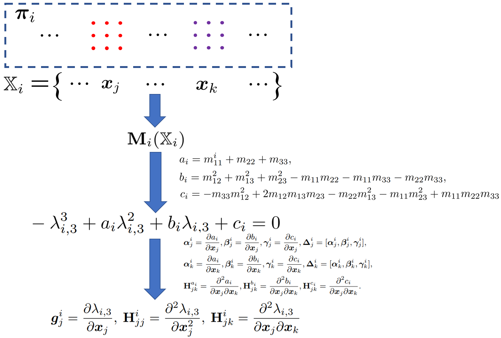
Refer to caption
Figure 7: Summary of our algorithm. 𝕏i\mathbb{X}_{i} is the set of poses which can see 𝝅i\bm{\pi}_{i}. Here 𝒙j∈𝕏i\bm{x}_{j}\in\mathbb{X}_{i} and 𝒙k∈𝕏i\bm{x}_{k}\in\mathbb{X}_{i}. The key point of our algorithm is to get 𝒈ji=∂λi,3∂𝒙j\bm{g}_{j}^{i}=\frac{\partial\lambda_{i,3}}{\partial\bm{x}_{j}}, 𝐇j​ji=∂2λi,3∂𝒙j2\mathbf{H}_{jj}^{i}=\frac{\partial^{2}\lambda_{i,3}}{\partial\bm{x}_{j}^{2}}, and 𝐇j​ki=∂2λi,3∂𝒙j​∂𝒙k\mathbf{H}_{jk}^{i}=\frac{\partial^{2}\lambda_{i,3}}{\partial\bm{x}_{j}\partial\bm{x}_{k}}. Theorem 1 provides their formulas. From Theorem 1, we know that the partial derivatives of aia_{i}, bib_{i}, and cic_{i} with respect to 𝒙j\bm{x}_{j} and 𝒙k\bm{x}_{k} in (23) are crucial. As aia_{i}, bib_{i}, and cic_{i} are polynomials with respect to me​fm_{ef} (e=1,2,3e=1,2,3 and f=1,2,3f=1,2,3), to get the partial derivatives of aia_{i}, bib_{i}, and cic_{i} with respect to 𝒙j\bm{x}_{j} and 𝒙k\bm{x}_{k}, we need to compute the partial derivatives of me​fm_{ef} with respect to 𝒙j\bm{x}_{j} and 𝒙k\bm{x}_{k}. Section 7.7 proves these partial derivatives of me​fm_{ef}.
Proof.

Expanding the definition of 𝚫ji\bm{\Delta}_{j}^{i} in (23), we have

𝚫ji=[∂ai∂xj​1∂bi∂xj​1∂ci∂xj​1∂ai∂xj​m∂bi∂xj​m∂ci∂xj​m∂ai∂xj​6∂bi∂xj​6∂ci∂xj​6]∈ℝ6×6\bm{\Delta}_{j}^{i}=\begin{bmatrix}\frac{\partial a_{i}}{\partial x_{j1}}&\frac{\partial b_{i}}{\partial x_{j1}}&\frac{\partial c_{i}}{\partial x_{j1}}\\ \vdots&\vdots&\vdots\\ \frac{\partial a_{i}}{\partial x_{jm}}&\frac{\partial b_{i}}{\partial x_{jm}}&\frac{\partial c_{i}}{\partial x_{jm}}\\ \vdots&\vdots&\vdots\\ \frac{\partial a_{i}}{\partial x_{j6}}&\frac{\partial b_{i}}{\partial x_{j6}}&\frac{\partial c_{i}}{\partial x_{j6}}\end{bmatrix}\in\mathbb{R}^{6\times 6} (45)

Substituting the definition of 𝜹j​mi\bm{\delta}_{jm}^{i} in (37) into (45), we can write 𝚫ji\bm{\Delta}_{j}^{i} as

𝚫ji=[𝜹j​1iT𝜹j​miT𝜹j​6iT]\bm{\Delta}_{j}^{i}=\begin{bmatrix}{\bm{\delta}_{j1}^{i}}^{T}\\ \vdots\\ {\bm{\delta}_{jm}^{i}}^{T}\\ \vdots\\ {\bm{\delta}_{j6}^{i}}^{T}\end{bmatrix} (46)

Assume xj​mx_{jm} is the mmth variable of 𝒙j\bm{x}_{j}. Then 𝒈ji\bm{g}_{j}^{i} can be written as

𝒈ji=∂λi,3∂𝒙j=[∂λi,3∂xj​1∂λi,3∂xj​m∂λi,3∂xj​6]∈ℝ6.\bm{g}_{j}^{i}=\frac{\partial\lambda_{i,3}}{\partial\bm{x}_{j}}=\begin{bmatrix}\frac{\partial\lambda_{i,3}}{\partial{x}_{j1}}\\ \vdots\\ \frac{\partial\lambda_{i,3}}{\partial{x}_{jm}}\\ \vdots\\ \frac{\partial\lambda_{i,3}}{\partial{x}_{j6}}\end{bmatrix}\in\mathbb{R}^{6}. (47)

Here ∂λi,3∂xj​m\frac{\partial\lambda_{i,3}}{\partial x_{jm}} is the mmth element of 𝒈ji\bm{g}_{j}^{i}. Substituting (46) into 𝒈ji\bm{g}_{j}^{i} in (24), we can obtain the formula of ∂λi,3∂xj​m\frac{\partial\lambda_{i,3}}{\partial x_{jm}} as

∂λi,3∂xj​m=−φi𝜹j​miT𝝌i=−φi𝜹j​mi⋅𝝌i.\frac{\partial\lambda_{i,3}}{\partial x_{jm}}=-\varphi_{i}{\bm{\delta}_{jm}^{i}}^{T}\bm{\chi}_{i}=-\varphi_{i}{\bm{\delta}_{jm}^{i}}\cdot\bm{\chi}_{i}. (48)

The above formula is what we proved in Lemma 1. Using Lemma 1, we known that the formula of 𝒈ji\bm{g}_{j}^{i} in (24) is correct.

Now we consider the Hessian matrix. According to the definitions of 𝜹k​ni\bm{\delta}_{kn}^{i}, 𝝌i\bm{\chi}_{i}, and 𝜹j​mi\bm{\delta}_{jm}^{i}, we have

𝜹k​ni=[∂ai∂xk​n∂bi∂xk​n∂ci∂xk​n],∂𝝌i∂xj,m=[2​λi,32​∂λi,3∂xj,m∂λi,3∂xj,m0],∂𝜹j​mi∂xk​n=[∂2ai∂xj​m​∂xk​n∂2bi∂xj​m​∂xk​n∂2ci∂xj​m​∂xk​n]\small\begin{split}\bm{\delta}_{kn}^{i}&=\begin{bmatrix}\frac{\partial a_{i}}{\partial x_{kn}}\\ \frac{\partial b_{i}}{\partial x_{kn}}\\ \frac{\partial c_{i}}{\partial x_{kn}}\end{bmatrix},\frac{\partial\bm{\chi}_{i}}{\partial x_{j,m}}=\begin{bmatrix}2\lambda_{i,3}^{2}\frac{\partial\lambda_{i,3}}{\partial x_{j,m}}\\ \frac{\partial\lambda_{i,3}}{\partial x_{j,m}}\\ 0\end{bmatrix},\frac{\partial\bm{\delta}_{jm}^{i}}{\partial x_{kn}}=\begin{bmatrix}\frac{\partial^{2}a_{i}}{\partial x_{jm}\partial x_{kn}}\\ \frac{\partial^{2}b_{i}}{\partial x_{jm}\partial x_{kn}}\\ \frac{\partial^{2}c_{i}}{\partial x_{jm}\partial x_{kn}}\end{bmatrix}\end{split} (49)

In addition, using the definition of φi\varphi_{i} in (21), we obtain

∂φi−1∂xk​m=𝝌i⋅∂𝜿i∂xk​m+𝜿i⋅∂𝝌i∂xk​m=2​λi,3​∂ai∂xk​n+∂bi∂xk​n+(2​a−6​λi,3)​∂λi,3∂xk​n\begin{split}\frac{\partial\varphi_{i}^{-1}}{\partial x_{km}}&=\bm{\chi}_{i}\cdot\frac{\partial\bm{\kappa}_{i}}{\partial x_{km}}+\bm{\kappa}_{i}\cdot\frac{\partial\bm{\chi}_{i}}{\partial x_{km}}\\ &=2\lambda_{i,3}\frac{\partial a_{i}}{\partial x_{kn}}+\frac{\partial b_{i}}{\partial x_{kn}}+\left(2a-6\lambda_{i,3}\right)\frac{\partial\lambda_{i,3}}{\partial x_{kn}}\end{split} (50)

Let us denote the entry in the mmth row and nnth column of 𝐇j​ki\mathbf{H}_{jk}^{i} as 𝐇j​ki​(m,n)\mathbf{H}_{jk}^{i}(m,n). Using the formula of 𝐇j​ki\mathbf{H}_{jk}^{i} in (24) and the variables in (49) and (50), we have

𝐇j​ki​(m,n)=−φi​∂λi,3∂xk​n​(2​λi,3​∂ai∂xj​m+∂bi∂xj​m)⏟φi​𝜹k​ni⋅∂𝝌i∂xj​m−φi​(λi,32​∂2ai∂xj​m​∂xk​n+λi,3​∂2bi∂xj​m​∂xk​n+∂2ci∂xj​m​∂xk​n)⏟φi​𝝌i⋅∂𝜹j​mi∂xk​n+φi​∂λi,3∂xj​m​(2​λi,3​∂ai∂xk​n+∂bi∂xk​n+(2​a−6​λi,3)​∂λi,3∂xk​n)⏟φi​∂λi,3∂xj​m​∂φi−1∂xk​m=−φi​(𝜹j​mi⋅∂𝝌i∂xk​n+𝝌i⋅∂𝜹j​mi∂xk​n−∂λi,3∂xj​m​∂φi−1∂xk​m)\small\begin{split}\mathbf{H}_{jk}^{i}(m,n)=&-\underbrace{\varphi_{i}\frac{\partial\lambda_{i,3}}{\partial x_{kn}}\left(2\lambda_{i,3}\frac{\partial a_{i}}{\partial x_{jm}}+\frac{\partial b_{i}}{\partial x_{jm}}\right)}_{\varphi_{i}\bm{\delta}_{kn}^{i}\cdot\frac{\partial\bm{\chi}_{i}}{\partial x_{jm}}}-\\ &\underbrace{\varphi_{i}\left(\lambda_{i,3}^{2}\frac{\partial^{2}a_{i}}{\partial x_{jm}\partial x_{kn}}+\lambda_{i,3}\frac{\partial^{2}b_{i}}{\partial x_{jm}\partial x_{kn}}+\frac{\partial^{2}c_{i}}{\partial x_{jm}\partial x_{kn}}\right)}_{\varphi_{i}\bm{\chi}_{i}\cdot\frac{\partial\bm{\delta}_{jm}^{i}}{\partial x_{kn}}}+\\ &\underbrace{\varphi_{i}\frac{\partial\lambda_{i,3}}{\partial x_{jm}}\left(2\lambda_{i,3}\frac{\partial a_{i}}{\partial x_{kn}}+\frac{\partial b_{i}}{\partial x_{kn}}+\left(2a-6\lambda_{i,3}\right)\frac{\partial\lambda_{i,3}}{\partial x_{kn}}\right)}_{\varphi_{i}\frac{\partial\lambda_{i,3}}{\partial x_{jm}}\frac{\partial\varphi_{i}^{-1}}{\partial x_{km}}}\\ =&-\varphi_{i}\left(\bm{\delta}_{jm}^{i}\cdot\frac{\partial\bm{\chi}_{i}}{\partial x_{kn}}+\bm{\chi}_{i}\cdot\frac{\partial\bm{\delta}_{jm}^{i}}{\partial x_{kn}}-\frac{\partial\lambda_{i,3}}{\partial x_{jm}}\frac{\partial\varphi_{i}^{-1}}{\partial x_{km}}\right)\end{split} (51)

On the other hand, we know

𝐇j​ki​(m,n)=∂2λi,3∂xj​m​∂xk​n.\mathbf{H}_{jk}^{i}(m,n)=\frac{\partial^{2}\lambda_{i,3}}{\partial x_{jm}\partial x_{kn}}. (52)

Comparing (22) and (51), we know that the formula of 𝐇j​ki\mathbf{H}_{jk}^{i} in (24) is correct. ∎

7.5 Proof of Lemma 3

Proof.

For j∈o​b​s​(𝝅i)j\in obs(\bm{\pi}_{i}) and k∈o​b​s​(𝝅i)k\in obs(\bm{\pi}_{i}), we take 1Ni​𝐓j​𝒑~i​j\frac{1}{N_{i}}\mathbf{T}_{j}\tilde{\bm{p}}_{ij} and 1Ni​𝐓k​𝒑~i​k\frac{1}{N_{i}}\mathbf{T}_{k}\tilde{\bm{p}}_{ik} out the summation. Then, we can write 𝒑¯i\bar{\bm{p}}_{i} as

𝒑¯i​(𝒙j,𝒙k)=𝐓j​1Ni​𝒑~i​j⏟𝒒i​j+𝐓k​1Ni​𝒑~i​k⏟𝒒i​k+1Ni​∑n∈𝕆j​k𝐓n​𝒑~i​n⏟𝒄i​j​k.=𝐓j​𝒒i​j+𝐓k​𝒒i​k+𝒄i​j​k.\begin{split}\bar{\bm{p}}_{i}(\bm{x}_{j},\bm{x}_{k})&=\mathbf{T}_{j}\underbrace{\frac{1}{N_{i}}\tilde{\bm{p}}_{ij}}_{\bm{q}_{ij}}+\mathbf{T}_{k}\underbrace{\frac{1}{N_{i}}\tilde{\bm{p}}_{ik}}_{\bm{q}_{ik}}+\underbrace{\frac{1}{N_{i}}\sum_{n\in\mathbb{O}_{jk}}\mathbf{T}_{n}\tilde{\bm{p}}_{in}}_{\bm{c}_{ijk}}.\\ &=\mathbf{T}_{j}\bm{q}_{ij}+\mathbf{T}_{k}\bm{q}_{ik}+\bm{c}_{ijk}.\end{split} (53)

For j∈o​b​s​(𝝅i)j\in obs(\bm{\pi}_{i}), we can write (53) as

𝒑¯i​(𝒙j,𝒙k)=𝐓j​𝒒i​j+𝐓k​𝒒i​k+𝒄i​j​k⏟𝒄i​j=𝐓j​𝒒i​j+𝒄i​j\begin{split}\bar{\bm{p}}_{i}(\bm{x}_{j},\bm{x}_{k})&=\mathbf{T}_{j}\bm{q}_{ij}+\underbrace{\mathbf{T}_{k}\bm{q}_{ik}+\bm{c}_{ijk}}_{\bm{c}_{ij}}\\ &=\mathbf{T}_{j}\bm{q}_{ij}+\bm{c}_{ij}\end{split} (54)

∎

7.6 Proof of Theorem 2

Proof.

Substituting (54) into (12) and using the formula of 𝐒i​j=𝐓j​𝐔𝐓jT\mathbf{S}_{ij}=\mathbf{T}_{j}\mathbf{U}\mathbf{T}_{j}^{T} in (13), we have

𝐌i​(𝒙i)=∑j∈o​b​s​(𝝅i)𝐒i​j−Ni​(𝐓j​𝒒i​j+𝒄i​j)​(𝐓j​𝒒i​j+𝒄i​j)T=𝐒i​j−𝐓j​(Ni​𝒒i​j​𝒒i​jT)​𝐓jT−𝐓j​(Nj​𝒒i​j​𝒄i​jT)⏟−𝐊ji−(Nj​𝒄i​j​𝒑i​jT)⏟(−𝐊ji)T​𝐓jT+∑n∈o​b​s​(𝝅i)n≠j𝐒i​n−Nj​𝒄i​j​𝒄i​jT⏟𝐂ji=𝐓j​𝐔i​j​𝐓jT−𝐓j​(Ni​𝒒i​j​𝒒i​jT)​𝐓jT+𝐓j​𝐊ji+(𝐊ji)T​𝐓jT+𝐂ji=𝐓j​(𝐔i​j−Nj​𝒒i​j​𝒒i​jT)⏟𝐐ji​𝐓jT+𝐓j​𝐊ji+(𝐊ji)T​𝐓jT+𝐂ji=𝐓j​𝐐ji​𝐓jT+𝐓j​𝐊ji+(𝐊ji)T​𝐓jT+𝐂ji\small\begin{split}\mathbf{M}_{i}(\bm{x}_{i})=&\sum_{j\in obs(\bm{\pi}_{i})}\mathbf{S}_{ij}-N_{i}(\mathbf{T}_{j}\bm{q}_{ij}+\bm{c}_{ij})(\mathbf{T}_{j}\bm{q}_{ij}+\bm{c}_{ij})^{T}\\ =&\mathbf{S}_{ij}-\mathbf{T}_{j}\left(N_{i}\bm{q}_{ij}\bm{q}_{ij}^{T}\right)\mathbf{T}_{j}^{T}-\mathbf{T}_{j}\underbrace{\left(N_{j}\bm{q}_{ij}\bm{c}_{ij}^{T}\right)}_{-\mathbf{K}_{j}^{i}}-\\ &\underbrace{\left(N_{j}\bm{c}_{ij}\bm{p}^{T}_{ij}\right)}_{\left(-\mathbf{K}_{j}^{i}\right)^{T}}\mathbf{T}_{j}^{T}+\underbrace{\sum_{\begin{subarray}{c}n\in obs(\bm{\pi}_{i})\\ n\neq j\end{subarray}}\mathbf{S}_{in}-N_{j}\bm{c}_{ij}\bm{c}_{ij}^{T}}_{\mathbf{C}_{j}^{i}}\\ =&\mathbf{T}_{j}\mathbf{U}_{ij}\mathbf{T}_{j}^{T}-\mathbf{T}_{j}\left(N_{i}\bm{q}_{ij}\bm{q}_{ij}^{T}\right)\mathbf{T}_{j}^{T}+\mathbf{T}_{j}\mathbf{K}_{j}^{i}+\left(\mathbf{K}_{j}^{i}\right)^{T}\mathbf{T}_{j}^{T}+\mathbf{C}_{j}^{i}\\ =&\mathbf{T}_{j}\underbrace{\left(\mathbf{U}_{ij}-N_{j}\bm{q}_{ij}\bm{q}_{ij}^{T}\right)}_{\mathbf{Q}_{j}^{i}}\mathbf{T}_{j}^{T}+\mathbf{T}_{j}\mathbf{K}_{j}^{i}+\left(\mathbf{K}_{j}^{i}\right)^{T}\mathbf{T}_{j}^{T}+\mathbf{C}_{j}^{i}\\ =&\mathbf{T}_{j}\mathbf{Q}_{j}^{i}\mathbf{T}_{j}^{T}+\mathbf{T}_{j}\mathbf{K}_{j}^{i}+(\mathbf{K}_{j}^{i})^{T}\mathbf{T}_{j}^{T}+\mathbf{C}_{j}^{i}\end{split}

Thus we get the formula of 𝐌i​(𝒙j)\mathbf{M}_{i}(\bm{x}_{j}) in (28). Now let us prove (29). Let us define

𝐄ji=𝐓j​𝒒i​j​(𝐓j​𝒒i​j+𝒄i​j​k)T𝐄ki=𝐓k​𝒒i​k​(𝐓k​𝒒i​k+𝒄i​j​k)T\begin{split}\mathbf{E}_{j}^{i}&=\mathbf{T}_{j}\bm{q}_{ij}\left(\mathbf{T}_{j}\bm{q}_{ij}+\bm{c}_{ijk}\right)^{T}\\ \mathbf{E}_{k}^{i}&=\mathbf{T}_{k}\bm{q}_{ik}\left(\mathbf{T}_{k}\bm{q}_{ik}+\bm{c}_{ijk}\right)^{T}\end{split} (55)

Substituting (53) into (12), we obtain

𝐌i​(𝒙j,𝒙k)=𝐓j​(−N​𝒒i​j​𝒒i​kT)⏟𝐎ji​𝐓kT+𝐓j​(−N​𝒒i​k​𝒒i​jT)⏟(𝐎ji)T​𝐓kT+∑j∈o​b​s​(𝝅i)𝐒i​j−Ni​(𝐄ji+𝐄ki+𝒄i​j​k​𝒑¯i​(𝒙j,𝒙k)T)⏟𝐂j​ki=𝐓j​𝐎j​ki​𝐓kT+𝐓k​(𝐎j​ki)T​𝐓jT+𝐂j​ki\begin{split}\mathbf{M}_{i}(\bm{x}_{j},\bm{x}_{k})=&\mathbf{T}_{j}\underbrace{\left(-N\bm{q}_{ij}\bm{q}_{ik}^{T}\right)}_{\mathbf{O}_{j}^{i}}\mathbf{T}_{k}^{T}+\mathbf{T}_{j}\underbrace{\left(-N\bm{q}_{ik}\bm{q}_{ij}^{T}\right)}_{\left(\mathbf{O}_{j}^{i}\right)^{T}}\mathbf{T}_{k}^{T}+\\ &\underbrace{\sum_{j\in obs(\bm{\pi}_{i})}\mathbf{S}_{ij}-N_{i}\left(\mathbf{E}_{j}^{i}+\mathbf{E}_{k}^{i}+\bm{c}_{ijk}\bar{\bm{p}}_{i}(\bm{x}_{j},\bm{x}_{k})^{T}\right)}_{\mathbf{C}_{jk}^{i}}\\ =&\mathbf{T}_{j}\mathbf{O}_{jk}^{i}\mathbf{T}_{k}^{T}+\mathbf{T}_{k}{(\mathbf{O}_{jk}^{i})}^{T}\mathbf{T}_{j}^{T}+\mathbf{C}_{jk}^{i}\end{split} (56)

Thus we get the formula of 𝐌i​(𝒙j,𝒙k)\mathbf{M}_{i}(\bm{x}_{j},\bm{x}_{k}) in (29). ∎

7.7 Partial Derivatives of Entries in Mi

As illustrated in Fig. 7, the derivatives of aia_{i}, bib_{i} and cic_{i} in (23) are the crux to get 𝒈ji\bm{g}_{j}^{i}, 𝐇j​ji\mathbf{H}_{jj}^{i}, and 𝐇j​ki\mathbf{H}_{jk}^{i}. The aia_{i}, bib_{i} and cic_{i} in (19) are first-, second-, and third-order polynomials with respect to the elements in 𝐌i\mathbf{M}_{i}, respectively. Let us denote the eeth row and ffth column entry of 𝐌i\mathbf{M}_{i} as me​fm_{ef}. According to the chain rule in calculus, to compute the partial derivatives in (23), we have to calculate

∂me​f∂𝒙j,∂2me​f∂𝒙j2,and​∂2me​f∂𝒙j​∂𝒙k.\frac{\partial m_{ef}}{\partial\bm{x}_{j}},\frac{\partial^{2}m_{ef}}{\partial\bm{x}_{j}^{2}},\ \text{and}\ \frac{\partial^{2}m_{ef}}{\partial\bm{x}_{j}\partial\bm{x}_{k}}. (57)

From our paper, we know that we only need to compute their value at 𝒙0=[0;0;0;0;0;0]\bm{x}_{0}=[0;0;0;0;0;0]. Assume qe​f{q}_{ef}, ke​f{k}_{ef}, and oe​fo_{ef} are the eeth row and ffth column entries of 𝐐ji\mathbf{Q}_{j}^{i}, 𝐊ji\mathbf{K}_{j}^{i}, and 𝐎j​ki\mathbf{O}_{jk}^{i}, respectively. Then, the values of ∂me​f∂𝒙j\frac{\partial m_{ef}}{\partial\bm{x}_{j}}, ∂2me​f∂𝒙j​∂𝒙k\frac{\partial^{2}m_{ef}}{\partial\bm{x}_{j}\partial\bm{x}_{k}}, and ∂2me​f∂𝒙j2\frac{\partial^{2}m_{ef}}{\partial\bm{x}_{j}^{2}} at 𝒙0\bm{x}_{0} have the forms in Table 1, Table 2, and Table 3, respectively.

∂m11∂𝒙j|𝒙j=𝒙0=[0−2​k31−2​q132​k21+2​q12−4​k32−4​q232​k22−2​k33+2​q22−2​q334​k23+4​q23]\left.\frac{\partial m_{11}}{\partial\bm{x}_{j}}\right|_{\bm{x}_{j}=\bm{x}_{0}}=\begin{bmatrix}0\\ -2k_{31}-2q_{13}\\ 2k_{21}+2q_{12}\\ -4k_{32}-4q_{23}\\ 2k_{22}-2k_{33}+2q_{22}-2q_{33}\\ 4k_{23}+4q_{23}\\ \end{bmatrix} ∂m12∂𝒙j|𝒙j=𝒙0=[4​k31+4​q132​k32+2​q232​k33−2​k11−2​q11+2​q330−2​k12−2​q12−4​k13−4​q13]\left.\frac{\partial m_{12}}{\partial\bm{x}_{j}}\right|_{\bm{x}_{j}=\bm{x}_{0}}=\begin{bmatrix}4k_{31}+4q_{13}\\ 2k_{32}+2q_{23}\\ 2k_{33}-2k_{11}-2q_{11}+2q_{33}\\ 0\\ -2k_{12}-2q_{12}\\ -4k_{13}-4q_{13}\\ \end{bmatrix}
∂m13∂𝒙j|𝒙j=𝒙0=[−4​k21−4​q122​k11−2​k22+2​q11−2​q22−2​k23−2​q234​k12+4​q122​k13+2​q130]\left.\frac{\partial m_{13}}{\partial\bm{x}_{j}}\right|_{\bm{x}_{j}=\bm{x}_{0}}=\begin{bmatrix}-4k_{21}-4q_{12}\\ 2k_{11}-2k_{22}+2q_{11}-2q_{22}\\ -2k_{23}-2q_{23}\\ 4k_{12}+4q_{12}\\ 2k_{13}+2q_{13}\\ 0\\ \end{bmatrix} ∂m22∂𝒙j|𝒙j=𝒙0=[2​k41+2​q14k42+q24k43+q34000]\left.\frac{\partial m_{22}}{\partial\bm{x}_{j}}\right|_{\bm{x}_{j}=\bm{x}_{0}}=\begin{bmatrix}2k_{41}+2q_{14}\\ k_{42}+q_{24}\\ k_{43}+q_{34}\\ 0\\ 0\\ 0\\ \end{bmatrix}
∂m23∂𝒙j|𝒙j=𝒙0=[0k41+q1402​k42+2​q24k43+q340]\left.\frac{\partial m_{23}}{\partial\bm{x}_{j}}\right|_{\bm{x}_{j}=\bm{x}_{0}}=\begin{bmatrix}0\\ k_{41}+q_{14}\\ 0\\ 2k_{42}+2q_{24}\\ k_{43}+q_{34}\\ 0\end{bmatrix} ∂m33∂𝒙j|𝒙j=𝒙0=[00k41+q140k42+q242​k43+2​q34]\left.\frac{\partial m_{33}}{\partial\bm{x}_{j}}\right|_{\bm{x}_{j}=\bm{x}_{0}}=\begin{bmatrix}0\\ 0\\ k_{41}+q_{14}\\ 0\\ k_{42}+q_{24}\\ 2k_{43}+2q_{34}\end{bmatrix}
Table 1: ∂me​f∂𝒙j\frac{\partial m_{ef}}{\partial\bm{x}_{j}} at 𝒙j=𝒙0\bm{x}_{j}=\bm{x}_{0}.
∂2m11∂𝒙j​∂𝒙k|𝒙j=𝒙0𝒙k=𝒙0=[00000008​o33−8​o324​o34000−8​o238​o22−4​o240004​o43−4​o422​o4400000000000000]\left.\frac{\partial^{2}m_{11}}{\partial\bm{x}_{j}\partial\bm{x}_{k}}\right|_{\begin{subarray}{c}\bm{x}_{j}=\bm{x}_{0}\\ \bm{x}_{k}=\bm{x}_{0}\end{subarray}}=\begin{bmatrix}0&0&0&0&0&0\\ 0&8o_{33}&-8o_{32}&4o_{34}&0&0\\ 0&-8o_{23}&8o_{22}&-4o_{24}&0&0\\ 0&4o_{43}&-4o_{42}&2o_{44}&0&0\\ 0&0&0&0&0&0\\ 0&0&0&0&0&0\\ \end{bmatrix} ∂2m13∂𝒙j​∂𝒙k|𝒙j=𝒙0𝒙k=𝒙0=[04​o23−4​o222​o24004​o32−4​o13−4​o314​o12−2​o1402​o34−4​o224​o21000−2​o242​o42−2​o41000o4400000002​o43−2​o42o4400]\left.\frac{\partial^{2}m_{13}}{\partial\bm{x}_{j}\partial\bm{x}_{k}}\right|_{\begin{subarray}{c}\bm{x}_{j}=\bm{x}_{0}\\ \bm{x}_{k}=\bm{x}_{0}\end{subarray}}=\begin{bmatrix}0&4o_{23}&-4o_{22}&2o_{24}&0&0\\ 4o_{32}&-4o_{13}-4o_{31}&4o_{12}&-2o_{14}&0&2o_{34}\\ -4o_{22}&4o_{21}&0&0&0&-2o_{24}\\ 2o_{42}&-2o_{41}&0&0&0&o_{44}\\ 0&0&0&0&0&0\\ 0&2o_{43}&-2o_{42}&o_{44}&0&0\\ \end{bmatrix}
∂2m22∂𝒙j​∂𝒙k|𝒙j=𝒙0𝒙k=𝒙0=[8​o330−8​o310−4​o340000000−8​o1308​o1104​o140000000−4​o4304​o4102​o440000000]\left.\frac{\partial^{2}m_{22}}{\partial\bm{x}_{j}\partial\bm{x}_{k}}\right|_{\begin{subarray}{c}\bm{x}_{j}=\bm{x}_{0}\\ \bm{x}_{k}=\bm{x}_{0}\end{subarray}}=\begin{bmatrix}8o_{33}&0&-8o_{31}&0&-4o_{34}&0\\ 0&0&0&0&0&0\\ -8o_{13}&0&8o_{11}&0&4o_{14}&0\\ 0&0&0&0&0&0\\ -4o_{43}&0&4o_{41}&0&2o_{44}&0\\ 0&0&0&0&0&0\\ \end{bmatrix} ∂2m12∂𝒙j​∂𝒙k|𝒙j=𝒙0𝒙k=𝒙0=[0−4​o334​o32−2​o3400−4​o3304​o3102​o3404​o234​o13−4​o12−4​o212​o14−2​o240−2​o4302​o410o44002​o43−2​o42o4400000000]\left.\frac{\partial^{2}m_{12}}{\partial\bm{x}_{j}\partial\bm{x}_{k}}\right|_{\begin{subarray}{c}\bm{x}_{j}=\bm{x}_{0}\\ \bm{x}_{k}=\bm{x}_{0}\end{subarray}}=\begin{bmatrix}0&-4o_{33}&4o_{32}&-2o_{34}&0&0\\ -4o_{33}&0&4o_{31}&0&2o_{34}&0\\ 4o_{23}&4o_{13}&-4o_{12}-4o_{21}&2o_{14}&-2o_{24}&0\\ -2o_{43}&0&2o_{41}&0&o_{44}&0\\ 0&2o_{43}&-2o_{42}&o_{44}&0&0\\ 0&0&0&0&0&0\\ \end{bmatrix}
∂2m33∂𝒙j​∂𝒙k|𝒙j=𝒙0𝒙k=𝒙0=[8​o22−8​o210004​o24−8​o128​o11000−4​o140000000000000000004​o42−4​o410002​o44]\left.\frac{\partial^{2}m_{33}}{\partial\bm{x}_{j}\partial\bm{x}_{k}}\right|_{\begin{subarray}{c}\bm{x}_{j}=\bm{x}_{0}\\ \bm{x}_{k}=\bm{x}_{0}\end{subarray}}=\begin{bmatrix}8o_{22}&-8o_{21}&0&0&0&4o_{24}\\ -8o_{12}&8o_{11}&0&0&0&-4o_{14}\\ 0&0&0&0&0&0\\ 0&0&0&0&0&0\\ 0&0&0&0&0&0\\ 4o_{42}&-4o_{41}&0&0&0&2o_{44}\\ \end{bmatrix} ∂2m23∂𝒙j​∂𝒙k|𝒙j=𝒙0𝒙k=𝒙0=[−4​o23−4​o324​o314​o2102​o24−2​o344​o130−4​o110−2​o1404​o12−4​o110002​o140000002​o42−2​o41000o44−2​o4302​o410o440]\left.\frac{\partial^{2}m_{23}}{\partial\bm{x}_{j}\partial\bm{x}_{k}}\right|_{\begin{subarray}{c}\bm{x}_{j}=\bm{x}_{0}\\ \bm{x}_{k}=\bm{x}_{0}\end{subarray}}=\begin{bmatrix}-4o_{23}-4o_{32}&4o_{31}&4o_{21}&0&2o_{24}&-2o_{34}\\ 4o_{13}&0&-4o_{11}&0&-2o_{14}&0\\ 4o_{12}&-4o_{11}&0&0&0&2o_{14}\\ 0&0&0&0&0&0\\ 2o_{42}&-2o_{41}&0&0&0&o_{44}\\ -2o_{43}&0&2o_{41}&0&o_{44}&0\\ \end{bmatrix}
Table 2: ∂2me​f∂𝒙j​∂𝒙k\frac{\partial^{2}m_{ef}}{\partial\bm{x}_{j}\partial\bm{x}_{k}} at 𝒙j=𝒙0\bm{x}_{j}=\bm{x}_{0} and 𝒙k=𝒙0\bm{x}_{k}=\bm{x}_{0}.
∂2m11∂𝒙j2|𝒙j=𝒙0=[04​k21+4​q124​k31+4​q130004​k21+4​q128​q33−8​q11−8​k11−8​q234​q34004​k31+4​q13−8​q238​q22−8​q11−8​k11−4​q240004​q34−4​q242​q4400000000000000]\left.\frac{\partial^{2}m_{11}}{\partial\bm{x}_{j}^{2}}\right|_{\bm{x}_{j}=\bm{x}_{0}}=\begin{bmatrix}0&4k_{21}+4q_{12}&4k_{31}+4q_{13}&0&0&0\\ 4k_{21}+4q_{12}&8q_{33}-8q_{11}-8k_{11}&-8q_{23}&4q_{34}&0&0\\ 4k_{31}+4q_{13}&-8q_{23}&8q_{22}-8q_{11}-8k_{11}&-4q_{24}&0&0\\ 0&4q_{34}&-4q_{24}&2q_{44}&0&0\\ 0&0&0&0&0&0\\ 0&0&0&0&0&0\end{bmatrix}
∂2m12∂𝒙j2|𝒙j=𝒙0=[−4​k21−4​q122​k11+2​k22+2​q11+2​q22−4​q332​k32+6​q23−2​q34002​k11+2​k22+2​q11+2​q22−4​q33−4​k12−4​q122​k31+6​q1302​q3402​k32+6​q232​k31+6​q13−4​k12−4​k21−16​q122​q14−2​q240−2​q3402​q14,0q44,002​q34−2​q24q4400000000]\left.\frac{\partial^{2}m_{12}}{\partial\bm{x}_{j}^{2}}\right|_{\bm{x}_{j}=\bm{x}_{0}}=\begin{bmatrix}-4k_{21}-4q_{12}&2k_{11}+2k_{22}+2q_{11}+2q_{22}-4q_{33}&2k_{32}+6q_{23}&-2q_{34}&0&0\\ 2k_{11}+2k_{22}+2q_{11}+2q_{22}-4q_{33}&-4k_{12}-4q_{12}&2k_{31}+6q_{13}&0&2q_{34}&0\\ 2k_{32}+6q_{23}&2k_{31}+6q_{13}&-4k_{12}-4k_{21}-16q_{12}&2q_{14}&-2q_{24}&0\\ -2q_{34}&0&2q_{14},0&q_{44},0\\ 0&2q_{34}&-2q_{24}&q_{44}&0&0\\ 0&0&0&0&0&0\\ \end{bmatrix}
∂2m13∂𝒙j2|𝒙j=𝒙0=[−4​k31−4​q132​k23+6​q232​k11+2​k33+2​q11−4​q22+2​q332​q24002​k23+6​q23−4​k13−4​k31−16​q132​k21+6​q12−2​q1402​q342​k11+2​k33+2​q11−4​q22+2​q332​k21+6​q12−4​k13−4​q1300−2​q242​q24−2​q14000q4400000002​q34−2​q24q4400]\left.\frac{\partial^{2}m_{13}}{\partial\bm{x}_{j}^{2}}\right|_{\bm{x}_{j}=\bm{x}_{0}}=\begin{bmatrix}-4k_{31}-4q_{13}&2k_{23}+6q_{23}&2k_{11}+2k_{33}+2q_{11}-4q_{22}+2q_{33}&2q_{24}&0&0\\ 2k_{23}+6q_{23}&-4k_{13}-4k_{31}-16q_{13}&2k_{21}+6q_{12}&-2q_{14}&0&2q_{34}\\ 2k_{11}+2k_{33}+2q_{11}-4q_{22}+2q_{33}&2k_{21}+6q_{12}&-4k_{13}-4q_{13}&0&0&-2q_{24}\\ 2q_{24}&-2q_{14}&0&0&0&q_{44}\\ 0&0&0&0&0&0\\ 0&2q_{34}&-2q_{24}&q_{44}&0&0\\ \end{bmatrix}
∂2m22∂𝒙j2|𝒙j=𝒙0=[8​q33−8​q22−8​k224​k12+4​q12−8​q130−4​q3404​k12+4​q1204​k32+4​q23000−8​q134​k32+4​q238​q11−8​k22−8​q2204​q140000000−4​q3404​q1402​q440000000]\left.\frac{\partial^{2}m_{22}}{\partial\bm{x}_{j}^{2}}\right|_{\bm{x}_{j}=\bm{x}_{0}}=\begin{bmatrix}8q_{33}-8q_{22}-8k_{22}&4k_{12}+4q_{12}&-8q_{13}&0&-4q_{34}&0\\ 4k_{12}+4q_{12}&0&4k_{32}+4q_{23}&0&0&0\\ -8q_{13}&4k_{32}+4q_{23}&8q_{11}-8k_{22}-8q_{22}&0&4q_{14}&0\\ 0&0&0&0&0&0\\ -4q_{34}&0&4q_{14}&0&2q_{44}&0\\ 0&0&0&0&0&0\\ \end{bmatrix}
∂2m23∂𝒙j2|𝒙j=𝒙0=[−4​k23−4​k32−16​q232​k13+6​q132​k12+6​q1202​q24−2​q342​k13+6​q13−4​k32−4​q232​k22+2​k33−4​q11+2​q22+2​q330−2​q1402​k12+6​q122​k22+2​k33−4​q11+2​q22+2​q33−4​k23−4​q23002​q14​10000002​q24−2​q14000q44−2​q3402​q140q440]\left.\frac{\partial^{2}m_{23}}{\partial\bm{x}_{j}^{2}}\right|_{\bm{x}_{j}=\bm{x}_{0}}=\begin{bmatrix}-4k_{23}-4k_{32}-16q_{23}&2k_{13}+6q_{13}&2k_{12}+6q_{12}&0&2q_{24}&-2q_{34}\\ 2k_{13}+6q_{13}&-4k_{32}-4q_{23}&2k_{22}+2k_{33}-4q_{11}+2q_{22}+2q_{33}&0&-2q_{14}&0\\ 2k_{12}+6q_{12}&2k_{22}+2k_{33}-4q_{11}+2q_{22}+2q_{33}&-4k_{23}-4q_{23}&0&0&2q_{14}1\\ 0&0&0&0&0&0\\ 2q_{24}&-2q_{14}&0&0&0&q_{44}\\ -2q_{34}&0&2q_{14}&0&q_{44}&0\\ \end{bmatrix}
∂2m33∂𝒙j2|𝒙j=𝒙0=[8​q22−8​k33−8​q33−8​q124​k13+4​q13004​q24−8​q128​q11−8​k33−8​q334​k23+4​q2300−4​q144​k13+4​q134​k23+4​q2300000000000000004​q24−4​q140002​q44]\left.\frac{\partial^{2}m_{33}}{\partial\bm{x}_{j}^{2}}\right|_{\bm{x}_{j}=\bm{x}_{0}}=\begin{bmatrix}8q_{22}-8k_{33}-8q_{33}&-8q_{12}&4k_{13}+4q_{13}&0&0&4q_{24}\\ -8q_{12}&8q_{11}-8k_{33}-8q_{33}&4k_{23}+4q_{23}&0&0&-4q_{14}\\ 4k_{13}+4q_{13}&4k_{23}+4q_{23}&0&0&0&0\\ 0&0&0&0&0&0\\ 0&0&0&0&0&0\\ 4q_{24}&-4q_{14}&0&0&0&2q_{44}\\ \end{bmatrix}
Table 3: ∂2me​f∂𝒙j2\frac{\partial^{2}m_{ef}}{\partial\bm{x}_{j}^{2}} at 𝒙j=𝒙0\bm{x}_{j}=\bm{x}_{0}.

References

  • (1) Implicit Funtion Theorem. https://en.wikipedia.org/wiki/Implicit_function_theorem.
  • (2) Sameer Agarwal, Yasutaka Furukawa, Noah Snavely, Ian Simon, Brian Curless, Steven M Seitz, and Richard Szeliski. Building rome in a day. Communications of the ACM, 54(10):105–112, 2011.
  • (3) Sameer Agarwal, Keir Mierle, and The Ceres Solver Team. Ceres Solver, 3 2022.
  • (4) Sameer Agarwal, Noah Snavely, Steven M Seitz, and Richard Szeliski. Bundle adjustment in the large. In European conference on computer vision, pages 29–42. Springer, 2010.
  • (5) Alex M Andrew. Multiple view geometry in computer vision. Kybernetes, 2001.
  • (6) Carlos Campos, Richard Elvira, Juan J Gómez Rodríguez, José MM Montiel, and Juan D Tardós. Orb-slam3: An accurate open-source library for visual, visual–inertial, and multimap slam. IEEE Transactions on Robotics, 2021.
  • (7) Danpeng Chen, Shuai Wang, Weijian Xie, Shangjin Zhai, Nan Wang, Hujun Bao, and Guofeng Zhang. Vip-slam: An efficient tightly-coupled rgb-d visual inertial planar slam. In 2022 International Conference on Robotics and Automation (ICRA), pages 5615–5621. IEEE, 2022.
  • (8) Nikolaus Demmel, David Schubert, Christiane Sommer, Daniel Cremers, and Vladyslav Usenko. Square root marginalization for sliding-window bundle adjustment. In Proceedings of the IEEE/CVF International Conference on Computer Vision, pages 13260–13268, 2021.
  • (9) Nikolaus Demmel, Christiane Sommer, Daniel Cremers, and Vladyslav Usenko. Square root bundle adjustment for large-scale reconstruction. In Proceedings of the IEEE/CVF Conference on Computer Vision and Pattern Recognition, pages 11723–11732, 2021.
  • (10) Hakim Elchaoui Elghor, David Roussel, Fakhreddine Ababsa, and El Houssine Bouyakhf. Planes detection for robust localization and mapping in rgb-d slam systems. In 2015 International Conference on 3D Vision, pages 452–459. IEEE, 2015.
  • (11) Gonzalo Ferrer. Eigen-factors: Plane estimation for multi-frame and time-continuous point cloud alignment. In 2019 IEEE/RSJ International Conference on Intelligent Robots and Systems (IROS), pages 1278–1284. IEEE, 2019.
  • (12) Joel A Hesch and Stergios I Roumeliotis. A direct least-squares (dls) method for pnp. In 2011 International Conference on Computer Vision, pages 383–390. IEEE, 2011.
  • (13) Ming Hsiao, Eric Westman, Guofeng Zhang, and Michael Kaess. Keyframe-based dense planar slam. In 2017 IEEE International Conference on Robotics and Automation (ICRA), pages 5110–5117. IEEE, 2017.
  • (14) Michael Kaess. Simultaneous localization and mapping with infinite planes. In 2015 IEEE International Conference on Robotics and Automation (ICRA), pages 4605–4611. IEEE, 2015.
  • (15) Pyojin Kim, Brian Coltin, and H Jin Kim. Linear rgb-d slam for planar environments. In Proceedings of the European Conference on Computer Vision (ECCV), pages 333–348, 2018.
  • (16) Steven George Krantz and Harold R Parks. The implicit function theorem: history, theory, and applications. Springer Science & Business Media, 2002.
  • (17) Zheng Liu and Fu Zhang. BALM: Bundle Adjustment for LiDAR Mapping. IEEE Robotics and Automation Letters, 6(2):3184–3191, 2021.
  • (18) Jorge J Moré. The levenberg-marquardt algorithm: implementation and theory. In Numerical analysis, pages 105–116. Springer, 1978.
  • (19) Raul Mur-Artal, Jose Maria Martinez Montiel, and Juan D Tardos. Orb-slam: a versatile and accurate monocular slam system. IEEE transactions on robotics, 31(5):1147–1163, 2015.
  • (20) Johannes L Schonberger and Jan-Michael Frahm. Structure-from-motion revisited. In Proceedings of the IEEE conference on computer vision and pattern recognition, pages 4104–4113, 2016.
  • (21) Bill Triggs, Philip F McLauchlan, Richard I Hartley, and Andrew W Fitzgibbon. Bundle adjustment—a modern synthesis. In International workshop on vision algorithms, pages 298–372. Springer, 1999.
  • (22) Ji Zhang and Sanjiv Singh. Loam: Lidar odometry and mapping in real-time. In Robotics: Science and Systems, volume 2, 2014.
  • (23) Lipu Zhou, Guoquan Huang, Yinian Mao, Jincheng Yu, Shengze Wang, and Michael Kaess. Plc-lislam: Lidar slam with planes, lines and cylinders. IEEE Robotics and Automation Letters, 2022.
  • (24) Lipu Zhou, Daniel Koppel, Hul Ju, Frank Steinbruecker, and Michael Kaess. An efficient planar bundle adjustment algorithm. In 2020 IEEE International Symposium on Mixed and Augmented Reality (ISMAR), pages 136–145, 2020.
  • (25) Lipu Zhou, Daniel Koppel, and Michael Kaess. Lidar slam with plane adjustment for indoor environment. IEEE Robotics and Automation Letters, 6(4):7073–7080, 2021.
  • (26) Lei Zhou, Zixin Luo, Mingmin Zhen, Tianwei Shen, Shiwei Li, Zhuofei Huang, Tian Fang, and Long Quan. Stochastic bundle adjustment for efficient and scalable 3d reconstruction. In European Conference on Computer Vision, pages 364–379. Springer, 2020.
  • (27) Lipu Zhou, Shengze Wang, and Michael Kaess. π\pi-lsam: Lidar smoothing and mapping with planes. In 2021 IEEE International Conference on Robotics and Automation (ICRA), pages 5751–5757. IEEE, 2021.