Place Recognition under Occlusion and Changing Appearance via Disentangled Representations
Abstract
Place recognition is a critical and challenging task for mobile robots, aiming to retrieve an image captured at the same place as a query image from a database. Existing methods tend to fail while robots move autonomously under occlusion (e.g., car, bus, truck) and changing appearance (e.g., illumination changes, seasonal variation). Because they encode the image into only one code, entangling place features with appearance and occlusion features. To overcome this limitation, we propose PROCA, an unsupervised approach to decompose the image representation into three codes: a place code used as a descriptor to retrieve images, an appearance code that captures appearance properties, and an occlusion code that encodes occlusion content. Extensive experiments show that our model outperforms the state-of-the-art methods. Our code and data are available at https://github.com/rover-xingyu/PROCA.
I Introduction
Many problems in the localization of mobile robot focus on recognizing the place, including detecting the loop closure for Simultaneous Localization and Mapping (SLAM) and finding the initial pose for finer 6-DoF pose regression. Due to the properties of low cost, high resolution, and rich color information of cameras, visual place recognition has received extensive concern. For a query image, the goal is to retrieve an image corresponding to the same place from a database of geo-tagged images and approximate the pose of the retrieved image as the query’s pose.
The query and database images are taken under various occlusion and appearance conditions in many scenarios. For example, changing lighting and seasons lead to appearance variation, and dynamic objects contribute towards occlusion, like cars, buses and trucks around robots. Unfortunately, existing techniques generally encode an image into only one code, entangling place features with appearance and occlusion features. As a result, they fail to retrieve the correct images from a database. Some approaches disentangle content and appearance features, but are still affected by dynamic objects.
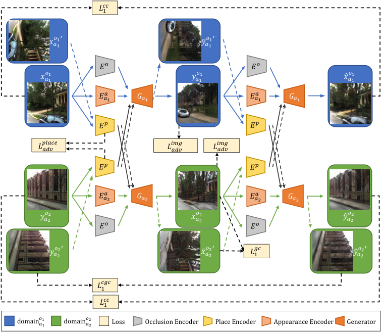
In this paper, we propose an unsupervised disentangled representation framework (Figure 1) for Place Recognition under Occlusion and Changing Appearance (PROCA). Our framework makes several assumptions. Firstly we assume that the latent space of an image can be decomposed into a place space, an appearance space and an occlusion space, as shown in Figure 2d. We further postulate that images in different domains share a common place space and a common occlusion space but not the appearance space. Because the aligned training image pairs are either difficult to collect (e.g., tuples of images depicting the same place under different conditions) or do not exist (e.g., images taken in the identical position under different conditions), we use the unsupervised image-to-image translation task as an auxiliary supervision. To translate an image to the target domain, we recombine its place code with an appearance code and an occlusion code from the target domain. During translation, the place code encodes the information that should be preserved, while the appearance code and occlusion code represent the remaining variables that are not contained in the input image.
We disentangle the representations by using a place adversarial loss to encourage the place code not to take domain-specific cues (e.g., edges of buildings), an appearance adversarial loss to facilitate the appearance code to carry appearance properties (e.g., sunlight intensity), an occlusion adversarial loss to stimulate the occlusion code to carry occlusion content (e.g., edges of cars). To tackle the unpaired problem, we first perform a cross-domain mapping to translate the image to another domain by swapping the place codes from unpaired images. We then reconstruct the original image pair by using cross-domain mapping again. Finally, we enforce the consistency between the original and the reconstructed images by leveraging a cross-cycle consistency loss. Moreover, we propose a geometry consistency loss and a cross-cycle geometry consistency loss to further separate the place code and the occlusion code, which is constructed by applying the cross-domain mapping to the counterpart image pair transformed by our predefined geometric transformation. At test time, we use the disentangled place code to retrieve an image corresponding to the same place from a pre-encoded database.
Extensive experiments demonstrate the effectiveness of our method in handling occlusion and changing appearance and the superiority in localization accuracy compared with state-of-the-art approaches.
II RELATED WORKS
II-A Image-to-Image Translation
Image-to-Image translation aims to learn the mapping from a source image domain to a target image domain. Introduced by Isola et al., Pix2pix [1] proposes the first unified framework for image-to-image translation based on conditional generative adversarial networks, using manually labeled image pairs. To train with unpaired data, the CycleGAN [2] schemes leverage cycle-consistency to regularize the training, which enforces that if we translate an image to the target domain and back, we should reconstruct the original image, as shown in Figure 2a. UNIT [3] and ComboGAN [4] further assume a shared latent space such that corresponding images in two domains are mapped to the same latent code, as illustrated in Figure 2b,
However, a summer scene could have diverse possible appearances during winter due to climate, timing, lighting, etc. For example, a summer landscape of lush greenery may become snow-covered or just leafless in winter. But supposed to enforce the reconstructed image to be the same as the original image by cycle-consistency constraint, the latent code will be entangled with appearance properties, which hampers the place recognition task. Unlike existing works, our method enables image-to-image translation with disentangled representations.

II-B Disentangled Representations
Learning disentangled representation refers to modeling the factors of data variations. Previous works leverage labeled data to factorize representations into class-related and class-independent components [5, 6, 7]. Recently, numerous unsupervised methods have been developed [8, 9, 10] to learn disentangled representations. As shown in Figure 2c, DRIT [9] and MUNIT [10] separate appearance and content components with adversarial and reconstruction objectives. They define ”content” as the underlying spatial structure and ”appearance” as the rendering of the structure.
However, a place could have many possible contents due to the occlusion caused by dynamic objects such as cars, buses and trucks. It is necessary for us to disentangle place content from occlusion content. In our setting, we disentangle an image into place, appearance and occlusion representations to facilitate learning place descriptors to retrieve images.
II-C Place Recognition and Localization
Place recognition tackles retrieving the image taken from the same place for a query image, usually used as a key module for the localization pipelines of mobile robots. Typical place recognition includes feature extraction and matching, optionally followed by sequence fusion [11, 12] to reduce the false positive rates, among which this paper focuses on the first part.
Conventional methods design features [13, 14, 15], or statistics of features as global descriptors [16, 17, 18, 19] to handle a fraction of illumination variation. However, they have been shown to be heavily affected by domain shifts such as weather, season and occlusion [20].
To close the domain gap, methods [21, 22] perform image translation from a source domain(e.g., night) to a target domain (e.g., day) and retrieve the output image through conventional descriptors. However, the retrieval effectiveness of these two-stage methods depends on the quality of translated image, which degrades their generalization ability.
By contrast, retrieval with latent features has the advantages of direct, low-cost and efficient learning. Methods [23, 24] are proposed to learn the domain-invariant representation via a ComboGAN-like [4] architecture. However, based on cycle-consistency constraints, they still try to translate and reconstruct the image from only one content code, which entangles the content code with appearance properties. Tang et al. [25] propose to use adversarial features disentanglement directly on the latent code to separate content and appearance. Nevertheless, the method is yet hampered by occlusion content from dynamic objects, while ours is not.
III PROPOSED METHOD
We propose to learn disentangled representations with the help of image-to-image translation. Given unpaired images and in two visual domains , e.g., winter with occlusion , and , e.g., summer without occlusion . As illustrated in Figure 1, our framework consists of a shared place encoder , a shared occlusion encoder , two appearance encoders , two generators , four discriminators , two for appearance and the others for occlusion, and a place discriminator . Taking domain as an example, the place encoder maps images onto a shared, domain-invariant place space , the occlusion encoder maps images onto a shared occlusion space , and the appearance encoder maps images onto a domain-specific appearance space . The generator synthesizes images conditioned on place, occlusion and appearance codes . The discriminator and aim to discriminate between real and translated images in the domain and , respectively. In addition, the place discriminator is trained to distinguish the place codes extracted from two domains.
III-A Cross-cycle Consistency Constraint
Thanks to the disentangled representations, we can perform image-to-image translation by combining a place code from a given image with an occlusion code and an appearance code from an image of the target domain. However, training with unpaired images is inherently ill-posed and requires additional constraints. Inspired by recent works [9, 26] that exploit the disentangled content and appearance codes for cyclic reconstruction, we propose a modified cross-cycle consistency loss to regularize training.
Given unpaired images and , we encode them into:
| (1) | ||||
We then perform the first translation by swapping the place representation to generate translated images , where and .
| (2) |
Next, we encode the translated images and into and , and perform the second translation by swapping the place representation again to generate reconstructed images .
| (3) |
Here we assume that the reconstructed images should be the same as the original images, and the cross-cycle consistency loss is formulated as:
| (4) | ||||
where we have:
| (5) |
III-B Adversarial Constraint
We employ domain adversarial losses and in image level to encourage the appearance and the occlusion codes to carry appearance properties and occlusion content, respectively.
| (6) | ||||
where generators and are trained to fool discriminators and that try to distinguish between generated and real images adversely. Discriminators and and loss are defined similarly.
On the other hand, we apply a place adversarial loss in feature level with a place discriminator that aims to distinguish the place features and . The place encoder learns to encode indistinguishable codes to achieve disentanglement of domain-invariant place space .
| (7) | ||||
III-C Geometry Constraint
Since the place encoder and the occlusion encoder are symmetrical, the generator tends to ignore the place encoder and directly obtain all contents from the occlusion encoder to reconstruct the image, which results in the failure of feature disentanglement. To handle this issue, we propose a geometry consistency loss and a cross-cycle geometry consistency loss inspired by [27], which enables one-sided unsupervised domain mapping under the assumption that simple geometric transformations do not change the semantic structure of images.
As shown in Figure 1, given a predefined geometric transformation function , we can obtain counterpart images and by applying to and , respectively. We learn additional translations as:
| (8) |
Since we design the appearance code as a global representation that is invariant to geometric transformation and the occlusion code contains no occlusion information when domain is without occlusion, we can assume that and should keep the same geometric transformation with the one between and , i.e.,, where . To enforce this constraint, we formulate the geometry consistency loss as:
| (9) | ||||
In this paper, we take clockwise rotation as a geometric transformation example. Similar to the geometry consistency constraint, we further assume that the reconstructed image should be the same as , and express this cross-cycle geometry consistency loss as:
| (10) | ||||

III-D Auxiliary Constraints
In addition to the constraints above, we employ four other loss functions to facilitate network training, as illustrated in Figure 3.
| Methods | Overcast | Sunny | Low Sun | Cloudy | Snow | |||||||||
|
|
|
|
| ||||||||||
| FAB-MAP [28] | 0.9 / 2.7 / 17.0 | 1.0 / 2.5 / 15.2 | 2.0 / 4.6 / 20.8 | 1.8 / 4.1 / 20.1 | 2.2 / 4.8 / 22.4 | |||||||||
| NetVLAD [19] | 10.9 / 27.0 / 82.7 | 10.5 / 25.9 / 79.2 | 10.1 / 25.7 / 77.7 | 13.0 / 30.5 / 82.9 | 10.2 / 25.3 / 75.5 | |||||||||
| DenseVLAD [18] | 15.1 / 35.2 / 85.2 | 13.2 / 31.3 / 81.4 | 15.1 / 36.9 / 86.0 | 18.4 / 41.8 / 89.0 | 17.4 / 41.3 / 87.2 | |||||||||
| DIFL-FCL [23] | 15.9 / 36.9 / 83.1 | 14.1 / 32.7 / 78.7 | 13.9 / 34.1 / 79.2 | 16.4 / 37.6 / 84.8 | 13.6 / 33.4 / 70.1 | |||||||||
| DISAM [24] | 18.0 / 39.6 / 85.3 | 15.2 / 33.9 / 80.9 | 15.8 / 37.3 / 82.3 | 18.6 / 40.5 / 87.6 | 15.7 / 37.3 / 76.3 | |||||||||
| PROCA-O | 12.9 / 31.5 / 83.1 | 11.4 / 27.1 / 79.5 | 11.7 / 29.6 / 81.2 | 15.5 / 32.9 / 83.4 | 10.8 / 27.2 / 76.5 | |||||||||
| PROCA-A | 18.4 / 40.5 / 87.6 | 16.7 / 35.9 / 81.5 | 17.3 / 40.6 / 84.6 | 19.7 / 42.4 / 88.3 | 18.1 / 43.8 / 87.8 | |||||||||
| PROCA | 19.5 / 43.9 / 88.4 | 17.2 / 38.9 / 82.9 | 17.6 / 42.1 / 87.7 | 20.0 / 44.4 / 90.4 | 18.3 / 44.3 / 89.6 |
| Methods | Urban | Suburban | Park | |||||
|
|
| ||||||
| FAB-MAP | 2.7 / 6.4 / 27.3 | 0.5 / 1.5 / 13.6 | 0.8 / 1.7 / 11.5 | |||||
| NetVLAD | 17.4 / 40.3 / 93.2 | 7.6 / 21.0 / 80.5 | 5.6 / 15.7 / 65.8 | |||||
| DenseVLAD | 22.2 / 48.6 / 92.8 | 9.8 / 26.6 / 85.2 | 10.3 / 27.1 / 77.0 | |||||
| DIFL-FCL | 20.2 / 44.7 / 87.8 | 9.7 / 25.0 / 73.7 | 11.4 / 28.9 / 76.4 | |||||
| DISAM | 22.6 / 47.3 / 89.1 | 11.1 / 27.5 / 77.6 | 12.6 / 31.3 / 80.0 | |||||
| PROCA | 24.9 / 53.4 / 92.7 | 12.0 / 30.4 / 83.3 | 14.1 / 35.2 / 82.6 |
Self-reconstruction loss. In order to facilitate the training, we apply a self-reconstruction loss . With encoded features and , the generators and should be able to generate them back to the original images. That is, and .
KL loss. To further disentangle the appearance code, we use KL loss to encourage the appearance representation to be as close to a prior Gaussian distribution as possible, similar to [26]. The loss is , where .
Appearance latent regression loss. To encourage invertible mapping between the image space and the appearance space, we apply an appearance latent regression loss , drawing a latent code from the prior Gaussian distribution as the appearance code and attempting to reconstruct it with and .
Place latent regression loss. Moreover, to further disentangle the place code and enhance the training efficiency, we propose a place latent regression loss to enforce that the place code of original images in domain (with occlusion) should be the same as the place code of transformed images in domain (without occlusion). That means , and the other side is defined in a similar manner.
Total loss. To achieve disentanglement of the place code, occlusion code and appearance code, we combine the aforementioned constraints and jointly train the encoders, generators, and discriminators to optimize the full objective :
| (11) | ||||
where s are the trade-off hyper-parameters to control the contribution of each loss term. Tuning the hyper-parameters may give preferable results for specific tasks.
III-E Multi-Domain Extension
However, the conditions are often more than two domains (e.g., winter with occlusion, summer without occlusion, spring with occlusion and autumn without occlusion). In order to train among multiple domains in one model, we propose the multi-domain extension of PROCA.
Given two images randomly sampled from domains , we can construct their one-hot appearance domain codes , where . We encode the images onto a shared place space , a shared occlusion space , and domain-specific appearance spaces :
| (12) | ||||
We then perform the cross-cycle translation and self-reconstruction similar to the dual-domain translation.
| (13) | ||||
In order to train with multiple domains without increasing discriminators, we leverage discriminator as an auxiliary domain classifier. That is, the discriminator not only aims to discriminate between real and translated images, but also performs domain classification.
| (14) | ||||
We incorporate this term into the full objective for the multi-domain extension of PROCA:
| (15) |
| Methods | Foliage | Mixed Foliage | No Foliage | |||||
|
|
| ||||||
| FAB-MAP | 1.1 / 2.7 / 16.5 | 1.0 / 2.5 / 14.7 | 3.6 / 7.9 / 30.7 | |||||
| NetVLAD | 10.4 / 26.0 / 80.1 | 11.0 / 26.7 / 78.4 | 11.8 / 29.2 / 82.0 | |||||
| DenseVLAD | 13.2 / 31.6 / 82.3 | 16.2 / 38.1 / 85.4 | 17.8 / 42.1 / 91.3 | |||||
| DIFL-FCL | 13.9 / 32.7 / 79.3 | 16.6 / 38.6 / 84.4 | 12.9 / 32.2 / 76.5 | |||||
| DISAM | 15.2 / 34.1 / 81.6 | 18.7 / 41.7 / 86.9 | 15.2 / 36.1 / 80.3 | |||||
| PROCA | 17.1 / 39.0 / 84.0 | 20.2 / 45.8 / 89.7 | 16.9 / 41.0 / 88.5 |
IV Experiments
IV-A Implementation Details
Figure 4 shows the architecture of PROCA. The place encoder and occlusion encoder consist of convolution layers followed by residual blocks. The appearance encoder consists of convolution layers followed by fully-connected layers. The generator consists of residual blocks followed by fractionally strided convolution layers, and also uses a multilayer perceptron to produce different appearance codes for different layers from the original appearance code and domain label. We use a concatenation operation to fuse the occlusion code and the place code. We follow the procedure in DRIT [9] for training the model. The images are resized to and cropped to sizes randomly while training, and we directly resize the images to while testing. Dimension of the encoded features code is flatted after the output of place encoder with a shape of . More details can be found at https://github.com/rover-xingyu/PROCA.


IV-B Experimental Setup
The experiments are conducted on the CMU-Seasons dataset [20, 29]. It was recorded over the course of a year by having a vehicle with cameras drive on a 9 kilometers long route. The dataset is challenging due to the variance of environmental conditions as a result of changing seasons, illumination, weather, foliage, and occlusion. It is benchmarked in [20], which gives a clear category and division of the original dataset, together with the groud-truth of camera pose per reference database image. There are three areas in the CMU-Seasons dataset: 31250 images for the urban, 13736 images for the suburban and 30349 images for the parks. Additionally, there are one reference and eleven query conditions for each area. The reference database is recorded under the condition of sunny with no foliage, while the query image can be chosen from sunny, cloudy, overcast, snow, etc. intersected with dense, mixed or no foliage. We further label the images with occlusion and without occlusion depending on if there are dynamic objects in the images. In order to verify the generalization ability of PROCA, we sample 9055 images with occlusion and 9068 images without occlusion from the urban part as the training set, and evaluate on the untrained suburban and park parts.
IV-C Evaluation
Baselines. We evaluate our proposed method against FAB-MAP [28], NetVLAD [19], DenseVLAD [18], DIFL-FCL [23], and DISAM [24]), and two ablations of PROCA: PROCA-A and PROCA-O. PROCA-A (appearance) builds upon our full model by eliminating the anti-occlusion components, and PROCA-O (occlusion) removes the appearance handling components from the full model. PROCA represents the complete model of our method.
Comparisons. Following the evaluation protocol introduced in [20], we report the percentage of query images correctly localized within three different 6-DOF pose error tolerance thresholds: , and .
Table I shows results under different conditions for all ablations and baselines, where the results of baselines come form [20]. Our proposed method achieves higher accuracy than all baselines in all conditions.
Results under different areas are summarized in Table II, where PROCA outperforms baselines for high- and medium-precision localization in all areas, which indicates our powerful generalization ability because the model is only trained in urban areas.
Though DISAM adopts domain-invariant feature learning methods to handle appearance variations, the medium-precision localization in the urban areas of DISAM is suffered from numerous dynamic objects.
We further compare the performance on different foliage categories in Table III, from which we can see that our results are better than baselines under foliage and mixed foliage. DenseVLAD performs better than ours on no foliage query images because the reference database is also captured under no foliage, with no need to consider the domain gap.

Qualitative analysis. Fig. 5 illustrates similarity matrices for an intuitive visual experience of the effective feature disentanglement of PROCA. We extract the codes from a sequence of images and calculate its similarity matrix, where the ground-truth similarity matrix is diagonal. It can be seen that the disentangled place code is significantly distinctive, thus preferable in place recognition. On the contrary, the appearance and occlusion codes are hard to distinguish among different places and thus should be decomposed from “All” codes. Examples of image pairs matched by PROCA are shown in Fig. 6. Leveraging disentangled representations, we could perform impressive place recognition ability under extreme occlusion or changing appearance.
Limitations. Based on the fact that PROCA is trained with the auxiliary supervision of unsupervised image-to-image translation, our network is more robust to domain changes but less to perspective shifts, which gives a lower performance than DenseVLAD when there is no domain gap. Hence developing multiple view geometry constraints is essential to enable the perspective robustness of PROCA.
V Conclusions
Place recognition has grown in prominence and can be utilized in various applications, including VR/AR, mobile robots and autonomous vehicles. While conventional methods work effectively with perspective shifts, it is hard to tackle the domain gap. To overcome this challenging problem, we present a novel framework for place recognition in an unsupervised manner, disentangling the place latent space from occlusion and appearance space. Extensive experiments have demonstrated the effectiveness of our method.
References
- [1] P. Isola, J.-Y. Zhu, T. Zhou, and A. A. Efros, “Image-to-image translation with conditional adversarial networks,” in Proceedings of the IEEE conference on computer vision and pattern recognition, 2017, pp. 1125–1134.
- [2] J.-Y. Zhu, T. Park, P. Isola, and A. A. Efros, “Unpaired image-to-image translation using cycle-consistent adversarial networks,” in Proceedings of the IEEE international conference on computer vision, 2017, pp. 2223–2232.
- [3] M.-Y. Liu, T. Breuel, and J. Kautz, “Unsupervised image-to-image translation networks,” Advances in neural information processing systems, vol. 30, 2017.
- [4] A. Anoosheh, E. Agustsson, R. Timofte, and L. Van Gool, “Combogan: Unrestrained scalability for image domain translation,” in Proceedings of the IEEE conference on computer vision and pattern recognition workshops, 2018, pp. 783–790.
- [5] B. Cheung, J. A. Livezey, A. K. Bansal, and B. A. Olshausen, “Discovering hidden factors of variation in deep networks,” arXiv preprint arXiv:1412.6583, 2014.
- [6] D. P. Kingma, S. Mohamed, D. Jimenez Rezende, and M. Welling, “Semi-supervised learning with deep generative models,” Advances in neural information processing systems, vol. 27, 2014.
- [7] M. F. Mathieu, J. J. Zhao, J. Zhao, A. Ramesh, P. Sprechmann, and Y. LeCun, “Disentangling factors of variation in deep representation using adversarial training,” Advances in neural information processing systems, vol. 29, 2016.
- [8] X. Chen, Y. Duan, R. Houthooft, J. Schulman, I. Sutskever, and P. Abbeel, “Infogan: Interpretable representation learning by information maximizing generative adversarial nets,” Advances in neural information processing systems, vol. 29, 2016.
- [9] H.-Y. Lee, H.-Y. Tseng, J.-B. Huang, M. K. Singh, and M.-H. Yang, “Diverse image-to-image translation via disentangled representations,” in European Conference on Computer Vision, 2018.
- [10] X. Huang, M.-Y. Liu, S. Belongie, and J. Kautz, “Multimodal unsupervised image-to-image translation,” in Proceedings of the European conference on computer vision (ECCV), 2018, pp. 172–189.
- [11] M. J. Milford and G. F. Wyeth, “Seqslam: Visual route-based navigation for sunny summer days and stormy winter nights,” in 2012 IEEE international conference on robotics and automation. IEEE, 2012, pp. 1643–1649.
- [12] S. M. Siam and H. Zhang, “Fast-seqslam: A fast appearance based place recognition algorithm,” in 2017 IEEE International Conference on Robotics and Automation (ICRA). IEEE, 2017, pp. 5702–5708.
- [13] D. G. Lowe, “Distinctive image features from scale-invariant keypoints,” International journal of computer vision, vol. 60, no. 2, pp. 91–110, 2004.
- [14] ——, “Object recognition from local scale-invariant features,” in Proceedings of the seventh IEEE international conference on computer vision, vol. 2. Ieee, 1999, pp. 1150–1157.
- [15] E. Rublee, V. Rabaud, K. Konolige, and G. Bradski, “Orb: An efficient alternative to sift or surf,” in 2011 International conference on computer vision. Ieee, 2011, pp. 2564–2571.
- [16] D. Gálvez-López and J. D. Tardos, “Bags of binary words for fast place recognition in image sequences,” IEEE Transactions on Robotics, vol. 28, no. 5, pp. 1188–1197, 2012.
- [17] H. Jégou, M. Douze, C. Schmid, and P. Pérez, “Aggregating local descriptors into a compact image representation,” in 2010 IEEE computer society conference on computer vision and pattern recognition. IEEE, 2010, pp. 3304–3311.
- [18] A. Torii, R. Arandjelovic, J. Sivic, M. Okutomi, and T. Pajdla, “24/7 place recognition by view synthesis,” in Proceedings of the IEEE conference on computer vision and pattern recognition, 2015, pp. 1808–1817.
- [19] R. Arandjelovic, P. Gronat, A. Torii, T. Pajdla, and J. Sivic, “Netvlad: Cnn architecture for weakly supervised place recognition,” in Proceedings of the IEEE conference on computer vision and pattern recognition, 2016, pp. 5297–5307.
- [20] T. Sattler, W. Maddern, C. Toft, A. Torii, L. Hammarstrand, E. Stenborg, D. Safari, M. Okutomi, M. Pollefeys, J. Sivic et al., “Benchmarking 6dof outdoor visual localization in changing conditions,” in Proceedings of the IEEE conference on computer vision and pattern recognition, 2018, pp. 8601–8610.
- [21] H. Porav, W. Maddern, and P. Newman, “Adversarial training for adverse conditions: Robust metric localisation using appearance transfer,” in 2018 IEEE international conference on robotics and automation (ICRA). IEEE, 2018, pp. 1011–1018.
- [22] A. Anoosheh, T. Sattler, R. Timofte, M. Pollefeys, and L. Van Gool, “Night-to-day image translation for retrieval-based localization,” in 2019 International Conference on Robotics and Automation (ICRA). IEEE, 2019, pp. 5958–5964.
- [23] H. Hu, H. Wang, Z. Liu, C. Yang, W. Chen, and L. Xie, “Retrieval-based localization based on domain-invariant feature learning under changing environments,” in 2019 IEEE/RSJ International Conference on Intelligent Robots and Systems (IROS), 2019, pp. 3684–3689.
- [24] H. Hu, H. Wang, Z. Liu, and W. Chen, “Domain-invariant similarity activation map metric learning for retrieval-based long-term visual localization,” IEEE/CAA Journal of Automatica Sinica, pp. 1–16, 2021.
- [25] L. Tang, Y. Wang, Q. Luo, X. Ding, and R. Xiong, “Adversarial feature disentanglement for place recognition across changing appearance,” in 2020 IEEE International Conference on Robotics and Automation (ICRA). IEEE, 2020, pp. 1301–1307.
- [26] H.-Y. Lee, H.-Y. Tseng, Q. Mao, J.-B. Huang, Y.-D. Lu, M. K. Singh, and M.-H. Yang, “Drit++: Diverse image-to-image translation viadisentangled representations,” International Journal of Computer Vision, pp. 1–16, 2020.
- [27] H. Fu, M. Gong, C. Wang, K. Batmanghelich, K. Zhang, and D. Tao, “Geometry-consistent generative adversarial networks for one-sided unsupervised domain mapping,” in Proceedings of the IEEE/CVF Conference on Computer Vision and Pattern Recognition, 2019, pp. 2427–2436.
- [28] M. Cummins and P. Newman, “Fab-map: Probabilistic localization and mapping in the space of appearance,” The International Journal of Robotics Research, vol. 27, no. 6, pp. 647–665, 2008.
- [29] H. Badino, D. Huber, and T. Kanade, “The CMU Visual Localization Data Set,” http://3dvis.ri.cmu.edu/data-sets/localization, 2011.