Hierarchical LU preconditioning for the time-harmonic Maxwell equations

Maryam Parvizi Amirreza Khodadadian Sven Beuchler Thomas Wick Affiliation: and Cluster of Excellence PhoenixD (Photonics, Optics, and Engineering - Innovation Across Disciplines), Leibniz Universität Hannover, Germany

Abstract

The time-harmonic Maxwell equations are used to study the effect of electric and magnetic fields on each other. Although the linear systems resulting from solving this system using FEMs are sparse, direct solvers cannot reach the linear complexity. In fact, due to the indefinite system matrix, iterative solvers suffer from slow convergence. In this work, we study the effect of using the inverse of $\mathcal{H}$ -matrix approximations of the Galerkin matrices arising from Nédélec’s edge FEM discretization to solve the linear system directly. We also investigate the impact of applying an $\mathcal{H}-LU$ factorization as a preconditioner and we study the number of iterations to solve the linear system using iterative solvers.

1 Introduction

The Maxwell system describes the behaviour of electromagnetic fields. Nédélec’s edge finite element method is an efficient discretization technique to solve this equation which involves the curl-curl operator numerically monk2003finite; hiptmair2002finite. Although the matrix arising from the linear system is sparse, direct solvers cannot solve the problem with linear complexity. In the presence of quasi-uniform meshes, the memory requirement of $O(N^{4/3})$ and computational time of $O(N^{2})$ are expected where the problem size is $N$ liu1992multifrontal.

Matrices with full rank often can be approximated using low-rank matrices; but, it is not always applicable. Thus, it is desirable to present a block-wise partitioning of the matrix and approximate appropriately chosen (using an admissibility condition) blocks by their low-rank decompositions. Hierarchical matrices ( $\mathcal{H}$ -matrices), hackbusch2015hierarchical, are block wise low-rank matrices that allow us to represent dense matrices with data sparse approximations and the logarithmic-linear storage complexity, i.e., $\mathcal{O}(Nm\log(N))$ where $m$ is a parameter that controls the accuracy of the approximation.

Besides the storage complexity reduction, another application of the $\mathcal{H}$ -matrix approximations is to use them as a preconditioner to solve the system directly, or to use them as preconditioner to reduce the number of iterations in Krylov-based iterative solvers based on matrix-vector multiplication, e.g., GMRES saad2003iterative. In the time-harmonic case, the system matrix may become indefinite and ill-conditioned, in particular for high frequency cases. In this regime, the usual factorization methods such as incomplete LU (iLU) do not lead to reliable results and converge to the exact solution poorly. Then it is very difficult to design Galerkin discretizations MeSau11 and efficient iterative solvers ErnstGander (see also HENNEKING202185 for recent studies).

In this paper, we study the effect of applying hierarchical $LU$ decompositions, i.e., ${\mathcal{H}}-LU$ decompositions, as a preconditioner to solve the Maxwell equations using iterative solvers. The idea of using $\mathcal{H}$ matrices for the curl-curl operators and magnetostatic model problems was introduced in bebendorf2009parallel. A preconditioner based on the $\mathcal{H}$ matrices was used in bebendorf2012hierarchical and ostrowski2010cal for solving the Maxwell equations in the low-frequency regime. In faustmann2022h, the authors showed that the inverse of the Galerkin matrix corresponding to the FEM discretization of time-harmonic Maxwell equations can be approximated by an $\mathcal{H}$ -matrix and proved the exponential convergence in the maximum block-rank. This approximation can be used to prove the existence of $\mathcal{H}$ - $LU$ factorization without frequency restriction.

In this work, in addition to addressing the advantage of iterative hierarchical preconditioning, we exploit the influence of applying an inverse of $\mathcal{H}$ -matrix approximations as a preconditioner to solve the linear systems directly. Our numerical tests also include studies on the influence of the wave number. As observed, for both low and high frequency materials using ${\mathcal{H}}-LU$ factorization will lead to a fast and accurate convergence of the iterative solvers.

The paper is organized as follows. In Section 2, we briefly introduce the Maxwell system and present the Nédélec’s finite element discretization. The $\mathcal{H}$ -matrices and how to compute the inverse of an $\mathcal{H}$ -matrix approximation for the Galerkin system matrix are explained in Section 3. We also present an algorithm to compute the $\mathcal{H}-LU$ approximation of a matrix, and use it as a preconditioner to solve the system directly. In Section 4, numerical results are presented to substantiate the efficiency of the hierarchical matrix as a direct and iterative solver. Finally, the conclusions are given in Section 5.

2 The Maxwell equations

Denoting $\hat{\mathcal{H}}$ the magnetic field intensity, $\mathcal{E}$ the electric field density for the domain $\Omega\subset\mathbb{R}^{d}\,(d=2,3)$ , we have the time-harmonic Maxwell equations as


$\displaystyle\nabla\cdot(\beta\hat{\mathcal{H}})$	$\displaystyle=0\quad\hskip 28.45274pt$	$\displaystyle\text{in}\,\,\Omega\times\mathcal{I},$	(1a)
$\displaystyle\nabla\cdot(\alpha\mathcal{E})$	$\displaystyle=\rho\quad\hskip 28.45274pt$	$\displaystyle\text{in}\,\,\Omega\times\mathcal{I},$	(1b)
$\displaystyle\left(\alpha\frac{\partial}{\partial t}+{\color[rgb]{0,0,0}\chi}\right)\mathcal{E}{\color[rgb]{0,0,0}-}\nabla\times\hat{\mathcal{H}}$	$\displaystyle=\mathcal{F}\quad\hskip 28.45274pt$	$\displaystyle\text{in}\,\,\Omega\times\mathcal{I},$	(1c)
$\displaystyle\beta\frac{\partial}{\partial t}\hat{\mathcal{H}}+\nabla\times\mathcal{E}$	$\displaystyle=0\quad\hskip 28.45274pt$	$\displaystyle\text{in}\,\,\Omega\times\mathcal{I},$	(1d)

where $\mathcal{F}$ is the applied electrical force, $\rho$ is the charge density, and $\mathcal{I}=(0,T]$ is the time interval. In addition, $\alpha$ and $\beta$ are the dielectric and magnetic permeabilities, and ${\color[rgb]{0,0,0}\chi}$ is the conductivity constant. Considering an arbitrary frequency $\omega$ , with respect to time, the electric and magnetic fields can be represented as follows


$\displaystyle\mathcal{E}(x,t)$	$\displaystyle=e^{-i\omega t}\boldsymbol{E}(x),$	(2a)
$\displaystyle\hat{\mathcal{H}}(x,t)$	$\displaystyle=e^{-i\omega t}\boldsymbol{H}(x),$	(2b)
$\displaystyle\mathcal{F}(x,t)$	$\displaystyle=e^{-i\omega t}\boldsymbol{F}(x).$	(2c)

Replacing (2a) and (2b) into (1c) and (1d), we obtain


$\displaystyle-\nabla\times\boldsymbol{H}-i\omega\zeta\boldsymbol{E}$	$\displaystyle=\textbf{F}(x)\quad\hskip 28.45274pt$	$\displaystyle\text{in}\,\,\Omega,$	(3a)
$\displaystyle\nabla\times\boldsymbol{E}-i\omega\beta\boldsymbol{H}$	$\displaystyle=0\quad\hskip 28.45274pt$	$\displaystyle\text{in}\,\,\Omega,$	(3b)

where $\zeta:={\color[rgb]{0,0,0}\alpha}+{i{\color[rgb]{0,0,0}\chi}}/{\omega}$ . Also, we consider a perfect conduction boundary condition (we surround $\Omega$ by a perfect bounded material i.e., $E\times\boldsymbol{n}=0$ ). Therefore, we have the following second-order operator for (3)

\displaystyle{\boldsymbol{\mathcal{L}}}\boldsymbol{E}:=\nabla\times(\beta^{-1}\nabla\times\boldsymbol{E})-\kappa\boldsymbol{E}=\boldsymbol{J}_{S}\qquad\text{in}\,\,\Omega,

(4)

where $\kappa:=\omega^{2}\zeta$ and $\boldsymbol{J}_{S}:=-i\omega\boldsymbol{F}$ .

2.1 Discretization by edge elements

To present a Galerkin weak formulation for (4), we denote by $\boldsymbol{L}^{2}(\Omega)$ as the space of vector field with three entries from $L^{2}(\Omega)$ , i.e.,

\boldsymbol{L}^{2}(\Omega):=\left\{\textbf{U}=(U_{1},U_{2},U_{3})\quad:\quad U_{i}\in L^{2}(\Omega),\,\,i=1,2,3\right\},

with $\left<\cdot\,,\cdot\right>$ as the inner product on this space, and continue with defining the following space

\displaystyle\boldsymbol{H}(\operatorname*{curl},\Omega):=\left\{\mathbf{U}\in\boldsymbol{L}^{2}(\Omega)\;\colon\;\nabla\times\mathbf{U}\in\boldsymbol{L}^{2}(\Omega)\right\},

equipped with the norm

\left\|\textbf{U}\right\|^{2}_{\boldsymbol{H}(\operatorname*{curl},\Omega)}:=\left\|\textbf{U}\right\|^{2}_{\boldsymbol{L}^{2}(\Omega)}+\left\|\nabla\times\textbf{U}\right\|^{2}_{\boldsymbol{L}^{2}(\Omega)}.

Considering homogeneous Dirichlet boundary conditions, the space $\boldsymbol{H}_{0}(\operatorname*{curl},\Omega)\subset\boldsymbol{H}(\operatorname*{curl},\Omega)$ is introduced as follows

\boldsymbol{H}_{0}(\operatorname*{curl},\Omega):=\{\textbf{U}\in\boldsymbol{L}^{2}(\Omega)\;\colon\;\nabla\times\textbf{U}\in\boldsymbol{L}^{2}(\Omega),\;\textbf{U}\times\textbf{n}=0\;\text{on}\;\Gamma\}.

Then, the weak formulation for (4) can be written as : find $\boldsymbol{E}\in\boldsymbol{H}_{0}(\operatorname*{curl},\Omega)$

\displaystyle a(\boldsymbol{E},\Phi):=\left<\nabla\times\boldsymbol{E},\nabla\times\Phi\right>-\kappa\left<\boldsymbol{E},\Phi\right>=\left<\boldsymbol{J}_{S},\Phi\right>\qquad\forall\Phi\in\boldsymbol{H}_{0}(\operatorname*{curl},\Omega).

(5)

Here, we should note that $\kappa$ is not an eigenvalue of the operator $\nabla\times\nabla\times$ (monk2003finite, Corollary . 4.19), in addition we have $\kappa\neq 0$ , and we set $\beta=1$ . The existence of the unique solution for the variational formulation (5) is proven in (hiptmair2002finite, Thm. 5.2), and the following a priori estimate is obtained

\left\|\boldsymbol{E}\right\|_{\boldsymbol{H}(\operatorname{curl},\Omega)}\leq C^{*}\left\|\boldsymbol{J}_{S}\right\|_{L^{2}(\Omega)},

(6)

where $C^{*}$ depends on $\Omega$ as well as $\kappa$ .

For the discretization, we consider quasi-uniform mesh simplices ${\mathcal{T}}=\{T_{1},\dots,T_{N_{\mathcal{T}}}\}$ where $T_{j}\in\mathcal{T}$ are open elements and denote $h:=\max_{T_{j}\in\mathcal{T}}{\rm diam}(T_{j})$ . We assume $\mathcal{T}$ is a Ciarlet-regular mesh, i.e., it does not contain any hanging nodes. We also assume there is $\gamma>0$ such that ${\rm diam}(T_{\ell})\leq\gamma\,|T_{\ell}|^{1/3}$ for all $T_{\ell}\in\mathcal{T}$ . In order to present the Galerkin FEM for (5), we consider lowest order Nédélec’s $\operatorname*{curl}$ -conforming elements of the first kind, i.e.,

	$\displaystyle\textbf{V}_{h}$	$\displaystyle:=\{\mathbf{v}_{h}\in\boldsymbol{H}(\operatorname*{curl},\Omega)\;\colon\;\mathbf{v}_{h}\|_{T}\in\mathcal{N}_{0}(T)\quad\forall T\in\mathcal{T}\},$
	$\displaystyle\textbf{V}_{h,0}$	$\displaystyle:=\textbf{V}_{h}\cap\boldsymbol{H}_{0}(\operatorname{curl},\Omega),$

where for all $T\in\mathcal{T}_{h}$ , the lowest order local Nédélec space of the first kind $\mathcal{N}_{0}(T)$ is defined as monk2003finite

\displaystyle{\color[rgb]{0,0,0}\mathcal{N}_{o}(T)=\{\boldsymbol{a}+\boldsymbol{b}\times\mathbf{x}\;\colon\;\boldsymbol{a},\boldsymbol{b}\in\mathbb{R}^{3},\quad\mathbf{x}\in T\}.}

We denote $\mathcal{Y}_{h}:=\{\Phi_{1},\ldots,\Phi_{N}\}$ as a basis with $N$ as the dimension of $\textbf{V}_{h,0}$ . This basis is uniquely defined by the property $\sigma(\Phi_{i},e_{j})=\delta_{ij}$ , where $e_{j}$ denotes an interior edge of the mesh and $\sigma(p,e)$ is the line integral of the tangential component of $p$ along $e$ . Then, the Galerkin FEM for (5) is given as: Find $\boldsymbol{E}_{h}\in\textbf{V}_{h,0}$ such that

\displaystyle a(\boldsymbol{E}_{h},\Phi_{h})=\left<\boldsymbol{J}_{S},\Phi_{h}\right>\qquad\forall\Phi_{h}\in\textbf{V}_{h,0}.

(7)

This is equivalent to solve the following system

\displaystyle\textbf{A}x=b\quad\textrm{where}\quad\textbf{A}=[\textbf{A}_{ij}]_{i,j=1}^{N}\quad\textrm{with}\quad\textbf{A}_{ij}:=a(\Phi_{i},\Phi_{j}),\qquad\Phi_{j},\,\Phi_{i}\in\mathcal{Y}_{h},

(8)

and the right hand side vector $b$ is defined as $b_{j}:=\left<\boldsymbol{J}_{S},\Phi_{j}\right>$ , $j\in\{1,2,\ldots,N\}$ .

3 $\mathcal{H}$ -matrices and $\mathcal{H}$ -matrix arithmetic

$\mathcal{H}$ -matrices are defined based on a partition $P$ generated from a clustering algorithm that allows us to determine which blocks can be approximated by low-rank matrices or are small hackbusch2015hierarchical.

Applying $\mathcal{H}$ -matrix approximations allows us to store large matrices in the format of low-rank block-wise matrices which could lead to logarithmic-linear storage complexity provided that a proper method is used to define the hierarchical structure that results in the final block-wise format of the matrix. In the following lemma from faustmann2022h, it is shown that the inverse of the Galerkin matrix A (8) can be approximated using an $\mathcal{H}$ -matrix, and proven that this approximation converges exponentially with respect to the maximum block rank to A.
Definition 1 [ $\mathcal{H}$ -matrices] A matrix $\mathbf{B}_{\mathcal{H}}\in\mathbb{C}^{N\times N}$ is called an $\mathcal{H}$ -matrix, if for every admissible block $(\tau,\sigma)$ , we have the following factorization

\mathbf{B}_{\mathcal{H}}|_{\tau\times\sigma}=\mathbf{X}_{\tau\sigma}\mathbf{Y}^{H}_{\tau\sigma},

of rank $r$ where $\mathbf{X}_{\tau\sigma}\in\mathbb{C}^{\tau\times r}$ and $\mathbf{Y}_{\tau\sigma}\in\mathbb{C}^{\sigma\times r}$ .
In order to use the inverse of the $\mathcal{H}$ -matrix approximation of A as a preconditioner, first, we need to find an $\mathcal{H}$ -matrix approximation for A, then we obtain the inverse using the iterative method of Schulz hackbusch2000sparse.

Lemma 1

faustmann2022h Let A be the Galerkin matrix defined in (8). Then, there exists an $\mathcal{H}$ -matrix approximation $\mathbf{B}_{\mathcal{H}}$ with the maximum block rank $r$ (rank of all the blocks of $\mathbf{B}_{\mathcal{H}}$ is either smaller than or equal to $r$ ) such that

\displaystyle\left\|\mathbf{A}^{-1}-\mathbf{B}_{\mathcal{H}}\right\|_{2}\leq\bar{C}h^{-1}e^{-c(r^{1/4}/\ln r)},

where $\bar{C}$ and $c$ are constants depending only on material parameters, and the properties of $\Omega$ .

In the definition of $\mathcal{H}$ -matrices, the low-rank blocks are determined based on the concept of $\eta$ -admissibility defined in hackbusch2015hierarchical. In the following, the mathematical definition of an $\mathcal{H}$ -matrix is given.

Although computing the inverse of the $\mathcal{H}$ -matrix approximation of the Galerkin system matrix leads to logarithmic-linear complexity, the computational cost to solve the linear system directly is still too high. Thus, we need to use another alternative to reduce the numerical cost such as the $\mathcal{H}-LU$ factorization. In the following, we present an algorithm from (MR2451321, Sec. 2.9), and use it as a preconditioner to solve the linear systems.

I) Compute the $\mathcal{H}$ -matrix approximation of A, i.e., $\textbf{A}_{\mathcal{H}}$
II) Compute the $\mathcal{H}$ - matrix $LU$ decomposition of $\textbf{A}_{\mathcal{H}}$ as follows

1) for $j=1,\ldots,N$

for $k=1,\ldots,j-1$

Solve the system $\displaystyle{\sum_{i=1}^{k}}L_{ji}\,U_{ik}={(\textbf{A}_{\mathcal{H}})}_{jk}$ to get $L_{jk}.$

2) Compute $L_{jj}$ and $U_{jj}$ by $\displaystyle{L_{jj}U_{jj}=A_{jj}-\sum_{i=1}^{j-1}L_{ji}U_{ij}}$ .

3) for $k=j+1,\ldots,N$

Solve the system $\displaystyle{\sum_{i=1}^{j}}L_{ji}\,U_{ik}={(\textbf{A}_{\mathcal{H}})}_{jk}$ to get $U_{jk}.$

III) for $i=1,\ldots,\text{MaxIt}$

Compute $r=b-\textbf{A}\,x$ and err= $\left\|r\right\|_{2}/\left\|b\right\|_{2}$

Compute $x=x+U^{-1}\left(L^{-1}\,r\right)$ .

if $\texttt{err}<\texttt{TOL}$ break

IV) Compute $\texttt{error}=\left\|\textbf{A}\,x-b\right\|_{2}$ .

Algorithm 1

\mathcal{H}-LU

decomposition and application in preconditioning of a simple iterative solver for (7).

4 Main algorithm and numerical experiments

In this section, we first present the main algorithm of this work, and then we study three numerical examples to solve the linear system arising from the Maxwell equations using an $\mathcal{H}$ -matrix approximation as a preconditioner. For this, we employ the geometrically balanced cluster tree presented in grasedyck2004adaptive, and we set the admissibility parameter $\eta=2$ . We use a truncated singular value decomposition (SVD) with different ranks $r$ to compute $\textbf{B}_{\mathcal{H}}$ as the inverse of $\textbf{A}_{\mathcal{H}}$ obtained from the Schulz iteration. In other words, for admissible blocks $(\tau,\sigma)$ , we have $\textbf{A}_{\mathcal{H}}|_{\tau\times\sigma}:=\textbf{U}_{r}\textbf{S}_{r}\textbf{V}^{T}_{r}$ where $\textbf{U}_{r}\in\mathbb{R}^{\tau\times r}$ , $\textbf{S}_{r}\in\mathbb{R}^{r\times r}$ and $\textbf{V}_{r}\in\mathbb{R}^{\sigma\times r}$ are the first $r$ columns of U, S and V, respectively. Then, we find the inverse $\textbf{B}_{\mathcal{H}}$ for the matrix $\textbf{A}_{\mathcal{H}}$ .

4.1 Example 1: a unit box

The geometry is $\Omega=(0,1)^{3}$ and $\boldsymbol{J}_{S}=[0,0,1]^{\top}$ . The coarse mesh consists of 6 tetrahedrons. This mesh is uniformly refined $k$ times, $k=2,\ldots,7$ . All computations are performed in MATLAB with 125 cores. Table 1 displays the iteration numbers of the preconditioned GMRES method with the described $\mathcal{H}$ -matrix preconditioner for different values of $\kappa$ . The GMRES method is stopped if a relative accuracy of ${\color[rgb]{0,0,0}TOL}=10^{-5}$ of the residual is reached. In all experiments, the parameter $\beta=1$ is chosen. After 100 iterations, we restart GMRES. The results show that the $\mathcal{H}$ -matrices can be used as an efficient preconditioner if $\kappa\leq 20^{2}$ . For higher frequencies, the iteration numbers grow in some, but not all levels $k$ . This is due to the computation of the $LU$ decomposition of the $\mathcal{H}$ -matrix. The approximation of the original matrix by the $\mathcal{H}$ -matrix is still very good, also in the case of $k=5$ and $\kappa=900$ .

$\kappa~~$	$N_{\text{dof}}$	$~~25~~$	$~~100~~$	$~~225~~$	$~~400~~$	$~~625~~$	$~~900~~$
$k=2$	$98$	$1$	$1$	$1$	$1$	$1$	$1$
$k=3$	$604$	$2$	$2$	$2$	$2$	$2$	$2$
$k=4$	$3\,184$	$2$	$4$	$5$	$5$	$4$	$3$
$k=5$	$41\,024$	$3$	$4$	$8$	$9$	$11$	$>3000$
$k=6$	$238\,688$	$3$	$6$	$20$	$4$	$48$	$25$
$k=7$	$1\,807\,264$	$4$	$5$	$7$	$19$	$46$	$93$

Table 1: GMRES iterations numbers for Example 1.

4.2 Example 2: two boxes

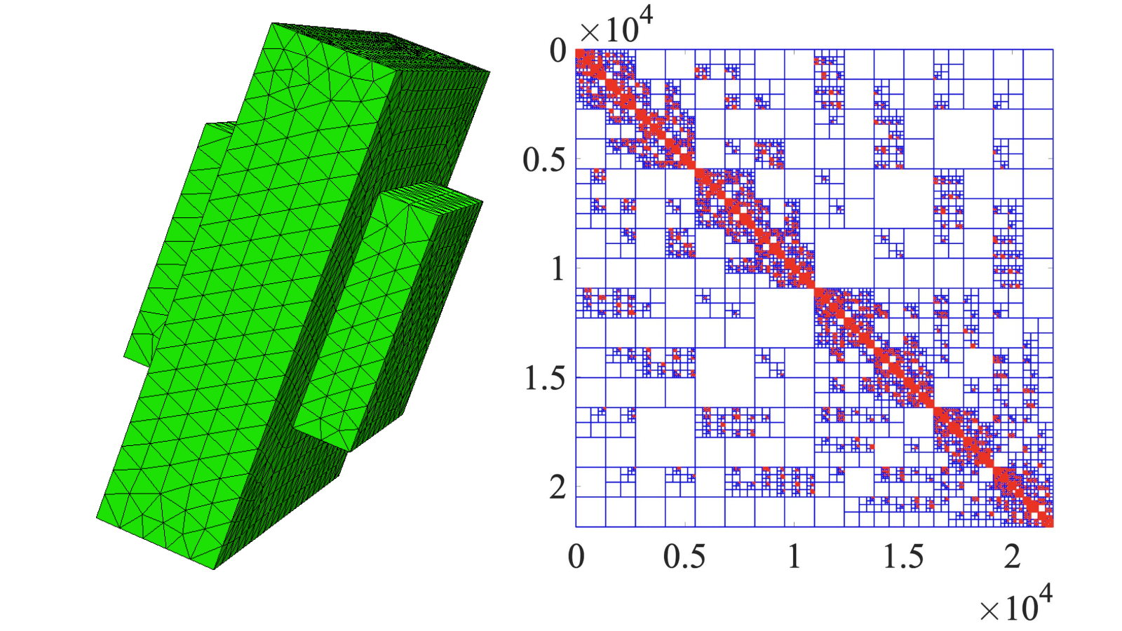
Here the geometry consists of two boxes, i.e., $\Omega:=(-1,1)\times(-1,1)\times[-1,-2)\cup(-2,2)\times[1,2)\times(-1,1)\cup(-2,2)\times[-1,1]\times[-1,1]\cup(-1,1)\times(-1,1)\times[1,2)\cup(-2,2)\times[-1,2)\times(-1,1)$ . We set the parameters $\kappa=1$ , $\boldsymbol{J}_{S}=[1,1,1]^{\top}$ , and $\beta=1$ . The computational domain with and the inverse of $\mathcal{H}$ -matrix approximation of the stiffness matrix is shown in Figure 1. We have 24 440 admissible blocks, 48 404 small blocks and the depth is 16. The decay of the approximation error versus $r$ and the corresponding allocated memory are shown in Figure 2. As shown, using higher $r$ gives rise to a reliable inverse of the $\mathcal{H}$ -matrix approximation. The computed $\textbf{B}_{\mathcal{H}}$ can be used as a preconditioner to solve the linear system (7) directly.

Refer to caption — Figure 1: Example 2. The computational geometry (left) and the inverse of $\mathcal{H}$ -matrix approximation of the stiffness matrix (7) $\mathcal{H}$ -matrix clustering (right) for $N_{\text{dof}}=22\,001$ .

4.3 Example 3: a magnet surrounded by air

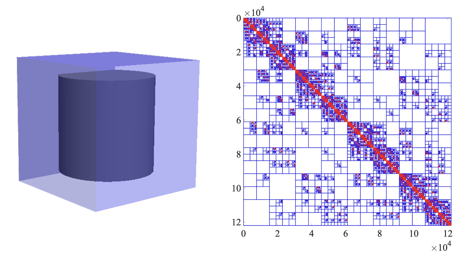
We consider a magnet surrounded by air where the box is $1\times 1\times 1$ and the magnet dimension is $0.5\times 0.5\times 0.75$ . We set $\kappa=10$ , $\beta=10$ and $\boldsymbol{J}_{S}=[10,10,10]^{\top}$ . The geometry and the $\mathcal{H}$ -approximation of A for $N_{\text{dof}}=122\,202$ is shown in Figure 3. In this approximation, we have 215 964 admissible blocks, 402 451 small blocks, and the depth is 15. The ${\mathcal{H}}-$ LU decomposition of A is given in Figure 4. We use Algorithm 1 for different $N_{\text{dof}}$ to solve the linear system. Table 2 shows the results for different matrices using $TOL=1\times 10^{-8}$ . For all cases, the negligible error indicates the accuracy the method, and the elapsed CPU time points out its efficiency. For the last two examples, we used Netgen/ngsolve schoberl2017netgen to produce the meshes (denoting different $N_{\text{dof}}$ ) and assembling the matrices of (7).

Table 2: The iterative solver preconditioned by

\mathcal{H}-LU

used to solve the Maxwell equations for different

N_{\text{dof}}

$N_{\text{dof}}$	5 492	8 050	13 602	33 933	48 811	70 133	78 603	96 846	129 200	304 309
error	7.22 e -9	1.07 e -9	5.80e-9	2.23e-8	5.11e-8	9.06e-8	5.98e-10	4.38e-10	5.04e-10	5.78e-9
time [s]	11.52	35.24	60.52	151.71	256.18	546.9	602.73	481	820.9	2335
iterations	3	3	3	3	4	4	5	5	6	7

5 Conclusion

In this work, the $\mathcal{H}$ -matrix approximation was used to solve the time-harmonic Maxwell equations. As a direct solver, the inverse of the hierarchical matrix approximation of the linear system was employed as a preconditioner, where an accurate approximation was achieved. Additionally, we then employed an $\mathcal{H}-LU$ factorization as a preconditioner.

In both cases, the use of $\mathcal{H}$ matrix approximations could reduce the computational cost and increase the accuracy of the solution. The $\mathcal{H}$ matrices can be coupled with the domain decomposition to take advantage of both approaches, i.e., to reduce the complexity and accelerate the convergence of the iterative solvers. This possibility will be addressed in the future papers.

Acknowledgements.

The authors acknowledge the Deutsche Forschungsgemeinschaft (DFG) under Germany Excellence Strategy within the Cluster of Excellence PhoenixD (EXC 2122, Project ID 390833453). Maryam Parvizi is funded by Alexander von Humboldt Foundation project named

\mathcal{H}

-matrix approximability of the inverses for FEM, BEM and FEM-BEM coupling of the electromagnetic problems. Finally, the authors thank Sebastian Kinnewig for fruitful discussions.

References

[1] M. Bebendorf. Hierarchical matrices. Springer, 2008.
[2] M. Bebendorf and F. Kramer. Hierarchical matrix preconditioning for low-frequency–full-maxwell simulations. Proceedings of the IEEE, 101(2):423–433, 2012.
[3] M. Bebendorf and J. Ostrowski. Parallel hierarchical matrix preconditioners for the curl-curl operator. Journal of Computational Mathematics, pages 624–641, 2009.
[4] O. G. Ernst and M. J. Gander. Why it is difficult to solve Helmholtz problems with classical iterative methods. pages 325–363. Springer, 2012.
[5] M. Faustmann, J. M. Melenk, and M. Parvizi. $\mathcal{H}$ -matrix approximability of inverses of FEM matrices for the time-harmonic Maxwell equations. Advances in Computational Mathematics, 48(5), 2022.
[6] L. Grasedyck, W. Hackbusch, and S. L. Borne. Adaptive geometrically balanced clustering of $\mathcal{H}$ -matrices. Computing, 73(1):1–23, 2004.
[7] W. Hackbusch. Hierarchical matrices: algorithms and analysis, volume 49. Springer, 2015.
[8] W. Hackbusch and B. N. Khoromskij. A sparse $\mathcal{H}-$ matrix arithmetic: general complexity estimates. Journal of Computational and Applied Mathematics, 125(1-2):479–501, 2000.
[9] S. Henneking and L. Demkowicz. A numerical study of the pollution error and dpg adaptivity for long waveguide simulations. Computers & Mathematics with Applications, 95:85–100, 2021.
[10] R. Hiptmair. Finite elements in computational electromagnetism. Acta Numerica, 11:237–339, 2002.
[11] J. W. Liu. The multifrontal method for sparse matrix solution: Theory and practice. SIAM Review, 34(1):82–109, 1992.
[12] J. M. Melenk and S. Sauter. Wavenumber explicit convergence analysis for galerkin discretizations of the helmholtz equation. SIAM Journal on Numerical Analysis, 49(3):1210–1243, 2011.
[13] P. Monk et al. Finite element methods for Maxwell’s equations. Oxford University Press, 2003.
[14] J. M. Ostrowski, M. Bebendorf, R. Hiptmair, and F. Krämer. $\mathcal{H}$ -matrix-based operator preconditioning for full maxwell at low frequencies. IEEE Transactions on Magnetics, 46(8):3193–3196, 2010.
[15] Y. Saad. Iterative methods for sparse linear systems. SIAM, 2003.
[16] J. Schöberl et al. Netgen/ngsolve. https://ngsolve.org, 2017.