Symmetry-breaking-induced loss of ergodicity in maps of the simplex with inversion symmetry

Systems of coupled maps were introduced as discrete time models for the dynamics of collective systems of interacting units [10]. They have revealed a rich phenomenology depending on the individual dynamics and on the coupling type and strength. Part of this phenomenology has been proved from a rigorous mathematical point of view [4].

In particular, the most common result in the chaotic (expanding or hyperbolic) setting is the existence of a unique absolutely continuous invariant measure (acim) when the coupling strength is sufficiently weak. Such uniqueness follows from perturbation arguments at the uncoupled limit, see e.g. [11] for piecewise expanding coupled maps with a finite number of units. For systems with infinitely many units, similar uniqueness statements have been proved in the case of nearest-neighbour or exponentially decaying coupling, see for instance [3, 9, 12, 16]. These results have been considered as the analogue in the deterministic setting of the theory of dynamical systems, of the uniqueness of the high temperature phase in particle systems of statistical mechanics, and especially in the Ising model.

The analogy with particle systems suggests that, when the coupling strength increases sufficiently, uniqueness of the acim (and hence ergodicity) should be lost via some analogue of a symmetry-breaking-induced phase transition [3]. Yet, the nature of this transition and its outcomes have long been debated in the community [4]. In particular, outside the weak coupling regime, the features of the symbolic dynamics on which the thermodynamics formalism and the subsequent theory of phase transitions are grounded, are not usually known with enough detail. In the setting of infinite lattices, exceptions have been provided by ad-hoc examples inspired by Toom’s cellular automata that exhibit standard phase transitions [1, 8].

Loss of ergodicity upon sufficient increase of the coupling strength also occurs in systems with finitely many units. This is particularly the case of the family $\{F_{N,\epsilon}\}_{\epsilon\in[0,\frac{1}{2})}$ of maps of the $N$-dimensional torus $\mathbb{T}^{N}$ defined by [13]¹¹ 1 We use $[1,N]$ to denote the collection of the first $N$ natural integers.

where²² 2 The symbol $\lfloor\cdot\rfloor$ denotes the floor function.

The maps $F_{N,\epsilon}$ are all expanding piecewise affine maps with expanding rate $2(1-\epsilon)\in(1,2]$ (see Appendix A for a summary of related notions). Their atoms are determined by the pairwise distances between the coordinates $\mathrm{u}_{i}$, whether they are smaller or larger than $\tfrac{1}{2}$. Moreover, the map $g$ commutes with the inversion symmetry $-\text{Id}|_{\mathbb{T}}$; likewise the maps $F_{N,\epsilon}$ commute with $-\text{Id}|_{\mathbb{T}^{N}}$. The $F_{N,\epsilon}$ also commute with every element of the group $\Pi_{N}$ of the permutations of the coordinates $\{\mathrm{u}_{i}\}_{i=1}^{N}$. Altogether, the $F_{N,\epsilon}$ can be considered as an elementary model of a system of $N$ chaotic units in interaction, where the discontinuities induced by $g$ play the role of nonlinearities.

For every $N$, the map $F_{N,\epsilon}$ can be shown to have an ergodic acim when $\epsilon$ is small enough (viz. expanding rate close to 2). Moreover, numerical simulations showed evidences of the breakdown of the inversion symmetry in the long-term dynamics, when $\epsilon$ is close enough to $\tfrac{1}{2}$ (ie. expanding rate close to 1) [5, 6]. The essential characteristics of this phenomenology is given in Appendix B, which in particular describes the systematic symmetric and asymmetric features of the various acim. This appendix also introduces an original representation of the trajectories that facilitates the visualization of these features.

The numerical evidences of loss of ergodicity have been partly confirmed by analytic and/or computer assisted proofs of the emergence of an asymmetric acim, namely an acim whose support is disjoint from its image under the coordinate sign inversion. That symmetry then implies the existence of a pair of acim with disjoint supports, which suffices to ensure that ergodicity in $F_{N,\epsilon}$ cannot hold. The analytic proofs applied to $N\in[3,4]$, see [5, 7, 17, 18], the computer-assisted ones to $N\in[3,6]$, see [6]. In both cases, they consisted in proving the existence of asymmetric invariant unions of polytopes (AsIUP), namely invariant unions of polytopes (IUP) that are disjoint from their image under the symmetry (see again Appendix A for the definitions).

While the proofs have been designed to be deployed in arbitrary dimension, the details of the dynamics of the AsIUP are specific to the value of $N$ under consideration. No simple mechanism has emerged that could be naturally extended to an arbitrary value of $N$ (NB: Specific limitations to such an extension are discussed at the beginning of Section 4 below). Accordingly, this paper more modestly aims to provide instances of families of maps in arbitrary dimension that capture some characteristics of the $F_{N,\epsilon}$ while exhibiting provable emergence of AsIUP via a simple systematic mechanism when their expanding rate is close to 1.

A natural source of inspiration for our study is to consider a simple example in one dimension, namely the family $\{f_{a}\}_{a\in(1,2)}$ of Lorenz-type maps with three branches, see Figure 1 and Appendix C. As the $F_{N,\epsilon}$, the maps $f_{a}$ are expanding piecewise affine and they commute with an inversion symmetry. Moreover, in agreement with the $F_{N,\epsilon}$ phenomenology described above (recall that the expanding rate of $F_{N,\epsilon}$ is equal to $2(1-\epsilon)$), $f_{a}$ is ergodic with unique acim when the expanding rate $a$ is close to 2, and has two acim with disjoint supports when $a$ is near 1.

Accordingly, we aim to provide some multi-dimensional analogues of the families of maps $\{f_{a}\}$ that capture some characteristics of the $F_{N,\epsilon}$. Focus will be made on the emergence of AsIUP. In particular, the multi-dimensional maps will be self-maps of the $(N-1)$-simplex $S_{N-1}$, where given an arbitrary $d\in\mathbb{N}$, $S_{d}$ is defined by

Indeed, a preliminary analysis in Section 2 concludes that AsIUP of the coupled map $F_{N,\epsilon}$ in $\mathbb{T}^{N}$ can be deduced from AsIUP of some related projected map in $S_{N-1}$, denoted $G_{N-1,\epsilon}$.³³ 3 Notice that similar $N-1$-dimensional reductions of the coupled map $F_{N,\epsilon}$ dynamics have already been identified [5, 18]. Yet these reductions yielded maps of $\mathbb{T}^{N-1}$ or of $[0,1]^{N-1}$, not of $S_{N-1}$. More precisely, an elementary reduction theory is developed in Section 2.1, for arbitrary maps of $\mathbb{T}^{N}$ that commute with every permutation of given $N-1$ coordinates. In the piecewise affine case, the theory shows that an IUP of the original map can be ensured by an IUP of some projected map of the subset $I_{N}\subset\mathbb{R}^{N}$ of points with increasing coordinates, see Lemma 2.2. Considerations about the transfer of an additional symmetry, typically an inversion symmetry, to a symmetry of the projected map are given in Section 2.2. For more specific mappings such as $F_{N,\epsilon}$, a further change of variables implies that it suffices to consider IUP of the map $G_{N-1,\epsilon}$, which also inherits some inversion symmetry from the $-\text{Id}|_{\mathbb{T}^{N}}$ of the $F_{N,\epsilon}$ (Section 2.3).

As a consequence, the desired multi-dimensional analogues of the map $f_{a}$ will be maps of $S_{N-1}$ that share some systematic features of the maps $G_{N-1,\epsilon}$. These features and the proposed mechanism for AsIUP are given in Section 3. In particular, Section 3.1 identifies the inversion symmetry, the outer atoms of the atomic collection and the dynamics in these atoms. This section also identifies the changes in the atomic collection as $N$ varies and hence, identifies some cause of the absence of full systematic in the features of the $G_{N-1,\epsilon}$.

Inspiration for a systematic mechanism for AsIUP in the arbitrary $d$-simplex is obtained in Section 3.2 from a thorough analysis of the dynamics of the family $\{G_{2,\epsilon}\}_{\epsilon\in(0,\frac{1}{2})}$, which turns out to show the same ergodic/non-ergodic features as the family $\{f_{a}\}$. As for the $f_{a}$, the mechanism consists in ensuring, for sufficiently small expanding rate, the existence of a simply-connected IUP lying across $A\cup B$ where $A$ is an outermost atom and the atom $B$ is adjacent to $A$ (see Claim 3.3 and Fig. 4). As for the $f_{a}$, the map restriction to $A$ (resp. to $B$) expands away from the corresponding fixed point so that the points are eventually mapped into $B$ (resp. into $A$). In $B$, this trend is combined with the action of a permutation in some basis attached to the fixed point. The latter feature is a purely multi-dimensional characteristic that has no analogue in dimension 1. In addition, the dynamics in the atoms $A$ and $B$ are such that the IUP does not intersect its symmetric image; hence providing an AsIUP.

With all the necessary elements being identified, the main result of the paper can finally be stated and proved (Theorem 4.1 in Section 4). This statement claims the existence, for an arbitrary integer $d\geq 3$, of a family of inversion-symmetric maps of the simplex $S_{d}$ that reproduce the common features of the maps $G_{d,\epsilon}$ and have AsIUP when the expanding rate is close enough to 1. The proof essentially consists in constructing the maps so that they exhibit some multi-dimensional extension of the symmetry-breaking mechanism in the family $\{G_{2,\epsilon}\}_{\epsilon\in(0,\frac{1}{2})}$. In particular, focus is made on constructing the analogue of the restriction to the atom $B$ above. The construction and associated mechanism are based on simple principles which should extend to a broad range of maps with permutation and inversion symmetries.

In order to define the projection procedure, we need to introduce various basic notions associated with the dynamics in $\mathbb{T}^{N}$ and its permutation symmetries. Given $N\in\mathbb{N}$, let

be the set of elements $\mathrm{u}\in\mathbb{T}^{N}$ whose coordinates are all distinct. The reason for considering $\mathbb{T}_{\ast}^{N}$ instead of $\mathbb{T}^{N}$ will be given below. Let then the map $P$ be defined by

This map is well-defined as a one-to-one mapping from $\mathbb{T}^{N}$ into $\mathbb{R}^{N}$. The set $D_{\ast}^{N}=P\mathbb{T}_{\ast}^{N}$ is a fundamental domain of $\mathbb{T}_{\ast}^{N}$ (namely, every element of $\mathbb{T}_{\ast}^{N}$ can be represented by a unique element in $D_{\ast}^{N}$), which reads

Let also $I_{N}\subset D_{\ast}^{N}$ be the subset of points with increasing coordinates, namely

For the sake of notations, we use the same symbol $\pi$ for a transformation that permutes the first $N-1$ coordinates in $\mathbb{T}^{N}$ and in $\mathbb{R}^{N}$ respectively (and likewise for $\Pi_{N-1}$). Given $u\in D_{\ast}^{N}$, let $\pi_{u}\in\Pi_{N-1}$ be such that $\pi_{u}u\in I_{N}$. The reason for dealing with $\mathbb{T}_{\ast}^{N}$ instead of $\mathbb{T}^{N}$ is that the ordering permutation $\pi_{u}$ is unique when $u\in D_{\ast}^{N}$. Notice also that, for every $u\in D_{\ast}^{N}$, the map $v\mapsto\pi_{u}v$ is invertible on $\mathbb{R}^{N}$. Moreover, we obviously have $\pi I_{N}\subset D_{\ast}^{N}$ for every $\pi\in\Pi_{N-1}$.

Assuming in addition that the map $F$ is non-singular, namely that the pre-images of zero Lebesgue measure sets have zero Lebesgue measure, so that $\mathrm{F}$ is also non-singular and then the complement set $I_{N}\setminus\left(I_{N}\cap\mathrm{F}^{-1}D_{\ast}^{N}\right)$ has zero Lebsegue measure. The relation (1) suggests to consider the projected map ${\cal F}$ defined in $I_{N}\cap\mathrm{F}^{-1}D_{\ast}^{N}$ by

The important features of ${\cal F}$ for our purpose, especially in the piecewise affine case, are identified in the following statement.

To see this, assume that $u\in\bigcup_{\pi\in\Pi_{N-1}}\pi A$. Then $u\in\pi A\subset D_{\ast}^{N}$ for some $\pi\in\Pi_{N-1}$. Also the symmetry of $F$ implies that $\pi A\subset\mathrm{F}^{-1}D_{\ast}^{N}$ for every $\pi\in\Pi_{N-1}$, which in particular yields $\pi_{u}u\in I_{N}\cap\mathrm{F}^{-1}D_{\ast}^{N}$. Relation (1) then implies

where $v=\pi_{\mathrm{F}\circ\pi_{u}u}\circ\mathrm{F}|_{I_{N}}\circ\pi_{u}u={\cal F}\circ\pi_{u}u\in A$ because $\pi_{u}u\in A$ and $A$ is invariant under ${\cal F}$. In other terms, $\mathrm{F}u\in\pi^{\prime}A$ for some $\pi^{\prime}\in\Pi_{N-1}$, proving invariance.

Moreover, that the union sets $\bigcup_{\pi\in\Pi_{N-1}}\pi A$ and $\bigcup_{\pi\in\Pi_{N-1}}\pi B$ are disjoint is also immediate. Firstly, when $\pi\neq\pi^{\prime}$, we must have $\pi A\cap\pi^{\prime}B=\emptyset$ because these sets belong to distinct regions of $D_{\ast}^{N}$ (distinct relative ordering of the coordinates). Secondly, if we had $\pi A\cap\pi B\neq\emptyset$ for some $\pi$, then we would have $A\cap B\neq\emptyset$ since $\pi$ is one-to-one, which contradicts the initial assumption.

In addition, the permutation symmetry group implies that for every $\omega^{\prime}$, we have $A^{\prime}_{\omega^{\prime}}=\pi A^{\prime}_{\omega^{\prime}_{+}}$ where $\pi\in\Pi_{N-1}$ and the index $\omega^{\prime}_{+}$ are such that $A^{\prime}_{\omega^{\prime}_{+}}\subset I_{N}$. Then, the map ${\cal F}$ is a piecewise affine map for the atomic collection $\{A^{\prime\prime}_{\omega^{\prime\prime}}\}$ defined by the refinement of $\{A^{\prime}_{\omega^{\prime}_{+}}\}$ by the sets in $I_{N}$ in which the ordering of the coordinates $((\mathrm{F}u)_{i})_{i=1}^{N-1}$ is constant (namely those sets in which the permutation $\pi_{\mathrm{F}u}$ does not depend on $u$).

Now, a similar reasoning as in the proof of (i) shows that if $\bigcup_{k}P_{k}$ and $\bigcup_{k^{\prime}}P^{\prime}_{k^{\prime}}$ are disjoint IUP for ${\cal F}$, then $\bigcup_{k}P_{k}$ and $\bigcup_{k^{\prime}}P^{\prime}_{k^{\prime}}$ must be disjoint IUP for $\mathrm{F}$. $\Box$

Following Lemma 2.2, a natural setting for the existence of multiple invariant sets/IUP for the projected map ${\cal F}$ is when this map has some symmetry, so that one can investigate the existence of asymmetric invariant sets/AsIUP. Accordingly, we need to determine those conditions that ensure that a (additional) symmetry of the original map $F$ transfers to one for ${\cal F}$. This is precisely the purpose of the following statement.

Since $F$ commutes with every $\pi\in\Pi_{N-1}$, it follows that, when $S$ satisfies the conditions of Lemma 2.3, every transformation $\pi\circ S$ induces a transformation $\pi\circ\Sigma$ with proper representation on $I_{N}$. Yet, that representation is identical to that of the original symmetry $S$, as our next claim states.

However when $F$ commutes with every permutation in $\Pi_{N}$, or more generally, when it commutes (only) with every element of the group $\Pi_{i_{1},\cdots,i_{N-1}}$ of the permutations of the $(N-1)$ coordinates indexed by $\{i_{1},\cdots,i_{N-1}\}$, a similar projection procedure as in the previous section can be defined, which is adapted to the $(N-1)$-uple under consideration. Naturally, the fundamental domain and corresponding projection $P$ depend on this $(N-1)$-uple, as well as do the representation of $F$ on the corresponding set $I_{N}$ of points with increasing coordinates and that of the inversion of sign coordinates $S$.

In short terms, when $F$ commutes with every permutation of all coordinates, both the projected map and the representation of the inversion of coordinate signs on $I_{N}$ are not unique and depend on the choice of the fundamental domain, see Appendix E for examples.

For the sake of notation, let $d=N-1$. As already pointed out, the coupled maps $F_{N,\epsilon}$ commute with every $\pi\in\Pi_{d}$, and also with the inversion symmetry $S=-\text{Id}|_{\mathbb{T}^{N}}$. The arguments above imply that when the corresponding projected map ${\cal F}_{N,\epsilon}$ defined by

(where $\mathrm{F}_{N,\epsilon}=P\circ F_{N,\epsilon}\circ P^{-1}$) has an AsIUP with respect to the inversion symmetry $\sigma_{\Sigma}$ defined by (3), then $F_{N,\epsilon}$ must have two acim with disjoint supports.

In addition, the specific form of the expression of $F_{N,\epsilon}$, namely that it consists of the sum of a multiple of the identity on $\mathbb{T}^{N}$ and a map that only depends on the coordinates differences $\mathrm{u}_{j}-\mathrm{u}_{i}$, implies a further reduction. To see this, let $\phi_{N}$ be defined by

This map is one-to-one and we have $\phi_{N}I_{N}=S_{d}\times[0,1)$, where $S_{d}$ is the $d$-simplex introduced in Section 1.2. Moreover, explicit computations yield the following statement.

Moreover, we have $\phi_{N}\circ\sigma_{\Sigma}\circ\phi_{N}^{-1}=\sigma_{d}\times\sigma^{\prime}_{1}$, where the inversion symmetries $\sigma_{d}$ and $\sigma^{\prime}_{1}$ respectively act on $S_{d}$ and $[0,1)$, and are given by

and

As a consequence, all the maps $G_{d,\epsilon}$ commute with $\sigma_{d}$.

Now, one can show that if $\bigcup_{k}P_{k}$ is an AsIUP of $G_{d,\epsilon}$ with respect to $\sigma_{d}$, then $\phi_{N}^{-1}\left(\bigcup_{k}P_{k}\times[0,1)\right)$ is an AsIUP of the projected map ${\cal F}_{N,\epsilon}$ with respect to $\sigma_{\Sigma}$. Accordingly, it suffices to obtain an AsIUP in $S_{d}$ of $G_{d,\epsilon}$ in order to show the existence of two acim with disjoint supports in $\mathbb{T}^{N}$ for the original coupled maps $F_{N,\epsilon}$.

A schematic summary of the whole reduction procedure associated with $F_{N,\epsilon}$ is given in Fig. 2.

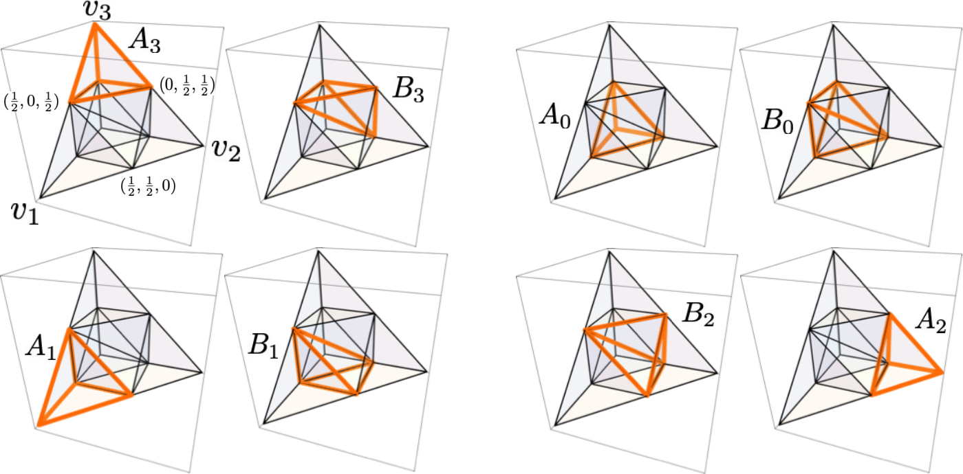
In order to state the features of $G_{d,\epsilon}$, we need to introduce and to describe the following subsets of $S_{d}$, see Fig. 3 and the left panel in Fig. 4.

• •

  Given $d\in\mathbb{N}$ and $k\in[0,d]$, let

  $$A_{0}=\left\{x\in S_{d}\ :\ x_{1}+\cdots+x_{d}<\tfrac{1}{2}\right\}\quad\text{and}\quad A_{k}=\left\{x\in S_{d}\ :\ \tfrac{1}{2}<x_{k}\right\},\ k\in[1,d].$$

• •

  For $d\geq 2$, let

  		$\displaystyle B_{0}=\left\{x\in S_{d}\ :\ x_{1}+\cdots+x_{d-1},x_{2}+\cdots+x_{d}<\tfrac{1}{2}<x_{1}+\cdots+x_{d}\right\}$
  		$\displaystyle B_{1}=\left\{x\in S_{d}\ :\ x_{1},x_{2}+\cdots+x_{d}<\tfrac{1}{2}<x_{1}+x_{2}\right\},$
  		$\displaystyle B_{k}=\left\{x\in S_{d}\ :\ x_{k}<\tfrac{1}{2}<x_{k-1}+x_{k},x_{k}+x_{k+1}\right\},\ k\in[2,d-1],$

  and

  $$B_{d}=\left\{x\in S_{d}\ :\ x_{1}+\cdots+x_{d-1},x_{d}<\tfrac{1}{2}<x_{d-1}+x_{d}\right\}.$$

Let $\{v_{k}\}_{k=0}^{d}$ be the collection of the vertices of $S_{d}$, where $v_{0}$ is the origin and where the coordinates of the other $v_{k}$ satisfy $(v_{k})_{i}=\delta_{i,k}$ for $i\in[1,d]$.

In addition, notice that the Lebesgue measure of the complement set $S_{d}\setminus\bigcup_{k}(A_{k}\cup B_{k})$ is zero for $d\in[2,3]$ and positive for $d\geq 4$.

Now, the next statement describes the main properties of the restrictions $G_{d,\epsilon}|_{A_{k}}$ and $G_{d,\epsilon}|_{B_{k}}$.

In order words, Lemma 3.2 states that $\{A_{k},B_{k}\}_{k=0}^{d}$ is an atomic collection of $G_{d,\epsilon}$ for $d\in[2,3]$, and also that $G_{d,\epsilon}$ has discontinuities inside every $B_{k}$ when $d\geq 4$. In the next section, we provide an analysis of the dynamics of $G_{2,\epsilon}$ and we establish the existence of AsIUP for $\epsilon$ near $\tfrac{1}{2}$.

As a preliminary comment to this section, we observe that for $d=1$, using that the interval $S_{1}=(0,1)=A_{0}\cup A_{1}\cup\{\tfrac{1}{2}\}$, the first claim in Lemma 3.2 entirely determines (up to a set of zero Lebesgue measure) the one-dimensional map $G_{1,\epsilon}:S_{1}\circlearrowleft$. This map is a particular case of a Lorenz map with two branches [15, 20] and has a unique ergodic acim for every value of $\varrho$ and $\epsilon$.

For $d=2$, we have $S_{2}=\overline{A_{0}\cup A_{1}\cup A_{2}\cup B}$ where $B:=B_{0}=B_{1}=B_{2}$ (see the left panel in Fig. 4). Lemma 3.2 states that the 2-dimensional map $G_{2,\epsilon}:S_{2}\circlearrowleft$ is an piecewise affine map with atoms $A_{0},A_{1},A_{2}$ and $B$. That statement also describes the action of the restrictions $G_{2,\epsilon}|_{A_{k}}$. As for the restriction $G_{2,\epsilon}|_{B}$, its expression is as follows (see equation (8) in Appendix D.1)

An analysis of this expression (details not shown) reveals that $G_{2,\epsilon}|_{B}$ has the following characteristics.

Let $C$ be the triangle with vertices $p_{0},p_{1}$ and $p_{2}$. The properties of $G_{2,\epsilon}$ on $A_{2}\cup B$ imply that the set $C\cup G_{2,\epsilon}C\subset\overline{A_{2}\cup B}$ is an IUP of $G_{2,\epsilon}$ when $\epsilon$ is close enough to $\tfrac{1}{2}$.⁷⁷ 7 Notice that $G_{2,\epsilon}|_{B}$ is not expanding but its second iterate $(G_{2,\epsilon}|_{B})^{2}$ is. This is sufficient to conclude that the IUP must contains an acim. The proof of this conclusion, which essentially consists in showing that $G_{2,\epsilon}(G_{2,\epsilon}C\cap A_{2})\subset G_{2,\epsilon}C$ when the expansion rate $2(1-\epsilon)$ is sufficiently close to 1, is sketched on Figure 4. The proof itself is an adaptation mutatis mutandis for $d=2$ of the proof of Proposition 4.5 below (details not shown).

References

- [1] J-B. Bardet and G. Keller, Phase transitions in a piecewise expanding coupled map lattice with linear nearest neighbour coupling, Nonlinearity 19 (2006), 2193-2210.
- [2] S. Boccaletti, J. Kurths, G. Osipov, D.L. Valladares and C.S. Zhou, The synchronization of chaotic systems, Phys. Rep. 366 (2002) 1-101.
- [3] L. Bunimovich and Y. Sinai, Space-time chaos in coupled map lattices, Nonlinearity 1 (1988) 491-516.
- [4] J-R. Chazottes and B. Fernandez (ed.), Dynamics of coupled map lattices and of related spatially extended systems, Lec. Notes Phys. Springer 671 (2005).
- [5] B. Fernandez, Breaking of ergodicity in expanding systems of globally coupled piecewise affine circle maps, J. Stat. Phys. 154 (2014) 999-1029.
- [6] B. Fernandez, Computer-assisted proof of loss of ergodicity by symmetry breaking in expanding coupled maps, Ann. H. Poincaré 21 (2020) 649-674.
- [7] B. Fernandez and F.M. Sélley, Conditioning problems for invariant sets of expanding piecewise affine mappings: Application to loss of ergodicity in globally coupled maps, Nonlinearity 35 (2022) 3991-4042.
- [8] G. Gielis and R. MacKay, Coupled map lattices with phase transitions, Nonlinearity 13 (2000), 867-888.
- [9] M. Jiang and Y. Pesin Equilibrium measures for coupled map lattices: existence, uniqueness and finite-dimensional approximations, Comm. Math. Phys. 193 (1998) 675-711.
- [10] K. Kaneko, Theory and applications of coupled map lattices, Wiley (1993).
- [11] G. Keller and M. Künzle, Transfer operators for coupled map lattices, Ergod. Th. Dynam. Sys. 12 (1992) 297-318.
- [12] G. Keller and C. Liverani, Uniqueness of the SRB measure for piecewise expanding weakly coupled map lattices in any dimension, Commun. Math. Phys. 262 (2006) 33 -50.
- [13] J. Koiller and L-S. Young, Coupled map networks, Nonlinearity, 23 (2010) 1121-1141.
- [14] G. Lancia and P. Serafini, Compact Extended Linear Programming Models, EURO Advanced Tutorials on Operational Research, Springer (2018).
- [15] W. Parry, The Lorenz attractor and a related population model in: M. Denker and K. Jacobs, (eds.) Ergodic Theory, Lect. Notes Math., 729 (1979) 169-187.
- [16] Y. Pesin and Y. Sinai, Space-time chaos in the system of weakly interacting hyperbolic systems, J. Geo. Phys. 3 (1988) 483-492.
- [17] F.M. Sélley, Symmetry breaking in a globally coupled map of four sites, Discrete & Cont. Dynam. Sys. A 38 (2018) 3707-3734.
- [18] F.M. Sélley and P. Bálint, Mean-field coupling of identical expanding circle maps, J. Stat. Phys., 164 (2016) 858-889.
- [19] M. Tsujii, Absolutely continuous invariant measures for expanding piecewise linear maps, Invent. Math. 143 (2001) 349–373.
- [20] R.F. Williams, The structure of Lorenz attractors, Pub. Math. IHES 50 (1979) 73-100.
Appendix A Essentials of expanding piecewise affine maps
Given , let be a bounded polytope or . A map is said to be a piecewise affine map of if there exists a finite collection of open, convex and disjoint polytopes included in (and called atoms) such that
- •
the difference set has zero Lebesgue measure,
for each , the restriction is an affine map and .
Notice that the atomic collection is not unique. One may choose any finite sub-collection of atoms such that