Report: Statistics of approximations to zeroes of $\zeta$-function via truncated symmetrized Euler products

Gonek, Hughes and Keating developed a hybrid formula [2] which aprroximates $\zeta(s)$ in terms of $P_{X}(s)$, a weighted version of the truncated Euler Product and $Z_{X}(s)$, a expression involving zeta-zeroes close to $s$:

where $P_{X}(s):=\exp(\sum_{n\leq X}\frac{\Lambda(n)}{n^{s}\log n})$.
Using this they conjectured the values of the moments of Zeta Function, by calculating moments of $P_{X}$ and $Z_{X}$ separately and multiplying them together. These conjectures match the known values of the first few moments.

Instead of truncating the Dirichlet series and symmetrizing it, we can try to do the same for the Euler product. However, symmetrizing with $1-s$ leads to bad approximations. Instead, Gonek [1] showed symmetrizing with $\overline{s}$ gives much better results. We define the approximations as:

Note that on the critical line, $\overline{s}=1-s$. Also, $\zeta_{X}(s)$ is not an analytic function, instead it is a harmonic function. Assuming RH, it approximates $\zeta(s)$ well to the right of the critical line.

It can be easily shown that $\zeta_{X}(s)$ satisfies the Riemann Hypothesis:

Looking at plots of $\zeta_{X}(s)$ and $\zeta(s)$ on the critical line, we see that even for low values of X, the zeroes of $\zeta_{X}$ are quite close to zeta zeroes (figure as provided in [1]):

From [1, pg.  2170] we have that on the critical line, $|\chi(1/2+it)|=1$ for $|t|\geq C_{0}$. Also, $|P_{X}(s)|=|P_{X}(\overline{s})|$. Hence, $\zeta_{X}(s)=P_{X}(s)\left(1+\chi(s)\frac{P_{X}(s)}{P_{X}(s)}\right)$ vanishes for $|t|\geq C_{0}$ if and only if $\arg\left(\chi(s)P_{X}(s)/P_{X}(\overline{s})\right)\equiv\pi(\text{mod }2\pi)$.

As with Gonek’s paper, we work with a slight modification of $F_{X}$ to simplify our expressions. We define:

We then have $F_{X}^{\star}(t)=F_{X}(t)+O(\frac{X}{\tau^{2}\log X})$, hence for values of $X\leq t^{2}$, these are close. For $F_{X}^{\star}(t)$ we have the simpler expression:

We compare the graphs of $N(t)$ and $1+\frac{1}{2\pi}F_{X}^{\star}(t)$:

As we see in the figure 3, the actual zeroes and approximate zeroes are quite close to each other. Also, around a zeta zero the slope stays relatively constant. For the zeta-zero $\gamma_{0}$, let the approximate zero be $\tilde{\gamma_{0}}$, and their difference is $\delta=\gamma_{0}-\tilde{\gamma_{0}}$.

Let $H_{X}^{\star}:=\frac{1}{2\pi}F_{X}^{\star}+1$. At $\tilde{\gamma_{0}}$, $H_{X}^{\star}$ takes the value $N(T)-\frac{1}{2}$. Then, by simple geometry we have

Looking at 4, at $t=\gamma_{0}$,

Hence, we have:

$F_{2}$ decreases for bigger values, according to $F_{2}(z)\ll\frac{\exp(\max(-\Re\,z,-\Re\,2z))}{|z|^{2}}$. Hence we look at the contribution of zeroes close to $\gamma_{0}$.

We observe some of the statistics of zeroes when X is fixed, say X=5:

We can see that most of the differences are very small but in general the differences tend to increase as we look at higher zeroes.

Looking at the two neighbouring zeroes, we define:

where $\gamma_{n}$ is the $n^{\text{th}}$ zeta-zero ordinate.

Similarly we can look at more neighbouring zeroes. However this approach is possibly fruitless as we consider higher ordinates, justified in Section 4.1.

As we mentioned before, to approximate the expression around $t=\gamma_{0}$, we choose $X=\frac{\gamma_{0}}{2\pi}$.

We can see that most of the differences are very small but unlike the differences tend to increase as we look at higher zeroes.

Let us first look at some numerical evidence.

As one can see, the slopes are near constant in the neighbourhood of the zeta-zero ordinates.

We calculate the slopes and plot them:

The slopes closely resemble a logarithmic graph. We can deduce a formula for it later. For now, we work with the numerical values. So, according to our heuristic , scaling the differences by our slopes should give us the right hand side of equation 7. We do so here ¹¹ 1 I had to weed out some anomalies (about 10 whose values were way off). There were probably because of errors in calculating our near-constant slope due to shortcomings in our code. I will later try to rescale the differences again with the theoretical value for the slope.:

From Gonek’s paper [1, pg./,2175], we have,

Changing the x-axis of our graph from the ‘$N^{\text{th}}$ zero’ to ‘Ordinate t’, we use Mathematica to get the best fit log curve as $-0.6+3.1\log(\frac{t}{2\pi})$. The R-Squared value is 99.327 %. I’ve plotted the data with the fitted curve below:

Similar to 8, looking at the two neighbouring zeroes, we define:

where $\gamma_{n}$ is the $n^{\text{th}}$ zeta-zero ordinate.

Plotting it for the first 2000 zeroes, we get:

If we squint a bit, this resembles the shape of the distribution we get in our actual scaled differences in Figure 8. More notably, the majority of the values are recorded between -0.2 and 0.2 in both the figures.

The main difference between the model and the actual histogram is that the model lacks a lot of values which lie in the region 0.05 to 0.15 (and symmetrically on the other side too). It can be heuristically explained by the fact that, in the infinite sum, we can pair up zeroes on the left of $\gamma_{0}$ to the right of it. Most of the time they cancel out as they have similar absolute values. The values in this region 0.05 to 0.15 arises when these pairings don’t cancel each other out, which is more likely once we consider more and more pairings instead of just 1 pair.

As a follow-up to our last observation we look at the statistics for two pairs of adjacent zeroes. Defining an analogous model as 9, we consider two pairs of adjacent zeroes. We place the results one after the other for comparison ²² 2 I’ve cleaned up some of the more extreme values ($\geq 0.3$) in 8 so that the histograms match up in their width:

As we had remarked before, due to more scope of uneven cancellation between pairs of zeroes, there is more “meat” around the central spike in Figure 21.

What we want to study in this section is, what is the probability that the first/second model gives answers close to the actual scaled difference. The motivation for this lies in remark 4.1 in the next section.

At a given zeta-zero ordinate $\gamma_{n}$,we have the actual scaled difference $D_{n}$ and the value given by the model $M_{n}$. The relative error in the model be $E_{n}=\frac{|D_{n}-M_{n}|}{D_{n}}$. Given a sample of values of n from $N$ to $600$, we want to calculate for what percentage of the sample $E_{n}<\frac{1}{5}$. We do this for the first and second model:

Ideally we are looking for large values of ordinates. We see that for the first model, we have small error for $6\%$ of the time, whereas for the second model it is around $10\%$.

Looking at $X=\lfloor\gamma_{0}/{2\pi}\rfloor\sim\tau/{2\pi}$, the second term in Equation 10 can be bounded as:

If we take $\Delta=C\frac{2\pi}{\log\tau}$. We take constant C such that for large ordinates this term has a smaller order than the first term .

Now, looking at the first term we have:

We calculate the variances for $X=3$ to $27$ and $X=30,35,\dots,65$ and $X=100$. Here’s what they look like for some of them:

As we can see the plots resemble some sort of logarithmic growth as the ordinate increases. Also notice that as X increases the variances also decrease. This is expected.

We calculate the absolute errors as X varies like $X=\frac{t}{2\pi}$ and then scale them by inverse of mean density as before. We do this for up to first 5000 zeroes and zeroes 10,000 to 11,000. We take the moving variance (200 points) of these values to make it more smooth. The results are:

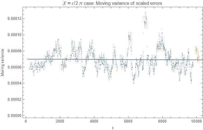
In the previous report we had hoped that these errors would remain bounded uniformly even for high ordinates and that looking at a few adjacent zeroes would give a good idea of the distribution of errors. Figure 17 confirms this.

If we look at the histogram of scaled errors at various points of the sample, we see the following trend:

The distribution remains similar for higher ordinates.

We recall what we observed in the first report where we took more and more adjacent zeroes in our models³³ 3 Another reminder that here we are scaling by the slope and not by the density, but it only amounts to a factor of $\frac{3}{2\pi}$:

Hence our initial guess that using a few pairs of adjacent zeroes can model the error distribution consistently is true. Otherwise the distribution would’ve become “fatter” for higher ordinates to incorporate more uneven cancellations from more terms.

We try to find a model for the moving variances we had in Figure 16. Let’s say the moving variances behave like $A(X)B(t)$. The method I have used is:

1. 1.

   Guess a model for $B(t)$ such as $\log^{k}(t)$, $t^{k}$, $W(t)^{k}$ (Lambert W function) or $t^{k_{1}}\log^{k_{2}}(t)$.
   For example, take $B(t)=\log^{k}(t)$ here:
   

   

2. 2.

   With the ability to manipulate k, take $X=20$. Remember, we have the moving variance for this upto $10^{5}$ zeroes. First restrict to the sample of $5000$ zeroes and find the best fit coefficient $a_{1}$ to our chosen model of $B(t)$. Now take the full sample of $10^{5}$ zeroes and find the best fit coefficient $a_{2}$.

3. 3.

   Vary k to find the point where the difference $|a_{1}-a_{2}|$ is the lowest. This is the value of $k$ we will consider henceforth.

   In the example of $\log^{k}(t)$ considered in Figure 22, $k=4.3$ seems to have the lowest difference in coefficients.

4. 4.

   Now, vary X and at each step find the best fit coefficient for our model $B(t)$ (with the value of k found in step 3). These will be the values for A(X).

5. 5.

   Plot the values of $A(X)$ for the different X and find the best fit model in a similar way to $B(t)$.

   In our example of $B(t)=\log^{4.3}(t)$, we find the coefficients A(X) have the following values:

   

   Here, $A(X)=\frac{5.02365\times 10^{-6}}{\log^{3.13788}(X)}$ is the best fit curve derived from sample X = 11 to 26, but also seem to model the values from X = 30 to 100 very well.

   Hence our model predicts that $V_{\text{model}}(x,t)=\frac{5.02365\times 10^{-6}}{\log^{3.13788}(x)}\log^{4.3}(t)$. If we try plugging in $x=\frac{t}{2\pi}$, we get $V_{\text{model}}(t)\sim 5.02365\times 10^{-6}{\log^{1.16}(t)}$. This certainly means the errors for $\zeta_{\frac{t}{2\pi}}$ increase logarithmically for higher ordinates. However this model isn’t quite right as it misses our plot by some margin:

   

   We should try some other models for $B(t)$ and compare.

$B(t)$ is modelled as $W(t)^{3.7}$. An ideal $k$ turns out to be something around 3.7. Finding a suitable $A(x)=\frac{2.528\times 10^{-5}}{W^{3.6}(x)}$, our model becomes:

We see that the model is somewhat close to the actual values of the variance recorded.

References

- [1] S. Gonek, Finite euler products and the riemann hypothesis, Transactions of the American Mathematical Society, 364 (2012), pp. 2157–2191.
- [2] S. M. Gonek, C. P. Hughes, and J. P. Keating, A hybrid Euler-Hadamard product for the Riemann zeta function, Duke Mathematical Journal, 136 (2007), pp. 507 – 549.
- [3] E. C. Titchmarsh and D. R. Heath-Brown, The theory of the Riemann zeta-function, Oxford science publications, Clarendon Press ; Oxford University Press, Oxford : New York, 2nd ed , revised by d.r. heath-brown ed., 1986.