Scalable Collaborative Learning via Representation Sharing
Abstract
Privacy-preserving machine learning has become a key conundrum for multi-party artificial intelligence. Federated learning (FL) and Split Learning (SL) are two frameworks that enable collaborative learning while keeping the data private (on device). In FL, each data holder trains a model locally and releases it to a central server for aggregation. In SL, the clients must release individual cut-layer activations (smashed data) to the server and wait for its response (during both inference and back propagation). While relevant in several settings, both of these schemes have a high communication cost, rely on server-level computation algorithms and do not allow for tunable levels of collaboration. In this work, we present a novel approach for privacy-preserving machine learning, where the clients collaborate via online knowledge distillation using a contrastive loss (contrastive w.r.t. the labels). The goal is to ensure that the participants learn similar features on similar classes without sharing their input data. To do so, each client releases averaged last hidden layer activations of similar labels to a central server that only acts as a relay (i.e., is not involved in the training or aggregation of the models). Then, the clients download these last layer activations (feature representations) of the ensemble of users and distill their knowledge in their personal model using a contrastive objective. For cross-device applications (i.e., small local datasets and limited computational capacity), this approach increases the utility of the models compared to independent learning and other federated knowledge distillation (FD) schemes, is communication efficient and is scalable with the number of clients. We prove theoretically that our framework is well-posed, and we benchmark its performance against standard FD and FL on various datasets using different model architectures.
1 Introduction
Motivated by concerns such as data privacy, large scale training and others, Machine Learning (ML) research has seen a rise in different types of collaborative ML techniques. Collaborative ML is typically characterized by an orchestrator algorithm that enables training ML model(s) over data from multiple owners without requiring them to share their sensitive data with untrusted parties. Some of the well known algorithms include Federated Learning (FL) [36], Split Learning (SL) [16] and Swarm Learning [54]. While the majority of the works in collaborative ML rely upon a centralized coordinator, in this work, we design a decentralized learning framework where the server plays a secondary role and could easily be replaced by a peer-to-peer network. As we show in the rest of the paper, the main benefit of our decentralized approach over centrally coordinated ML is the increased flexibility among clients in controlling the information flow across different aspects such as communication, privacy, computational capacity, data heterogeneity, etc.
Most existing collaborative learning schemes are built upon FL, where the training algorithm and/or the model architecture is usually imposed to the clients to match the computational capacity of the weaker participant (or the server). We refer to this property as non-tunable collaboration, since the degree of collaboration is mostly imposed by the server. While this is less of a problem in cross-silo applications (small number of data owners, large local datasets) since the participants can easily find consensus over the best training parameters, it can constitute a strong barrier for participation in cross-device applications (large number of users with small local datasets and low/heterogeneous computational capacity). Indeed, finding consensus becomes harder in that scenario. To alleviate this, we propose a new framework for tunable collaboration, i.e., where each participant has near total control over its data release, its model architecture and how the knowledge of other users should be integrated in its own personalized model.
Our main idea is to share learned feature representations of each class among users and to use these representations cleverly during local training. Since the clients can choose which features are aggregated and shared, our framework enables the clients to assign different privacy levels to different samples. Our decentralized approach also ensures that the overall system remains asynchronous and functions as expected even if all but two clients are offline in the whole system. Finally, our framework makes it convenient to account for model heterogeneity and model personalization, since every user can select a subset of peers based on their goals of generalization and personalization. While some of these advantages have been introduced in recent FL based schemes, our framework allows natural integration of such several ideas. Our work is different from the body of work done in FL due to its decentralized design. Specifically, our system does not use server-level computation algorithms that are directly involved in the training of the model. Nevertheless, for completeness, we experimentally compare it with FL in Section 3.
Our contribution can be summarized as follows:
- •
We present a new tunable collaborative learning algorithm based on contrastive representation learning and online knowledge distillation.
- •
We prove theoretically that our local objective is well-posed.
- •
We show empirically the advantages of our framework against other similar schemes in terms of utility, communication, and scalability.
2 Related Work
Federated Learning
FL is considered to be the first formal framework for collaborative learning. In their initial paper, McMahan et al. 2017 introduce a new algorithm called FedAvg, in which each client performs several optimization steps on their local private dataset before sending the updated model back to the server for aggregation using weight averaging. While this approach alleviates the communication cost of the baseline collaborative optimization algorithm FedSGD, it also decreases the personalization capacity of the global model due to the naive model averaging, especially in heterogeneous environments. Several algorithms have been proposed to address these limitations, in particular FedProx [30], FedPer [4], FedMa [52], FedDist [43], FedNova [53], Scaffold [23] and VRL-SGD [32].
Concerning the server update, Reddi et al. 2020 introduce federated versions of existing adaptive optimization algorithms like Adagrad, Adam and Yogi, and Michieli and Ozay 2021 present FedProto, where an attention mechanism is used for clever aggregations. The attention coefficients are computed using prototypes (i.e., per class averages of last hidden layer activations, a.k.a. feature representations). While our framework also uses such prototypes, it is conceptually very different as we use them directly in the local objective function (and not in the aggregation).
Although all these algorithms usually improve the convergence rate, they suffer from the same constraints as FedAvg, i.e., homogeneous model architecture for every client, high communication overhead and non-tunable collaboration, all potential barriers for participation.
Fully Decentralized Learning
The use of a central server in traditional FL constitutes a single point of failure and can also become a bottleneck when the number of clients grows, as shown by Lian et al. 2017. To alleviate these issues, Vanhaesebrouck et al. 2016 formalize a new framework where each client participates in the learning task via a peer-to-peer network using gossip algorithms [44, 13]. In this configuration, there is no global solution and each client has its own personalized model, which enables both personalization and generalization. On the other hand, it creates other challenges about convergence, practical implementation and privacy [22]. Moreover, as in FL, the entire model must be released at every communication round, which can constitute a barrier for participation for the same reasons.
Knowledge Distillation


The concept of knowledge distillation (KD) originated in Bucila et al. 2006 as a way of compressing models, and was later generalized by Hinton et al. 2015 (see Gou et al. 2021 for an overview of the field). The standard use case for KD is that of a Teacher-Student (or offline) configuration, in which the teacher model (usually a large and well-trained model) transfers its knowledge to the student model (usually a smaller model) by sharing its last layer activations on a given transfer dataset (see Fig. 1(a)). The knowledge is then distilled into the student model using a divergence loss between the teacher and student models outputs (response-based KD) or intermediate layers (feature-based KD) on the transfer dataset. Traditional KD schemes use a transfer set that is similar (or identical) to the teacher training dataset, but some recent work has focused on data-free (or zero-shot) KD. This can be achieved either by looking at some of the teacher model statistics to generate synthetic transfer data [35, 39, 6], or by training a GAN in parallel [37, 10, 2]. It has also been shown that positive results can be obtained using mismatched or random unlabeled data for the distillation [27, 40]. A key concept for our framework is the idea of online KD (or co-distillation [3], see Fig. 1(b)), where each model is treated as both a teacher and a student, meaning that the KD is performed synchronously with the training of each model (rather than after the training of the teacher model) [15, 57, 45]. Finally, ensemble KD (see Fig. 1(c)) refers to the setup where the knowledge is distilled from an ensemble of teacher (offline) or teacher-student (online) models.
Collaborative Learning via Knowledge Distillation
A growing body of literature has recently investigated ways of using online knowledge distillation (KD) [8, 19] for collaborative learning in order to alleviate the need of sharing model updates (FL) or individual smashed data (SL). He et al. 2020 introduce FedGKT, where clients and servers exchange activations in order to consolidate the training. Similarly, Jeong et al. 2018 present Federated Knowledge Distillation (FD), where each client uploads its mean (per class) logits to a central server, who aggregates and broadcasts them back. These soft labels are then used as the teacher output for the KD loss during local training. A closely related idea is to compute the mean logits on a common public dataset [29, 20, 9], but we argue that selecting this dataset can induce bias and is not always feasible, since additional trust is needed for its selection, and sufficient relevant data might be lacking. Besides FD, KD can enable collaborative learning in various ways: In an attempt to decrease the communication cost, Wu et al. 2022 introduce FedKD, in which each client trains a (large) teacher network on their private data and transfer locally its knowledge to a smaller student model, which is then used in a standard FL algorithm. On the other hand, Lin et al. 2020 and Chen and Chao 2020 use KD on an unlabeled synthetic or public dataset to make the FL aggregation algorithm more robust. Our approach differs significantly from these schemes, as it does not rely on traditional FL algorithms.
3 Methods

Preamble and Motivation
Consider any classification task on -dimensional raw inputs with distinct classes and a set of participating users , each with a local private dataset and a model :
where represents the joint probability of choosing a user and drawing a sample from its distribution, and , represent the linear classifier and neural network (up to last hidden layer) of user , respectively (with potentially different architectures across users). More precisely, let be the output dimension of and be model weights of user . We have:
where and are the raw input, the feature representation and the logits, respectively. We motivate our approach as follows. Assuming no sharing of raw data (for privacy concerns), any collaborative learning framework falls in one of two buckets: weight sharing or activation sharing. As mentioned in Section 2, sharing weights (i.g., FL) comes with strong constraints (communication, model architecture, etc.) and might not always be suitable. Concerning activation sharing (i.g., SL), it can be done at any layer (hidden or output). However, since activations are usually strongly correlated to the raw input [51], sharing single sample activations can raise privacy concerns. Instead, sharing averaged activations can easily be met with differential privacy guarantees (see privacy in Section 3). Due to the high non-linearity of neural networks, sharing averaged activations only makes sense at the output layer or last hidden layer (since the classifier is linear). Sharing only averaged outputs (averaged over samples of the same class) like in FD has been shown to have limited success as the quantity of shared information is restricted to the dimension of the output , and we argue in this paper that sharing the feature representations (i.e., outputs of the last hidden layer, also averaged over samples of the same class) is more flexible and leads to better results. In this light, our objective is to collaboratively learn the best feature representation for each class, using contrastive (w.r.t. classes) representation learning [46] and feature-based knowledge distillation [14]. In other words, we want to learn collaboratively (i.e., only once) the structure of the feature representation space so that each client does not need to find it on its own with its limited amount of data and/or computational capacity.
Contrastive Objective
In this section, we introduce a contrastive objective function for private online knowledge distillation (i.e., when users synchronously learn personalized models without sharing their raw input data and by collaborating via online distillation). This new objective function and its derivation are partly inspired by the offline contrastive loss presented in Tian et al. 2020 and van den Oord et al. 2018, with a few important differences. In the offline non-private setting, both the teacher and student models and have access to the same dataset . In that scenario, the representations and are pulled apart if and are pulled together if . However, in the private setting, does not have access to the raw input data that was used to train the teacher model, but has its own private dataset. At a given communication round and from the perspective of user , we define as the student model and as the teacher model, where is a user selected at random. Consider the following procedure: samples from its own data distribution and then samples either jointly (i.e., from the same observation of ) or independently (from two independent observations of ) the two random vectors and defined as follows:
| (1) | ||||||
| (2) |
The parameter defines over how many samples we take the average, which in turn defines the concentration of the distribution of . From the (student) perspective of client and in the spirit of collaboration, the goal is to maximize the mutual information . Still from the perspective of , let , and be the joint and marginal distributions of and , respectively, and let be a Bernoulli random variable indicating if a tuple has been drawn from the joint distribution or from the product of marginals . Finally, let be the joint distribution of such that and and suppose that the prior satisfy and , i.e., for each sample from the distribution , we draw samples from the distribution . We can show the following bound.
Theorem 1.
Using the above notation, let be any estimate of with Bernoulli parameter , and let be defined as follows:
| (3) |
The mutual information can be bounded as
| (4) |
with equality iff (better estimates lead to tighter bounds). The proof is joined in the supplementary material.
Hence, by minimizing in Eq. (4), we optimize a lower bound on the mutual information . Taking advantage of the classifier , a natural choice for is the discriminator with Bernoulli parameter
| (5) |
With this choice, can be interpreted as the estimated probability that the features and come from the same class. Note that in their work, Tian et al. 2020 train an external discriminator (i.e., that is not defined using the model classifier ).
Final Objective
Intuitively, from the perspective of , minimizing ensures that its classifier can distinguish if two feature representations, one local and one from another user, come from the same class. To improve the algorithm convergence and to ensure that can classify the feature representation of another client (similar as in Invariant Risk Minimization [5]), we also introduce a classical feature-based KD term . This term minimizes the distance between the local and global feature representations of a same class (we define the global representation of class as the expected value ). An important distinction between and is that the first one uses an inter-client averaged representation, whereas the second one uses an intra-client averaged representation. Combining and with the standard cross-entropy loss using the meta parameters and , the final optimization problem of becomes:
| (6) |
Implementation
With the standard assumption that the datasets are composed of IID samples drawn from their corresponding distributions, the expected losses and can be approximated by their unbiased mini-batch estimators and , respectively. For one given sample, the loss functions are given by , and finally
| (7) |
Finally, for the sampling procedure of the contrastive objective, we use the most intuitive scheme: for every training sample with feature representation , we use one observation of sampled using (i.e., ), and one observation of sampled using each (i.e., ). Thus, we have . With these considerations, a detailed description of our collaborative learning framework can be found in the supplementary material.
Communication
In terms of communication, the uplink and downlink volumes are of order and per round, where and represent the number of realizations (per class) that are uploaded and downloaded by the clients, respectively (these parameters can be tuned to match the communication capacity of the network). For comparison, these volumes are of order and for FL (with the model size) and and for SL. Because in most scenarios and since and are tunable, we observe that our framework is communication efficient compared to FL and SL.
Relaxation to peer-to-peer
We emphasize here that our contrastive objective is fully compatible with a peer-to-peer configuration, since the server only acts as a relay for the observations of . For the traditional feature-based KD objective , we use one global representation per class (i.e., one for the whole network), which in theory can only be computed by a central entity. One way to alleviate this could be to use the average of all the observations of that were downloaded by user as a proxy for the global feature representations. However, to focus solely on the effectiveness of the proposed objectives rather than the topology of the network, we only present experiments in which a central entity computes the global representations.
Privacy
Our framework naturally attains a certain degree of privacy by sharing representations from the penultimate layer, which, as per information bottleneck principle [47], has minimal mutual information from the original data. Although such a level of privacy may not be enough from a membership attack point of view, we emphasize that the privacy is amplified by averaging out these representations, hence amplifying the privacy of individual samples. To further make our framework formally private, we propose using recent progress in differentially private mean estimation [34, 7] to obtain a differentially private mean before it gets shared with other clients. Furthermore, our framework naturally dovetails with recent works [25, 1] in variable privacy levels for different samples. The users can assign variable levels of privacy to different samples before they get aggregated in a privacy preserving manner.
4 Experiments
Datasets, models and training
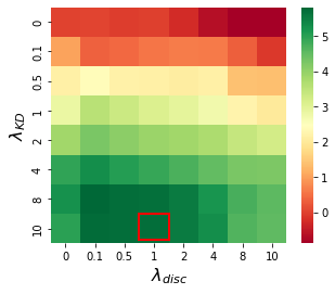
We run several experiments with the MNIST [12], Fashion-MNIST [56] and CIFAR10 [26] datasets. For MNIST, we use a simple convolutional neural network (CNN) similar to LeNet5 ( parameters) [28] and for Fashion-MNIST and CIFAR10, we use ResNet9 ( parameters) and ResNet18 ( parameters) architectures [18], respectively. For the dimension of feature representation space, we set for LeNet5, for ResNet9 and for ResNet18. In order to simulate a scenario where the data is sparse, we only select a fraction of the train dataset (1200 samples for MNIST, 6000 for Fashion-MNIST and 10000 for CIFAR10) that we split uniformly at random across users. For the validation, we use the entire test dataset for each task (10000 samples). In order to have fair comparisons, we train all the models for the same number of communication rounds, and we stop the training as soon as framework has reasonably converged ( for MNIST/LeNet5, for Fashion-MNIST/ResNet9 and CIFAR10/ResNet18). We compare our framework with centralized learning (or CL, i.e., with and ), independent learning (or IL, i.e., with ), federated learning using FedAvg (FL) and federated knowledge distillation (FD). We use the default learning rate for all experiments and we perform 1 local epoch of training per communication round. For CL, IL, FD and our framework, we use the Adam stochastic optimization algorithm [24]. Finally, supported by Fig. 3, we set and in our final objective (Eq. (6)).
Network emulation
For our contrastive objective , we use (i.e., for every class, each user selects samples of that class, computes and averages their feature representations, uploads them to the server and downloads the representations of another user chosen at random). For the feature-based KD objective , each client average the feature representation of all the samples of a same class and uploads these averaged representations to the server, which in turn averages them to obtain one global representation per class. For simplicity, we use (clients upload and download one observation of for each class).
Software and hardware
We use the CUDA enabled PyTorch library [41] with a GTX 1080 Ti (11GB) GPU and an Intel(R) Xeon(R) CPU (2.10GHz).
5 Discussion
Utility
As seen in Table 1, our framework outperforms every other framework for when a small model is used (MNIST/LeNet5), especially when the number of clients grows, which is typically the kind of configuration that would be relevant for a cross-device application). In that setup, FL performs particularly poorly as it struggles to find a low-capacity model that matches the data distribution of each client. This is particularly visible on Fig. 4(b). Although in that configuration, FD shows similar performance for small number of clients (), it still exhibits a lower rate of convergence (compare Fig. 4(c) and Fig. 4(d)). Our framework even outperforms centralized learning (CL) when , suggesting that the added objectives can also be seen as regularizers. For the Fashion-MNIST dataset, our framework shows significant improvement over IL and FD (i.e., frameworks where there are no global model), but is not able to compete with FL anymore, which in that case even outperforms CL. However, the comparison between FL and our framework is unfair for large models due to the amounts of shared information (i.g., for ResNet9, one communication round of our framework communicates times fewer bits than standard FL. This ratio increases to for ResNet19). Similar conclusions can be drawn for the CIFAR10 experiments. However, in that case, even IL outperforms our framework for after rounds. Indeed, since our objective function is highly complex (the global minimum depends on the data of other peers), the algorithm struggles to converge to the optimal model when the number of parameters is very large. However, we argue that this is not critical since training ResNet18 models on low capacity devices is not particularly adapted to cross-device applications, as they usually require powerful GPUs and large datasets to converge.


| MNIST () | Fashion-MNIST () | CIFAR10 () | |||||||
| CL | 94.00 | 87.77 | 66.15 | ||||||
|
|
|
|
|
|
|
|
|
| |
| FL | 92.64 | 86.79 | 70.06 | 89.79 | 89.28 | 88.21 | 67.99 | 59.18 | 51.05 |
| IL | 91.46 | 85.26 | 72.86 | 86.04 | 83.61 | 80.52 | 59.85 | 46.46 | 38.51 |
| FD | 94.45 | 90.55 | 77.90 | 87.17 | 83.32 | 79.44 | 56.75 | 44.91 | 31.43 |
| Ours | 94.19 | 90.63 | 82.07 | 87.91 | 84.44 | 80.77 | 63.49 | 47.28 | 37.78 |
Effect of
The feature-based KD term makes sure that similar feature representations are learned by each client. Fig. 5 provides insight into the evolution of the latent feature space during training. In FL, the structure of the latent feature space is imposed from the start to each client, whereas in our framework, clients have more freedom to learn the best structure that fits their data, since they are only guided towards a global representation structure. This clearly improves convergence, as we can see that clusters are already formed at round 25 with our algorithm, whereas with FL the latent feature space is still relatively chaotic at that point. On the other hand, we observe that for IL, the learned latent feature space is totally different for each client as they learn it by themselves, and the convergence rate is also notably slower (compare round 25 for instance).

Effect of
The effect of the contrastive objective is more subtle, but can still improve the test accuracy significantly if tuned properly. In fact, whereas can be used without , the reciprocal is not true as observed on Fig. 3. This is because we have defined the discriminator of user (i.e., ) using its feature representation classifier (see Eq. (5)). Hence, in order to generate useful gradients for back propagation (i.e., that do not look like noise), must be able to classify relatively well the feature representations that are generated by other models. We have also tested external discriminators (like in [46]), but the results were not as positive.
Limitations and Future work
As shown by the results, our approach is particularly relevant when the model capacity is relatively small, but struggles when the model complexity grows, especially when compared with FL. However, the comparison is unfair in that scenario, as the amount of information that is shared between clients at each round is larger by several orders of magnitudes for FL. We also posit that the convergence gap could be reduced by adding sophistication into the algorithm (i.g., by having a local algorithm that selects the most relevant observed representations from other users, by only sharing a fraction of the feature representation dimensions, by introducing a more complex discriminator , etc.). Another important limitation is the fact that our framework cannot be used for supervised tasks other than classification, as the feature representations need to be sorted by class. This is harder to alleviate since the whole system’s architecture is build upon this requirement. Future work should also investigate how the number of class and their distributions might influence the performance of the algorithm, and also if (and how) it could be used for unsupervised learning.
6 Conclusion
We introduce a new collaborative learning algorithm that enables tunable collaboration in cross-device applications and whose uplink and downlink communication does not scale with the model size (as in FL) or the dataset size (as in SL). We prove that our objective is well posed from the point of view of collaboration, as it maximizes a lower bound on the mutual information between the feature representations of different users across the network. Then, we show empirically that it is particularly relevant in setups where the number of clients is large and when each of them have limited computational resources. In that scenario, it converges faster than IL, FD and even standard FL. Due to its simplicity and modularity with other potential requirements (such as differential privacy, server free/peer-to-peer configurations, heterogeneous model architectures, etc.), we posit that our algorithm could be implemented in numerous settings where FL (or other similar frameworks) is not suitable, as long as careful task-specific deployment considerations are made.
Acknowledgments and Disclosure of Funding
Living and travel expenses of the main author partially supported by the Hasler Foundation and EPFL.
References
- Acharya et al. [2020] Jayadev Acharya, Kallista Bonawitz, Peter Kairouz, Daniel Ramage, and Ziteng Sun. Context aware local differential privacy. In International Conference on Machine Learning, pages 52–62. PMLR, 2020.
- Addepalli et al. [2020] Sravanti Addepalli, Gaurav Kumar Nayak, Anirban Chakraborty, and Venkatesh Babu Radhakrishnan. Degan: Data-enriching gan for retrieving representative samples from a trained classifier. In Proceedings of the AAAI Conference on Artificial Intelligence, volume 34, pages 3130–3137, 2020.
- Anil et al. [2018] Rohan Anil, Gabriel Pereyra, Alexandre Passos, Róbert Ormándi, George E. Dahl, and Geoffrey E. Hinton. Large scale distributed neural network training through online distillation. CoRR, abs/1804.03235, 2018. URL http://arxiv.org/abs/1804.03235.
- Arivazhagan et al. [2019] Manoj Ghuhan Arivazhagan, Vinay Aggarwal, Aaditya Kumar Singh, and Sunav Choudhary. Federated learning with personalization layers. CoRR, abs/1912.00818, 2019. URL http://arxiv.org/abs/1912.00818.
- Arjovsky et al. [2019] Martin Arjovsky, Léon Bottou, Ishaan Gulrajani, and David Lopez-Paz. Invariant risk minimization, 2019.
- Bhardwaj et al. [2019] Kartikeya Bhardwaj, Naveen Suda, and Radu Marculescu. Dream distillation: A data-independent model compression framework, 2019. URL https://arxiv.org/abs/1905.07072.
- Brown et al. [2021] Gavin Brown, Marco Gaboardi, Adam Smith, Jonathan Ullman, and Lydia Zakynthinou. Covariance-aware private mean estimation without private covariance estimation. Advances in Neural Information Processing Systems, 34, 2021.
- Bucila et al. [2006] Cristian Bucila, Rich Caruana, and Alexandru Niculescu-Mizil. Model compression. In Proceedings of the 12th ACM SIGKDD International Conference on Knowledge Discovery and Data Mining, KDD ’06, page 535–541, New York, NY, USA, 2006. Association for Computing Machinery. ISBN 1595933395. doi: 10.1145/1150402.1150464. URL https://doi.org/10.1145/1150402.1150464.
- Chang et al. [2019] Hongyan Chang, Virat Shejwalkar, Reza Shokri, and Amir Houmansadr. Cronus: Robust and heterogeneous collaborative learning with black-box knowledge transfer, 2019. URL https://arxiv.org/abs/1912.11279.
- Chen et al. [2019] Hanting Chen, Yunhe Wang, Chang Xu, Zhaohui Yang, Chuanjian Liu, Boxin Shi, Chunjing Xu, Chao Xu, and Qi Tian. Data-free learning of student networks. In Proceedings of the IEEE/CVF International Conference on Computer Vision, pages 3514–3522, 2019.
- Chen and Chao [2020] Hong-You Chen and Wei-Lun Chao. Feddistill: Making bayesian model ensemble applicable to federated learning. CoRR, abs/2009.01974, 2020. URL https://arxiv.org/abs/2009.01974.
- Deng [2012] Li Deng. The mnist database of handwritten digit images for machine learning research. IEEE Signal Processing Magazine, 29(6):141–142, 2012.
- Dimakis et al. [2010] Alexandros G. Dimakis, Soummya Kar, José M. F. Moura, Michael G. Rabbat, and Anna Scaglione. Gossip algorithms for distributed signal processing. Proceedings of the IEEE, 98(11):1847–1864, 2010. doi: 10.1109/JPROC.2010.2052531.
- Gou et al. [2021] Jianping Gou, Baosheng Yu, Stephen J Maybank, and Dacheng Tao. Knowledge distillation: A survey. International Journal of Computer Vision, 129(6):1789–1819, 2021.
- Guo et al. [2020] Qiushan Guo, Xinjiang Wang, Yichao Wu, Zhipeng Yu, Ding Liang, Xiaolin Hu, and Ping Luo. Online knowledge distillation via collaborative learning. In Proceedings of the IEEE/CVF Conference on Computer Vision and Pattern Recognition (CVPR), June 2020.
- Gupta and Raskar [2018] Otkrist Gupta and Ramesh Raskar. Distributed learning of deep neural network over multiple agents. Journal of Network and Computer Applications, 116:1–8, 2018.
- He et al. [2020] Chaoyang He, Murali Annavaram, and Salman Avestimehr. Group knowledge transfer: Federated learning of large cnns at the edge. In H. Larochelle, M. Ranzato, R. Hadsell, M.F. Balcan, and H. Lin, editors, Advances in Neural Information Processing Systems, volume 33, pages 14068–14080. Curran Associates, Inc., 2020. URL https://proceedings.neurips.cc/paper/2020/file/a1d4c20b182ad7137ab3606f0e3fc8a4-Paper.pdf.
- He et al. [2016] Kaiming He, Xiangyu Zhang, Shaoqing Ren, and Jian Sun. Deep residual learning for image recognition. In Proceedings of the IEEE conference on computer vision and pattern recognition, pages 770–778, 2016.
- Hinton et al. [2015] Geoffrey Hinton, Oriol Vinyals, Jeff Dean, et al. Distilling the knowledge in a neural network. arXiv preprint arXiv:1503.02531, 2(7), 2015.
- Itahara et al. [2020] Sohei Itahara, Takayuki Nishio, Yusuke Koda, Masahiro Morikura, and Koji Yamamoto. Distillation-based semi-supervised federated learning for communication-efficient collaborative training with non-iid private data. CoRR, abs/2008.06180, 2020. URL https://arxiv.org/abs/2008.06180.
- Jeong et al. [2018] Eunjeong Jeong, Seungeun Oh, Hyesung Kim, Jihong Park, Mehdi Bennis, and Seong-Lyun Kim. Communication-efficient on-device machine learning: Federated distillation and augmentation under non-iid private data. CoRR, abs/1811.11479, 2018. URL http://arxiv.org/abs/1811.11479.
- Kairouz et al. [2021] Peter Kairouz, H Brendan McMahan, Brendan Avent, Aurélien Bellet, Mehdi Bennis, Arjun Nitin Bhagoji, Kallista Bonawitz, Zachary Charles, Graham Cormode, Rachel Cummings, et al. Advances and open problems in federated learning. Foundations and Trends® in Machine Learning, 14(1–2):1–210, 2021.
- Karimireddy et al. [2020] Sai Praneeth Karimireddy, Satyen Kale, Mehryar Mohri, Sashank Reddi, Sebastian Stich, and Ananda Theertha Suresh. Scaffold: Stochastic controlled averaging for federated learning. In International Conference on Machine Learning, pages 5132–5143. PMLR, 2020.
- Kingma and Ba [2014] Diederik P Kingma and Jimmy Ba. Adam: A method for stochastic optimization. arXiv preprint arXiv:1412.6980, 2014.
- Kotsogiannis et al. [2020] Ios Kotsogiannis, Stelios Doudalis, Sam Haney, Ashwin Machanavajjhala, and Sharad Mehrotra. One-sided differential privacy. In 2020 IEEE 36th International Conference on Data Engineering (ICDE), pages 493–504. IEEE, 2020.
- [26] Alex Krizhevsky, Vinod Nair, and Geoffrey Hinton. Cifar-10 (canadian institute for advanced research). URL http://www.cs.toronto.edu/˜kriz/cifar.html.
- Kulkarni et al. [2017] Mandar Kulkarni, Kalpesh Patil, and Shirish Subhash Karande. Knowledge distillation using unlabeled mismatched images. CoRR, abs/1703.07131, 2017. URL http://arxiv.org/abs/1703.07131.
- LeCun et al. [1989] Y. LeCun, B. Boser, J. S. Denker, D. Henderson, R. E. Howard, W. Hubbard, and L. D. Jackel. Backpropagation Applied to Handwritten Zip Code Recognition. Neural Computation, 1(4):541–551, 12 1989. ISSN 0899-7667. doi: 10.1162/neco.1989.1.4.541. URL https://doi.org/10.1162/neco.1989.1.4.541.
- Li and Wang [2019] Daliang Li and Junpu Wang. Fedmd: Heterogenous federated learning via model distillation. CoRR, abs/1910.03581, 2019. URL http://arxiv.org/abs/1910.03581.
- Li et al. [2020] Tian Li, Anit Kumar Sahu, Manzil Zaheer, Maziar Sanjabi, Ameet Talwalkar, and Virginia Smith. Federated optimization in heterogeneous networks. Proceedings of Machine Learning and Systems, 2:429–450, 2020.
- Lian et al. [2017] Xiangru Lian, Ce Zhang, Huan Zhang, Cho-Jui Hsieh, Wei Zhang, and Ji Liu. Can decentralized algorithms outperform centralized algorithms? a case study for decentralized parallel stochastic gradient descent. Advances in Neural Information Processing Systems, 30, 2017.
- Liang et al. [2019] Xianfeng Liang, Shuheng Shen, Jingchang Liu, Zhen Pan, Enhong Chen, and Yifei Cheng. Variance reduced local SGD with lower communication complexity. CoRR, abs/1912.12844, 2019. URL http://arxiv.org/abs/1912.12844.
- Lin et al. [2020] Tao Lin, Lingjing Kong, Sebastian U Stich, and Martin Jaggi. Ensemble distillation for robust model fusion in federated learning. Advances in Neural Information Processing Systems, 33:2351–2363, 2020.
- Liu et al. [2021] Xiyang Liu, Weihao Kong, Sham Kakade, and Sewoong Oh. Robust and differentially private mean estimation. Advances in Neural Information Processing Systems, 34, 2021.
- Lopes et al. [2017] Raphael Gontijo Lopes, Stefano Fenu, and Thad Starner. Data-free knowledge distillation for deep neural networks. CoRR, abs/1710.07535, 2017. URL http://arxiv.org/abs/1710.07535.
- McMahan et al. [2017] Brendan McMahan, Eider Moore, Daniel Ramage, Seth Hampson, and Blaise Aguera y Arcas. Communication-efficient learning of deep networks from decentralized data. In Artificial intelligence and statistics, pages 1273–1282. PMLR, 2017.
- Micaelli and Storkey [2019] Paul Micaelli and Amos J Storkey. Zero-shot knowledge transfer via adversarial belief matching. Advances in Neural Information Processing Systems, 32, 2019.
- Michieli and Ozay [2021] Umberto Michieli and Mete Ozay. Prototype guided federated learning of visual feature representations. CoRR, abs/2105.08982, 2021. URL https://arxiv.org/abs/2105.08982.
- Nayak et al. [2019] Gaurav Kumar Nayak, Konda Reddy Mopuri, Vaisakh Shaj, Venkatesh Babu Radhakrishnan, and Anirban Chakraborty. Zero-shot knowledge distillation in deep networks. In International Conference on Machine Learning, pages 4743–4751. PMLR, 2019.
- Nayak et al. [2021] Gaurav Kumar Nayak, Konda Reddy Mopuri, and Anirban Chakraborty. Effectiveness of arbitrary transfer sets for data-free knowledge distillation. In Proceedings of the IEEE/CVF Winter Conference on Applications of Computer Vision (WACV), pages 1430–1438, January 2021.
- Paszke et al. [2019] Adam Paszke, Sam Gross, Francisco Massa, Adam Lerer, James Bradbury, Gregory Chanan, Trevor Killeen, Zeming Lin, Natalia Gimelshein, Luca Antiga, Alban Desmaison, Andreas Kopf, Edward Yang, Zachary DeVito, Martin Raison, Alykhan Tejani, Sasank Chilamkurthy, Benoit Steiner, Lu Fang, Junjie Bai, and Soumith Chintala. Pytorch: An imperative style, high-performance deep learning library. In Advances in Neural Information Processing Systems 32, pages 8024–8035. Curran Associates, Inc., 2019. URL http://papers.neurips.cc/paper/9015-pytorch-an-imperative-style-high-performance-deep-learning-library.pdf.
- Reddi et al. [2020] Sashank J. Reddi, Zachary Charles, Manzil Zaheer, Zachary Garrett, Keith Rush, Jakub Konečný, Sanjiv Kumar, and H. Brendan McMahan. Adaptive federated optimization. CoRR, abs/2003.00295, 2020. URL https://arxiv.org/abs/2003.00295.
- Sannara et al. [2021] EK Sannara, François Portet, Philippe Lalanda, and VEGA German. A federated learning aggregation algorithm for pervasive computing: Evaluation and comparison. In 2021 IEEE International Conference on Pervasive Computing and Communications (PerCom), pages 1–10. IEEE, 2021.
- Shah [2009] Devavrat Shah. Gossip algorithms. Found. Trends Netw., 3(1):1–125, jan 2009. ISSN 1554-057X. doi: 10.1561/1300000014. URL https://doi.org/10.1561/1300000014.
- Sodhani et al. [2020] Shagun Sodhani, Olivier Delalleau, Mahmoud Assran, Koustuv Sinha, Nicolas Ballas, and Michael G. Rabbat. A closer look at codistillation for distributed training. CoRR, abs/2010.02838, 2020. URL https://arxiv.org/abs/2010.02838.
- Tian et al. [2020] Yonglong Tian, Dilip Krishnan, and Phillip Isola. Contrastive representation distillation. In International Conference on Learning Representations, 2020. URL https://openreview.net/forum?id=SkgpBJrtvS.
- Tishby and Zaslavsky [2015] Naftali Tishby and Noga Zaslavsky. Deep learning and the information bottleneck principle. In 2015 ieee information theory workshop (itw), pages 1–5. IEEE, 2015.
- van den Oord et al. [2018] Aäron van den Oord, Yazhe Li, and Oriol Vinyals. Representation learning with contrastive predictive coding. CoRR, abs/1807.03748, 2018. URL http://arxiv.org/abs/1807.03748.
- van der Maaten and Hinton [2008] Laurens van der Maaten and Geoffrey Hinton. Visualizing data using t-sne. Journal of Machine Learning Research, 9(86):2579–2605, 2008. URL http://jmlr.org/papers/v9/vandermaaten08a.html.
- Vanhaesebrouck et al. [2016] Paul Vanhaesebrouck, Aurélien Bellet, and Marc Tommasi. Decentralized collaborative learning of personalized models over networks. CoRR, abs/1610.05202, 2016. URL http://arxiv.org/abs/1610.05202.
- Vepakomma et al. [2020] Praneeth Vepakomma, Abhishek Singh, Otkrist Gupta, and Ramesh Raskar. Nopeek: Information leakage reduction to share activations in distributed deep learning. In 2020 International Conference on Data Mining Workshops (ICDMW), pages 933–942. IEEE, 2020.
- Wang et al. [2020a] Hongyi Wang, Mikhail Yurochkin, Yuekai Sun, Dimitris S. Papailiopoulos, and Yasaman Khazaeni. Federated learning with matched averaging. CoRR, abs/2002.06440, 2020a. URL https://arxiv.org/abs/2002.06440.
- Wang et al. [2020b] Jianyu Wang, Qinghua Liu, Hao Liang, Gauri Joshi, and H Vincent Poor. Tackling the objective inconsistency problem in heterogeneous federated optimization. Advances in neural information processing systems, 33:7611–7623, 2020b.
- Warnat-Herresthal et al. [2021] Stefanie Warnat-Herresthal, Hartmut Schultze, Krishnaprasad Lingadahalli Shastry, Sathyanarayanan Manamohan, Saikat Mukherjee, Vishesh Garg, Ravi Sarveswara, Kristian Händler, Peter Pickkers, N Ahmad Aziz, et al. Swarm learning for decentralized and confidential clinical machine learning. Nature, 594(7862):265–270, 2021.
- Wu et al. [2022] Chuhan Wu, Fangzhao Wu, Lingjuan Lyu, Yongfeng Huang, and Xing Xie. Communication-efficient federated learning via knowledge distillation". Nat Commun, 13(1):2032, apr 2022.
- Xiao et al. [2017] Han Xiao, Kashif Rasul, and Roland Vollgraf. Fashion-mnist: a novel image dataset for benchmarking machine learning algorithms. CoRR, abs/1708.07747, 2017. URL http://arxiv.org/abs/1708.07747.
- Zhang et al. [2018] Ying Zhang, Tao Xiang, Timothy M Hospedales, and Huchuan Lu. Deep mutual learning. In Proceedings of the IEEE conference on computer vision and pattern recognition, pages 4320–4328, 2018.
Checklist
The checklist follows the references. Please read the checklist guidelines carefully for information on how to answer these questions. For each question, change the default [TODO] to [Yes] , [No] , or [N/A] . You are strongly encouraged to include a justification to your answer, either by referencing the appropriate section of your paper or providing a brief inline description. For example:
- •
Did you include the license to the code and datasets? [Yes] See Section .
- •
Did you include the license to the code and datasets? [No] The code and the data are proprietary.
- •
Did you include the license to the code and datasets? [N/A]
Please do not modify the questions and only use the provided macros for your answers. Note that the Checklist section does not count towards the page limit. In your paper, please delete this instructions block and only keep the Checklist section heading above along with the questions/answers below.
- 1.
For all authors…
- (a)
Do the main claims made in the abstract and introduction accurately reflect the paper’s contributions and scope? [Yes]
- (b)
Did you describe the limitations of your work? [Yes] See Section 5.
- (c)
Did you discuss any potential negative societal impacts of your work? [N/A]
- (d)
Have you read the ethics review guidelines and ensured that your paper conforms to them? [Yes]
- (a)
- 2.
If you are including theoretical results…
- (a)
Did you state the full set of assumptions of all theoretical results? [Yes]
- (b)
Did you include complete proofs of all theoretical results? [Yes] See Appendix A.2.
- (a)
- 3.
If you ran experiments…
- (a)
Did you include the code, data, and instructions needed to reproduce the main experimental results (either in the supplemental material or as a URL)? [Yes]
- (b)
Did you specify all the training details (e.g., data splits, hyperparameters, how they were chosen)? [Yes] See Section 3.
- (c)
Did you report error bars (e.g., with respect to the random seed after running experiments multiple times)? [Yes] Shaded area represents the std over clients (Fig. 4)
- (d)
Did you include the total amount of compute and the type of resources used (e.g., type of GPUs, internal cluster, or cloud provider)? [Yes] See Section 3.
- (a)
- 4.
If you are using existing assets (e.g., code, data, models) or curating/releasing new assets…
- (a)
If your work uses existing assets, did you cite the creators? [Yes] (MNIST, Fashion-MNIST and CIFAR10 datasets).
- (b)
Did you mention the license of the assets? [Yes]
- (c)
Did you include any new assets either in the supplemental material or as a URL? [Yes]
- (d)
Did you discuss whether and how consent was obtained from people whose data you’re using/curating? [N/A] We only use public datasets.
- (e)
Did you discuss whether the data you are using/curating contains personally identifiable information or offensive content? [N/A] We only use public datasets.
- (a)
- 5.
If you used crowdsourcing or conducted research with human subjects…
- (a)
Did you include the full text of instructions given to participants and screenshots, if applicable? [N/A]
- (b)
Did you describe any potential participant risks, with links to Institutional Review Board (IRB) approvals, if applicable? [N/A]
- (c)
Did you include the estimated hourly wage paid to participants and the total amount spent on participant compensation? [N/A]
- (a)
Appendix A Appendix
A.1 Notation
- •
: Number of participating users/clients/peers/data owners.
- •
: Raw input data dimension (e.g., for RBG images).
- •
: Latent feature (or feature representation) space dimensionality (i.e., width of last hidden layer).
- •
: Number of class.
- •
: Labeled data sample.
- •
: Joint probability density function across users.
- •
: Data distribution of user .
- •
: Dataset of user .
- •
with : Parameters of the neural network of , with the achievable model parameters for user .
- •
: Neural network of (or similar parameterized function) that maps a raw input into a latent feature space.
- •
: Linear classifier of .
- •
: Hyperparameters.
- •
: Learning rate.
- •
: Cross-entropy, feature-based KD and discriminator loss functions, respectively.
- •
: Expected value (over the data) of and , respectively.
- •
: Mini-batch estimates of and , respectively.
- •
: Random vectors (feature representations) of the student (user ) and the teacher (random user ).
- •
: Joint and marginal distributions of and , respectively.
- •
: Joint distribution of and , where is a binary random variable indicating if has been drawn from () or ().
- •
: Binary discriminator with Bernoulli parameter (i.e., learnable estimate of ).
- •
: Observation/realization of and , respectively.
- •
: Global (i.e., using all the samples across users) and local (i.e., using samples) average feature representations of class , respectively.
A.2 Proof of Theorem 1
Recall that is the joint distribution of such that and and suppose that the prior satisfy and , i.e., for each sample from the distribution , we draw samples from the distribution . We have:
| (8) | ||||
| (9) | ||||
| (10) | ||||
| (11) |
where the last equality is obtained using the Bayes’ rule on the posterior :
| (12) | ||||
| (13) | ||||
| (14) |
Hence, by optimizing with respect to the model parameters of the student, we optimize a lower bound on the mutual information between . By noting that , we can further bound the expectation term in (11) as follows:
| (15) | ||||
| (16) | ||||
| (17) | ||||
| (18) |
However, similar to Tian et al. 2020, the Bernoulli distribution is unknown and must therefore be approximated by training a discriminator . Using Gibbs’ inequality, we obtain
| (19) |
where the right-hand term is the expected negative log-likelihood loss of the discriminator for a particular set . Hence, Eq. (18) is proportional to minus the expected loss of the discriminator. Let denote the Bernoulli parameter of given the data (i.e., ), we define our learning objective for the discriminator as follows:
| (20) | ||||
| (21) | ||||
| (22) | ||||
| (23) | ||||
| (24) |
which concludes the derivation.