Phase transition and higher order analysis of $L_{q}$ regularization under dependence

The goal of linear regression is to estimate the parameter vector $\mbox{\boldmath$\beta$}_{0}\in\mathbb{R}^{p}$ from a set of $n$ response variables ${\bf y}\in\mathbb{R}^{n}$ under the model

where ${\bf X}\in\mathbb{R}^{n\times p}$ is a known measurement matrix and ${\bf w}\in\mathbb{R}^{n}$ is a noise vector. We consider the popular class of $L_{q}$-regularized least square methods (LQLS), given by the optimization problem

where $\|\cdot\|_{q}$ $(0\leq q\leq 2)$ denotes the $L_{q}$-norm and $\lambda\geq 0$ is a fixed number.

In many modern statistical applications with large $p$, the true $\mbox{\boldmath$\beta$}_{0}$ vector is often sparse, i.e. only $k$ of the elements of $\mbox{\boldmath$\beta$}_{0}$ are non-zero and the rest are zero. We would like to identify the useful predictors and also obtain good estimates of their coefficients. Among all LQLSs, the case $q=1$, or in other words $L_{1}$ optimization a.k.a. LASSO, is the most popular and best studied scheme for identifying a set of relevant features from a given list. LASSO enjoys attractive statistical properties (Fu and Knight 2000; Donoho 2006; Meinshausen and Bühlmann 2006) and has been effectively used for simultaneously producing accurate and parsimonious models.

However, as a convex relaxation of $L_{0}$-norm, the $L_{1}$-norm may be sub-optimal for recovering a real sparse signal because it tends to result in biased estimation by shrinking all the entries toward to zero simultaneously, and sometimes leads to over-penalization. Many researchers have shown that using the $L_{q}$-norm $(0\textless q\textless 1)$ to approximate the $L_{0}$-norm is in fact a better choice than using the $L_{1}$-norm because the former provides a tighter optimization relaxation to the original $L_{0}$ sparsity finding formulation. For example, in the noiseless settings ($w=0$), Chartrand and Staneva 2008; Saab et al. 2008; Saab and Özgür Yılmaz 2010 have shown that the global minima of (2) for $q\textless 1$ outperforms the solution of LASSO. They have derived the Restricted Isometry Property conditions that can guarantee the accurate recovers of the sparse vector from (2).

To understand the behavior of these algorithms in high dimension more reliably, a new asymptotic has been proposed recently which assumes that $p,n,k\rightarrow\infty$ with fixed $k/p=\epsilon$ and $n/p=\delta$. One of the main studies undertaken in this asymptotic framework is to find the relationship between the sparsity of the vector $\mbox{\boldmath$\beta$}_{0}$ and the successful recovery of it using $L_{q}$-minimization algorithm (2) under the noiseless setting. In other word, for different values of $\delta$, we need to know the boundary of sparsity $\epsilon$ that differentiates the success and failure of recovering by $L_{q}$-minimization. This boundary is known as the phase transition curve.

Stojnic 2013 characterizes the phase transition curve for the case of $q=0$. Wang et al. 2011 analyzes the phase transition curve for $\delta\rightarrow 1$. Kabashima et al. 2009 and Rangan et al. 2009 derives the exact value of phase transition curve for any value of $0\leq q\leq 1$ and any value of $\delta$ using the non-rigorous replica method. In addition to the sharp characterization of the phase transition in noiseless case, Weng et al. 2016; Zheng et al. 2017 also present accurate calculation of the mean squared error (MSE) in the presence of noise and compare the accuracy of estimator (2) for different values of $q$ under the optimal tuning of the parameter $\lambda$. They observe that if the measurement noise $w$ is zero or small, then the global minima of (2) for $q\textless 1$ (when $\lambda$ is optimally picked) outperforms the solution of LASSO with optimal $\lambda$. Furthermore, all values of $q\textless 1$ have the same performance when $w=0$. When $w$ is small, LQLS with the value of $q$ closer to 0 has a better performance. This coincides with the intuition that the performance of $L_{q}$- minimization is improved when $q$ decreases since it is closer to $L_{0}$-minimization. The analysis of Zheng et al. 2017 is based on approximate message passing (AMP) algorithm and replica method.

The phase transition of LQLS in the case $1\textless q\leq 2$, also known as bridge regression, has been thoroughly studied in last several decades with different techniques, such as combinatorial geometry (Donoho and Tanner 2005), statistical dimension framework (Amelunxen et al. 2013), Gordon’s lemma (Thrampoulidis et al. 2018), and AMP (Donoho et al. 2011; Weng et al. 2018; Wang et al. 2020; Ma et al. 2019). It was summarized in Weng et al. 2018; Weng and Maleki 2019; Wang et al. 2021 that the phase transition curve is $\delta_{q}(\epsilon)=1$ if $2\geq q\textgreater 1$ and $\delta_{q}(\epsilon)=M_{1}(\epsilon)$ if $q=1$, where $M_{1}(\epsilon)$ is an increasing function with $M_{1}(0)=0$ and $M_{1}(1)=1$. Similar to Zheng et al. 2017, they also propose a higher-order analysis for LQLS in the small-error regime in which the first dominant term is the one that specifies the phase transition curve and the second dominant term can be used to compare the performance of different values of $q$. They observed that the actual MSE is smaller than the one predicted by the first-order term.

All the above results are based on the i.i.d. Gaussian design assumption i.e. $X_{i,j}\sim N(0,1/n)$. Our aim in this paper is to study the phase transition under arbitrary covariance dependence, i.e. ${\bf X}$ consists of i.i.d. Gaussian rows ${\bf x}_{i}\sim N(0,\mbox{\boldmath$\Sigma$})$ with covariance matrix $\mbox{\boldmath$\Sigma$}\succ 0$ and $\mbox{\boldmath$\Sigma$}\neq{\bf I}_{p}$. The phase transition curve in the case $q=1$, i.e. LASSO, under arbitrary covariance dependence has been studied in Huang 2021. It was found that the LASSO phase transition curve changes with the correlation coefficients when the signed patterns of the nonzero components of $\mbox{\boldmath$\beta$}_{0}$ are not symmetric. In current paper, we focus on $0\leq q\textless 1$ and $1\textless q\leq 2$. Toward this goal, we first derive the limiting prediction risk of LQLS estimator (2) under asymptotic setting $p,n\rightarrow\infty$ with fixed $n/p=\delta$ using the non-rigorous, but widely accepted replica method from statistical physics. Then we apply the higher order analysis to the asymptotic prediction risk in terms of small noise error for a simple block diagonal covariance matrix structure.

Here is the summary of our results: 1. The first dominant term is not influenced by the actual covariance matrix $\Sigma$ in both cases of $0\leq q\textless 1$ and $1\textless q\leq 2$. This is in sharp contrast to the case $q=1$ and indicates that the phase transition curve is $\delta=\epsilon$ if $0\leq q\textless 1$ and $\delta=1$ if $1\textless q\leq 2$ for any covariance structure; 2. The second dominant term depends on the correlation coefficient $\rho$ which is positive in the case $0\textless q\textless 1$ and negative in the case $1\textless q\leq 2$. To the best of our knowledge, this is the first result to illustrate the phase transition and higher analysis for LQLS estimators under design matrices ${\bf X}$ that have non-independent entries.

The rest of this paper is organized as follows: In Section 2, we present the asymptotic framework of our analysis from which the distributional limit of estimator (2) is derived. In Section 3, we study the phase transition and higher analysis for the case $0\leq q\textless 1$. In Section 4, we study the phase transition and higher analysis for the case $1\textless q\leq 2$. In Section 5, we show some simulation results to verify that our analytic derivations are indeed correct. The last section is devoted to the conclusion and the proofs of our main propositions are placed in Appendix.

The main goal of this section is to formally introduce the asymptotic setting under which we study the prediction risk of LQLS estimator (2). We write a sequence of instances $\{\mbox{\boldmath$\beta$}_{0}(p),{\bf w}(p),\mbox{\boldmath$\Sigma$}(p),{\bf X}(p)\}$ indexed by $p$ which is called a converging sequence if the following conditions hold:

1. 1.

   $p,n\rightarrow\infty$ with $n/p\rightarrow\delta$ for some positive constant $\delta$.

2. 2.

   The empirical distribution of the entries of $\mbox{\boldmath$\beta$}_{0}(p)$ converges weakly to a probability measure $p_{\beta_{0}}$ on $\mathbb{R}$ with $\sum_{i=1}^{p}\beta_{0,i}(p)^{2}/p\rightarrow E_{p_{\beta_{0}}}\{\beta_{0}^{2}\}\textless\infty$.

3. 3.

   The empirical distribution of the entries of ${\bf w}(p)$ converges weakly to a probability measure $p_{w}$ on $\mathbb{R}$ with $\sum_{i=1}^{n}w_{i}(p)^{2}/n^{2}\rightarrow\sigma_{w}^{2}\textless\infty$.

4. 4.

   Denote $\lambda_{min}(\mbox{\boldmath$\Sigma$}(p))$ and $\lambda_{max}(\mbox{\boldmath$\Sigma$}(p))$ the smallest and largest eigenvalues of $\mbox{\boldmath$\Sigma$}(p)$. Then $1/\lambda_{min}(\mbox{\boldmath$\Sigma$}(p))=O(1)$ and $\lambda_{max}(\mbox{\boldmath$\Sigma$}(p))=O(1)$.

5. 5.

   The rows of ${\bf X}(p)$ are drawn independently from distribution $N(0,\mbox{\boldmath$\Sigma$}(p)/n)$.

6. 6.

   The sequence of functions

   $\displaystyle{\cal E}^{(p)}(a,b)$

   $\displaystyle\equiv$

   $\displaystyle\frac{1}{p}E\min_{\mbox{\boldmath$\beta$}\in\mathbb{R}^{p}}\left\{\frac{1}{2}\|\mbox{\boldmath$\beta$}-\mbox{\boldmath$\beta$}_{0}(p)-\sqrt{a}\mbox{\boldmath$\Sigma$}(p)^{-1/2}{\bf z}\|^{2}_{\mbox{\boldmath$\Sigma$}(p)}+b\|\mbox{\boldmath$\beta$}\|_{q}^{q}\right\}$

   (3)

   admits a differentiable limit ${\cal E}(a,b)$ on $\mathbb{R}_{+}\times\mathbb{R}_{+}$ with $\text{div}{\cal E}^{(p)}(a,b)\rightarrow\text{div}{\cal E}(a,b)$, where $\|{\bf v}\|^{2}_{\mbox{\boldmath$\Sigma$}}={\bf v}^{T}\mbox{\boldmath$\Sigma$}{\bf v}$ and the expected value is with respect to two independent random vectors ${\bf z}\sim N(0,{\bf I}_{p\times p})$ and $\mbox{\boldmath$\beta$}_{0}(p)$.

Assume we observe training data $({\bf X}(p),{\bf y}(p))$, where ${\bf y}(p)={\bf X}(p)\mbox{\boldmath$\beta$}_{0}(p)+{\bf w}(p)$. We insist on the fact that $\mbox{\boldmath$\beta$}_{0}(p)$, ${\bf w}(p)$, $\mbox{\boldmath$\Sigma$}(p)$, ${\bf X}(p)$, ${\bf y}(p)$ depend on $p$. However, we will drop this dependence most of the time to ease the reading. In order to present our main result, for any ${\bf v}\in\mathbb{R}^{p}$ and $\alpha\textgreater 0$, we need to introduce the generalized thresholding operation $\mbox{\boldmath$\eta$}_{q}:\mathbb{R}^{p}\rightarrow\mathbb{R}^{p}$ which is defined as

It can be easily verified that $\mbox{\boldmath$\eta$}_{q}({\bf v},\alpha)\xrightarrow{\alpha\rightarrow 0}{\bf v}$ and $\mbox{\boldmath$\eta$}_{q}({\bf v},\alpha)\xrightarrow{\alpha\rightarrow\infty}0$. For $\mbox{\boldmath$\Sigma$}={\bf I}_{p\times p}$, each component of $\mbox{\boldmath$\eta$}_{q}({\bf v},\alpha)$ can be solved independently using the corresponding scalar thresholding operator $\eta_{q}(u,\alpha)=\text{argmin}_{\beta\in\mathbb{R}}\left\{\frac{1}{2}(\beta-u)^{2}+\alpha|\beta|^{q}\right\}$ whose solution is

where $C_{q}=[2(1-q)]^{1/{(2-q)}}+q[2(1-q)]^{(q-1)/(2-q)}$, $\tilde{\beta}$ is the largest solution of $\beta+\frac{q\alpha}{\beta^{1-q}}=|u|$, and $\bar{\beta}$ is the solution of $\beta+q\alpha\beta^{q-1}=|u|$. Figure 1 exhibits $\eta_{q}$ for different values of $q$.

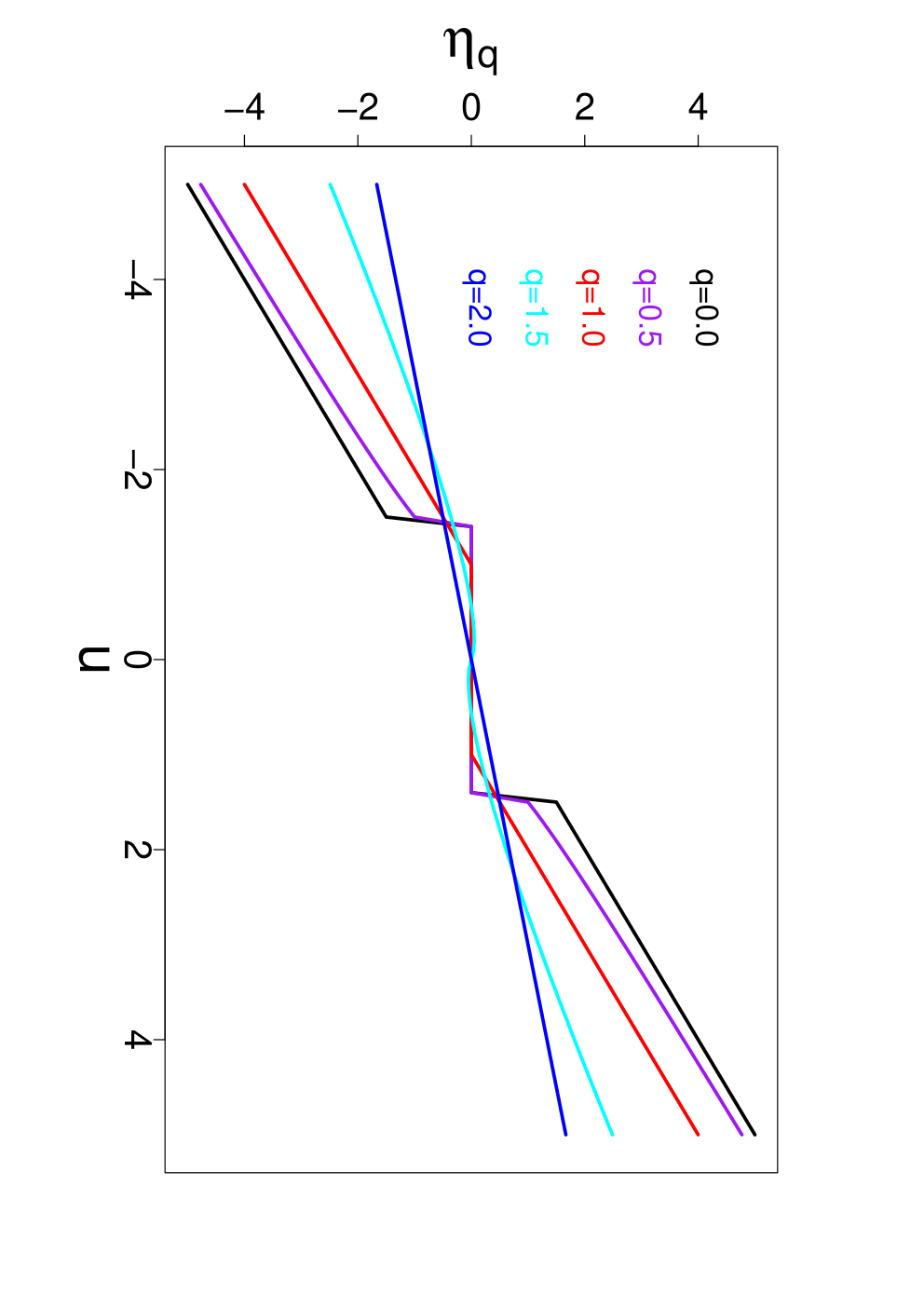
For a converging sequence of instances, we can define the function

where ${\bf z}\sim N(0,{\bf I}_{p\times p})$ is independent of $\mbox{\boldmath$\beta$}_{0}$. Notice that the function $\psi_{q}(\cdot,\cdot)$ depends implicitly on the law $p_{\beta_{0}}$.

Denote $\hat{\mbox{\boldmath$\beta$}}(\lambda,p)$ the LQLS estimator for instance $\{\mbox{\boldmath$\beta$}_{0}(p),{\bf w}(p)$, $\mbox{\boldmath$\Sigma$}(p),{\bf X}(p)\}$ with $\lambda\textgreater 0$ based on (2). Then the following proposition establishes the distributional limit of $(\hat{\mbox{\boldmath$\beta$}}(\lambda,p),\mbox{\boldmath$\beta$}_{0})$.

The derivation of this proposition is presented in the supplementary material using the replica method which is a non-rigorous technique invented in statistical physics to study the behavior of large magnetic and disordered systems. This method has been used to analyze the accuracy of $\hat{\mbox{\boldmath$\beta$}}(\lambda,p)$ for i.i.d. Gaussian ${\bf X}$, i.e. $\mbox{\boldmath$\Sigma$}={\bf I}_{p}$ in Rangan et al. 2009. Here we generalize it to arbitrary $\Sigma$.

The performance of LQLS estimator (2) depends on the choice of the threshold parameters $\lambda$. Any fair comparison between LQLS for different values of $q$ must take this fact into account. Consider a test point ${\bf x}_{0}\sim N(0,\mbox{\boldmath$\Sigma$})$ independent of the train data. For an estimator $\hat{\mbox{\boldmath$\beta$}}$ (a function of the training data ${\bf X},{\bf y}$), we define its prediction risk (or simply, risk) as

For $\mbox{\boldmath$\Sigma$}={\bf I}_{p}$, $R_{q}(\hat{\mbox{\boldmath$\beta$}}(\lambda))$ is equivalent to the MSE defined in Weng et al. 2016. Hence, it is important to pick $\lambda$ optimally by minimizing the prediction risk, i.e. $\lambda_{\star}=\text{argmin}_{\lambda}R_{q}(\hat{\mbox{\boldmath$\beta$}}(\lambda))$. This is equivalent to consider the following optimal thresholding policy

since $R_{q}(\hat{\mbox{\boldmath$\beta$}}(\lambda_{\star}))=\delta[\psi(\tau_{\star}^{2},\alpha_{\star}(\tau_{\star}))-\sigma^{2}_{w}]$. This enables us to focus the analysis on a single equation rather than two equations (12) and (13). The results we will present in the next two sections are mainly based on investigating the solution of the following fixed point equation

We consider the cases $0\leq q\textless 1$ and $1\textless q\leq 2$ separately.

When $0\leq q\textless 1$, the $L_{q}$ regularization has the nice property of creating coefficient sparsity because the generalized thresholding operation $\mbox{\boldmath$\eta$}_{q}({\bf v},\lambda)$ defined in (4) maps small values of ${\bf v}$ to zero. Also the smaller values of $q$ correspond to a preference for increasingly sparse solutions. However, the penalty term is not convex for $q\textless 1$ which makes solving the optimization problem much more difficult because the local minima may not be unique.

The difference between the regularization for $1\textless q\leq 2$ and the regularization for $0\leq q\textless 1$ is that the former is convex and its optimization problem has a unique global minimum. However, since its penalty is differentiable everywhere, it never leads to a coefficient been zero rather only minimizes it when $\lambda\neq 0$. Our first result is concerned with the first dominant term of the optimally tuned asymptotic prediction risk defined as $R_{q}(\tau_{\star},\sigma_{w})=\min_{\lambda}\frac{1}{p}\|\hat{\mbox{\boldmath$\beta$}}(\lambda)-\mbox{\boldmath$\beta$}_{0}\|_{\mbox{\boldmath$\Sigma$}}^{2}$ which is related to the phase transition curve for successful recovery.

Therefore, assume the error $\sigma_{w}^{2}$ equals zero, for $1\textless q\leq 2$ and any $\gamma\textgreater 0$, if $\delta\textgreater 1+\gamma$, then (2) succeeds in recovering $\beta$, while if $\delta\textless 1-\gamma$, (2) fails. The phase transition curve $\delta=1$ is independent of $\epsilon$, $q$, and the covariance structure of $\Sigma$. As pointed out by Zheng et al. 2017, phase transition analysis based on the first dominant term may lead to misleading conclusions in any practical setting where there is always error in the response variables. To study the impact of them, we need to conduct higher-order analysis of LQLS in the small-error regime in the expansion of prediction risk $R_{q}(\tau_{\star},\sigma_{w})$.

Our second result is concerned with the second dominant term of the optimally tuned MSE of LQLS when the number of response variables is larger than the number of predictors $p$, i.e. $\delta\textgreater 1$. The key is to characterize the convergence rate for $R_{q}(\tau_{\star},\sigma_{w})$ as $\sigma_{w}\rightarrow 0$.

The first term $\frac{\delta\sigma_{w}^{2}}{\delta-1}$ shows a notion of phase transition. For as $\sigma_{w}\rightarrow 0$, $R_{q}(\tau_{\star},\sigma_{w})=O(\sigma_{w}^{2})$, and will go to zero. For $\rho=0$, the second dominant term is the same as the one derived in Theorem 3.1 in Weng et al. 2018. The important facts of the second dominant term include: (1) it is negative; (2) its order is $\sigma_{w}^{2q}$; (3) its magnitude decreases with $\epsilon$ for fixed $q$ and $\rho$; (4) its magnitude decreases with $q$ for fixed $\epsilon$ and $\rho$; (5) its magnitude increases with $\rho$ for fixed $q$ and $\epsilon$. Facts (3) and (4) have been studied thoroughly in Weng et al. 2018. Our numerical studies in Section 5 focus on the verification of fact (5).

This section performs several numerical studies to evaluate the $R_{q}(\tau_{\star},\sigma_{w})$ of LQLS as a function of $\sigma_{w}$ for several different values of $q$ and $\rho$. Here we consider a block diagonal matrix $\Sigma$ with two-dimensional block $\left(\begin{array}[]{cc}1&\rho\\ \rho&1\end{array}\right)$. The equation can be decomposed into 2-dimensional blocks. Sections 5.1 and 5.2 study the performance of LQLS with $0\leq q\textless 1$ and $1\textless q\leq 2$ respectively.

$L_{q}$-regularized least square is one of the most popular schemes for recovering a high-dimensional sparse vector from low-dimensional measurements. This paper focuses on asymptotic behavior of LQLS estimators in the framework in which it is assumed that $p,n,k\rightarrow\infty$ while $n/p\rightarrow\delta$ and $k/p\rightarrow\epsilon$ are fixed. We first derive the distributional limit of LQLS estimators for nonstandard Gaussian design models where the row of design matrix ${\bf X}$ are drawn independently from distribution $N(0,\mbox{\boldmath$\Sigma$})$ with arbitrary $\Sigma$. Then we obtain an explicit characterization of the asymptotic risk by deriving its higher order expansion in the small-error regime. Our analysis is performed on both the convex case $1\textless q\leq 2$ and non-convex case $0\leq q\textless 1$. We conclude that the first order term does not depend on the covariance structure of $\Sigma$ and thus the phase transition curves are the same as the in the case of standard Gaussian design. This is different from the case $q=1$ in which the correlation can change the phase transition boundary if the signed pattern of signal is not symmetric. The second order term depends on the correlation and the explicit formulas are derived in both cases based on a simple two-dimensional block diagonal covariance model.

Note that part of our analysis is based on the replica method which are not fully rigorous yet. So far the rigorous work in this area mainly focuses on i.i.d. randomness. For example, the mean square error of LQLS for the case of $1\leq q\leq 2$ is characterized using Gordon’s lemma in Thrampoulidis et al. 2018 and AMP in Weng et al. 2018. For nonstandard Gaussian design models, $\mbox{\boldmath$\Sigma$}\neq I_{p\times p}$ the rigorous analysis for the case $q=1$ have been conducted recently Celentano et al. 2020 using Gordon’s comparison inequality and in Huang 2021 using AMP. Our next step is to derive the rigorous results for Proposition 1 for the case $1\textless q\leq 2$. The case $0\textless q\leq 1$ is more challenging because the penalty term is not convex and even in the i.i.d. case its rigorous results have not been established yet.

Our conclusion in this paper is based on higher-order analysis in small error region. It may not be applicable if the noisy error is large enough. As shown in Zheng et al. 2017, for large values of noise, the LASSO outperforms $L_{0}$-minimization and if $q_{1}\textgreater q_{2}$, then optimal $L_{q_{1}}$-minimization outperforms optimal $L_{q_{2}}$-minimization. Proposition 3 of Zheng et al. 2017 provides theoretical justification on this high-noise phenomenon. Another direction of our future research is to study the high-noise phenomenon of LQLS for nonstandard Gaussian design models.

This appendix outlines the proofs of the Propositions in the main text.

References

- Amelunxen et al. (2013) Amelunxen, D., M. Lotz, M. B. McCoy, and J. A. Tropp (2013). Living on the edge: phase transitions in convex programs with random data. Information and Inference: A Journal of the IMA 3, 224–294.
- Baddeley (1977) Baddeley, A. (1977). Integrals on a moving manifold and geometrical probability. Advances in Applied Probability 9(3), 588–603.
- Celentano et al. (2020) Celentano, M., A. Montanari, and Y. Wei (2020). The lasso with general gaussian designs with applications to hypothesis testing. arXiv, 10.48550/ARXIV.2007.13716.
- Chartrand and Staneva (2008) Chartrand, R. and V. Staneva (2008, may). Restricted isometry properties and nonconvex compressive sensing. Inverse Problems 24(3), 035020.
- Donoho (2006) Donoho, D. L. (2006). For most large underdetermined systems of linear equations the minimal -norm solution is also the sparsest solution. Communications on Pure and Applied Mathematics 59(6), 797–829.
- Donoho et al. (2011) Donoho, D. L., A. Maleki, and A. Montanari (2011, Oct). The noise-sensitivity phase transition in compressed sensing. IEEE Transactions on Information Theory 57(10), 6920–6941.
- Donoho and Tanner (2005) Donoho, D. L. and J. Tanner (2005). Sparse nonnegative solution of underdetermined linear equations by linear programming. Proceedings of the National Academy of Sciences 102(27), 9446–9451.
- Fu and Knight (2000) Fu, W. and K. Knight (2000). Asymptotics for lasso-type estimators. The Annals of Statistics 28(5), 1356 – 1378.
- Huang (2021) Huang, H. (2021). Lasso risk and phase transition under dependence. arXiv, 10.48550/ARXIV.2103.16035.
- Javanmard and Montanari (2014) Javanmard, A. and A. Montanari (2014, Oct). Hypothesis testing in high-dimensional regression under the gaussian random design model: Asymptotic theory. IEEE Transactions on Information Theory 60(10), 6522–6554.
- Kabashima et al. (2009) Kabashima, Y., T. Wadayama, and T. Tanaka (2009, sep). A typical reconstruction limit for compressed sensing based on -norm minimization. Journal of Statistical Mechanics: Theory and Experiment 2009(09), L09003.
- Ma et al. (2019) Ma, J., J. Xu, and A. Maleki (2019). Optimization-based amp for phase retrieval: The impact of initialization and regularization. IEEE Transactions on Information Theory 65(6), 3600–3629.
- Meinshausen and Bühlmann (2006) Meinshausen, N. and P. Bühlmann (2006). High-dimensional graphs and variable selection with the Lasso. The Annals of Statistics 34(3), 1436 – 1462.
- Mézard and Montanari (2009) Mézard, M. and A. Montanari (2009). Information, Physics, and Computation. Oxford Graduate Texts. OUP Oxford.
- Mezard et al. (1987) Mezard, M., G. Parisi, and M. Virasoro (1987). Spin Glass Theory and Beyond: An Introduction to the Replica Method and Its Applications. World Scientific Lecture Notes in Physics. World Scientific.
- Rangan et al. (2009) Rangan, S., V. Goyal, and A. K. Fletcher (2009). Asymptotic analysis of map estimation via the replica method and compressed sensing. In Y. Bengio, D. Schuurmans, J. Lafferty, C. Williams, and A. Culotta (Eds.), Advances in Neural Information Processing Systems, Volume 22. Curran Associates, Inc.
- Saab et al. (2008) Saab, R., R. Chartrand, and O. Yilmaz (2008). Stable sparse approximations via nonconvex optimization. In 2008 IEEE International Conference on Acoustics, Speech and Signal Processing, pp. 3885–3888.
- Saab and Özgür Yılmaz (2010) Saab, R. and Özgür Yılmaz (2010). Sparse recovery by non-convex optimization – instance optimality. Applied and Computational Harmonic Analysis 29(1), 30–48.
- Stojnic (2013) Stojnic, M. (2013). Lifting -optimization thresholds. arXiv, https://arxiv.org/abs/1306.3976.
- Thrampoulidis et al. (2018) Thrampoulidis, C., E. Abbasi, and B. Hassibi (2018). Precise error analysis of regularized -estimators in high dimensions. IEEE Transactions on Information Theory 64(8), 5592–5628.
- Wang et al. (2011) Wang, M., W. Xu, and A. Tang (2011). On the performance of sparse recovery via -minimization . IEEE Transactions on Information Theory 57(11), 7255–7278.
- Wang et al. (2020) Wang, S., H. Weng, and A. Maleki (2020). Which bridge estimator is the best for variable selection? The Annals of Statistics 48(5), 2791 – 2823.
- Wang et al. (2021) Wang, S., H. Weng, and A. Maleki (2021). Does SLOPE outperform bridge regression? Information and Inference: A Journal of the IMA 11(1), 1–54.
- Weng and Maleki (2019) Weng, H. and A. Maleki (2019). Low noise sensitivity analysis of -minimization in oversampled systems. Information and Inference: A Journal of the IMA 9(1), 113–155.
- Weng et al. (2018) Weng, H., A. Maleki, and L. Zheng (2018). Overcoming the limitations of phase transition by higher order analysis of regularization techniques. The Annals of Statistics 46(6A), 3099 – 3129.
- Weng et al. (2016) Weng, H., L. Zheng, A. Maleki, and X. Wang (2016). Phase transition and noise sensitivity of -minimization for . In 2016 IEEE International Symposium on Information Theory (ISIT), pp. 675–679.
- Zheng et al. (2017) Zheng, L., A. Maleki, H. Weng, X. Wang, and T. Long (2017). Does -minimization outperform -minimization? IEEE Transactions on Information Theory 63(11), 6896–6935.