Optimal performance of a tontine overlay subject to withdrawal constraints
Abstract
We consider the holder of an individual tontine retirement account, with maximum and minimum withdrawal amounts (per year) specified. The tontine account holder initiates the account at age 65, and earns mortality credits while alive, but forfeits all wealth in the account upon death. The holder desires to maximize total withdrawals, and minimize the expected shortfall, assuming the holder survives to age 95. The investor controls the amount withdrawn each year and the fraction of the investments in stocks and bonds. The optimal controls are determined based on a parametric model fitted to almost a century of market data. The optimal control algorithm is based on dynamic programming and solution of a partial integro differential equation (PIDE) using Fourier methods. The optimal strategy (based on the parametric model) is tested out of sample using stationary block bootstrap resampling of the historical data. In terms of an expected total withdrawal, expected shortfall (EW-ES) efficient frontier, the tontine overlay greatly outperforms an optimal strategy (without the tontine overlay), which in turn outperforms a constant weight strategy with withdrawals based on the ubiquitous four per cent rule.
Keywords: tontine, decumulation, expected shortfall, optimal stochastic control
JEL codes: G11, G22
AMS codes: 91G, 65N06, 65N12, 35Q93
1 Introduction
It is now commonplace to observe that defined benefit (DB) plans are disappearing. A recent OECD study (OECD 2019) observes that less than 50% of pension assets in 2018 were held in DB plans in over 80% of countries reporting. Of course, the level of assets in defined contribution (DC) plans is a lagging indicator, since historically, many employees were covered by traditional DB plans. These traditional DB plans still have a sizeable share of pension assets, simply because these plans have accumulated contributions over a longer period of time.
Consider the typical case of a DC plan investor upon retirement. Assuming that the investor has managed to accumulate a reasonable amount in her DC plan, the investor now faces the problem of determining a decumulation strategy, i.e. how to invest and spend during retirement. It is often suggested that retirees should purchase annuities, but this is an unpopular strategy (Peijnenburg et al. 2016). MacDonald et al. 2013 note that this avoidance of annuities can be entirely rational.
A major concern of DC plan investors during the decumulation phase is, naturally, running out of savings. Possibly the most widely cited benchmark strategy is the 4% rule (Bengen 1994). This rule posits a retiree who invests in a portfolio of 50% stocks and 50% bonds, rebalanced annually, and withdraws 4% of the original portfolio value each year (adjusted for inflation). This strategy would have never depleted the portfolio over any rolling thirty year historical period tested by Bengen on US data. This rule has been revisited many times. For example, Guyton and Klinger 2006 suggest several heuristic modifications involving withdrawal amounts and investment strategies.
Another approach has been suggested by Waring and Siegel 2015, which they term an Annually Recalculated Virtual Annuity (ARVA) strategy. The idea here is that the amount withdrawn in any given year should be based on the cash flows from a virtual (i.e. theoretical) fixed term annuity that could be purchased using the existing value of the portfolio. In this case, the DC plan can never run out of cash, but the withdrawal amounts can become arbitrarily small.
Turning to asset allocation strategies, Irlam 2014 used dynamic programming methods to conclude that deterministic (i.e. glide path) allocation strategies are sub-optimal. Of course, the asset allocation strategy and the withdrawal strategy are intimately linked. A more systematic approach to the decumulation problem involves formulating decumulation strategies as a problem in optimal stochastic control. The objective function for this problem involves a measure of risk and reward, which are, of course, conflicting measures. Forsyth 2022b uses the withdrawal amount and the asset allocation (fraction in stocks and bonds) as controls. The measure of reward is the total (real) accumulated withdrawal amounts over a thirty year period. The withdrawal amounts have minimum and maximum constraints, hence there is a risk of depleting the portfolio. The measure of risk is the expected shortfall at the 5% level, of the (real) value of the portfolio at the thirty year mark. Utilizing both withdrawal amounts and asset allocation as controls considerably reduces the risk of portfolio depletion compared to fixed allocation or fixed withdrawal strategies.
A recent innovation in retirement planning involves the use of modern tontines (Donnelly et al. 2014; Donnelly 2015; Milevsky and Salisbury 2015; Fullmer 2019; Weinert and Grundi 2021; Winter and Planchet 2022; Milevsky 2022). In a tontine, the investor makes an irrevocable investment in a pooled fund for a fixed time frame. If the investor dies during the time horizon of the investment, the investor’s portfolio is divided amongst the remaining (living) members of the fund. If the investor survives until the end of the time horizon, then she will earn mortality credits from those members who have passed away. Unlike an annuity, there are no guaranteed cash flows, since typically the funds are invested in risky assets. Since there are no guarantees, the expected cash flows from a tontine are larger than for an annuity (with the same initial investment). Some authors have argued that the annuity puzzle should be replaced by the tontine puzzle, i.e. since tontines seem to very efficient products for pooling longevity risk, it is puzzling that the tontine market is still in its infancy (Chen and Rach 2022). Pooled funds with tontine characteristics have been in use for some time.11 1 The variable annuity funds offered by TIAA https://www.tiaa.org/public/, the University of British Columbia pension plan https://faculty.pensions.ubc.ca/, and the Australian Q-super fund https://qsuper.qld.gov.au/ can all be viewed as having tontine characteristics. However, the Q-super fund takes the approach of averaging mortality credits over the entire pool, giving age independent mortality credits, which would appear to violate actuarial fairness. https://i3-invest.com/2021/04/behind-qsupers-retirement-design/ The Q-super fund is perhaps more properly termed a collective defined contribution (CDC) fund. CDCs https://www.ft.com/content/10448b2c-1141-4d2e-943c-70cce2caec52 have been criticized for lack of transparency and fairness. We should also mention that retail investors may find the concept of a tontine appealing, simply due to the peer-to-peer model for managing longevity risk, which is also consistent with the trend towards financial disintermediation.22 2 See van Benthem et al. 2018 for an experiment with setting up a tontine using blockchain techniques. However, tontines may also require changes to existing legislation in some jurisdictions (MacDonald et al. 2021). There have also been suggestions for government management of tontine accounts (Fullmer and Forman 2022; Fuentes et al. 2022). The attractiveness of tontines, from a behavioral finance perspective, is discussed in Chen et al. 2021. For an overview comparison of modern tontines to existing decumulation products, we refer the reader to Bar and Gatzert 2022.
Our focus in this article is on individual tontine accounts (Fullmer 2019), whereby the investor has full control over the asset allocation in her account. We also allow the investor to control the withdrawal amount from the account, subject to maximum and minimum constraints. Usually it is suggested that withdrawal amounts from a tontine account cannot be increased, to avoid moral hazard issues.33 3 An obvious case would be if an investor was given a medical diagnosis with a high probability of a poor outcome, at which point the investor would withdraw all remaining funds in her account. However, we view the maximum withdrawal as the desired withdrawal, allowing temporary reductions in withdrawals to minimize sequence of return risk and probability of ruin.
Consider an investor whose objective function uses reward as measured by total expected accumulated (real) withdrawals (EW) over a thirty year period. As a measure of risk, the investor uses the expected shortfall (ES) of the portfolio at the thirty year point. In this work, we define the expected shortfall as the mean of the worst 5% of the outcomes at year thirty. The investor’s controls are the amount withdrawn each year, and the allocations to stocks and bonds. The investor follows an optimal strategy to maximize this objective function.
Alternatively, the investor can use the same objective function, with the same controls, but this time add a tontine overlay (i.e. the investor is part of a pooled tontine). The investor has control over the withdrawals (subject of course to the same maximum and minimum constraints), and the allocation strategy.
Of course, we expect that the investor who uses the tontine overlay would achieve a better result than without the overlay, due to the mortality credits earned (we assume that the investor does not pass away during the thirty year investment horizon). However, this does not come without a cost. If the investor passes away, then her portfolio is forfeited.
Therefore, the investor must be compensated with a sizeable reduction in the risk of portfolio depletion, compared to the no-tontine overlay case. The objective of this article is to quantify this reduction, assuming optimal policies are followed in each case.
More precisely, we consider a 65-year old retiree, who can invest in a portfolio consisting of a stock index and a bond index, with yearly withdrawals, and rebalancing. The investor desires to maximize the multi-objective function in terms of the risk and reward measures described above, evaluated at the thirty year horizon (i.e. when the investor is 95).
We calibrate a parametric stochastic model for real (i.e. inflation adjusted) stock and bond returns, to almost a century of market data. We then solve the optimal stochastic control problem numerically, using dynamic programming. Robustness of the controls is then tested using block bootstrap resampling of the historical data.
Our main conclusion is that for a reasonable specification of acceptable tail risk (i.e. expected shortfall), the expected total cumulative withdrawals (EW) are considerably larger with the tontine overlay, compared to without the overlay. This conclusion holds even if the tontine overlay has fees of the order of 50-100 bps per year. Consequently, if the retiree has no bequest motive, and is primarily concerned with the risk of depleting her account, then a tontine overlay is an attractive solution.
It is also interesting to note that the optimal control for the withdrawal amount is (to a good approximation) a bang-bang control, i.e. it is only optimal to withdraw either the maximum or minimum amount in any year. The allocation control essentially starts off with 40-50% allocation to stocks. The median allocation control then rapidly reduces the fraction in equities to a very small amount after years. The median withdrawal control starts off at the minimum withdrawal amount, and then rapidly increases withdrawals to the maximum after years. The precise timing of the switch from minimum withdrawal to maximum withdrawal is simply a function of how much depletion risk (ES) the investor is prepared to take.
2 Overview of Individual Tontine Accounts
2.1 Intuition
We give a brief overview of modern tontines in this section. We restrict attention to the case of an individual tontine account (Fullmer 2019), which is a constituent of a perpetual tontine pool. Consider a pool of investors, who are alive at time . Let be the balance in the portfolio of investor at time . In a tontine, if investor participates in a tontine pool in time interval , and investor dies in that interval, then her portfolio is forfeited and given to the surviving members of the pool in the form of mortality credits (gains). Suppose that the probability that dies in is . Let the tontine gain (mortality credit) for investor , for the period , paid out at time , be denoted by . The tontine will be a fair game if, for each player , the expected gain from participating in the tontine is zero,
| (2.1) |
and solving for the tontine gain gives
| (2.2) |
For notational convenience, we define the tontine gain rate at for investor as
| (2.3) |
In our optimal control formulation, we will typically drop the superscript from equation (2.3),
| (2.4) |
since we will consider a given investor with conditional mortality probability of in .
2.2 Group Gain
Consider tontine members who are are alive at . Let
| (2.5) |
where is the expectation operator. Note that the total tontine gain for all members at is
| Total Tontine Gains | (2.6) | ||||
and that the total amount forfeited by members who have died in is
| Total Forfeited | (2.7) |
Then
| (2.8) |
implying that the expected total tontine gain is balanced by the expected total amount forfeited.
In practice, of course, the expected number of deaths in period may not be equal to the actual number of deaths. To compensate for this, a practical implementation method has been suggested in (Sabin and Forman 2016; Denuit and Vernic 2018; Fullmer and Sabin 2019; Fullmer 2019; Winter and Planchet 2022). Denote the realized group gain at by
| (2.9) |
Observe that the values of in equation (2.9) are the realized values, not expectations. The actual tontine gain (mortality credit) earned by investor (assuming investor is alive at ) is then
| (2.10) |
Essentially, we are scaling equation (2.2) by the factor , which ensures that the the total amount forfeited by the observed deaths in is exactly equal to the total mortality credits disbursed to the survivors. In the following, we will refer to as the actual mortality gain, while will be termed the nominal tontine gain.
Remark 2.1 ().
Note that equation (2.9) is undefined if all members die in . We assume that the tontine is large (in terms of members) and perpetual, i.e. open to new members, so that the probability of all members dying is negligible. For mathematical completeness, we can suppose that if all members die in , we collapse the tontine, and distribute all remaining account values to the estates of members .
While use of equation (2.10) looks like a reasonable approach, it turns out that this is not strictly fair in the actuarial sense, i.e. there is some bias that favors some members over others. Informally, this bias exists since the total amount forfeited in a period depends on the binary state of each member of the pool, i.e. alive or dead.44 4 This is illustrated in Winter and Planchet 2022, using an example with pool consisting of a large number of young investors (with small individual portfolios), and a single elderly member with a large portfolio. The elderly member effectively subsidizes the younger members. Sabin and Forman 2016 show that the bias is negligible under the following conditions
Condition 2.1 (Small bias condition).
Suppose that the following conditions hold
- (a)
-
the pool of participants in the tontine is sufficiently large;
- (b)
-
the expected amount forfeited by all members is large compared to any member’s nominal gain, i.e.
(2.11)
then the bias is negligibly small (Sabin and Forman 2016).
Condition (2.11) is essentially a diversification requirement: no member of the pool has an abnormally large share of the total pool capital. In addition, of course, if the pool is sufficiently large, then the actual number of deaths in will converge to the expected number of deaths.
Note that it does not matter what investment strategy is followed by any given investor in period . Each investor can choose whatever policy they like, since only the observed final portfolio value at matters. Somewhat counterintuitively, is very close to unity, even if the participants in the tontine pool are very heterogeneous, i.e. with different ages, genders, invested amounts, and asset allocations (assuming Condition 2.1 holds).
In Fullmer and Sabin 2019, simulations were carried out to determine the magnitude of the volatility of under practical sizes of tontine pools. Given a tontine pool of 15,000 members, with varying ages, initial capital, and randomly assigned investment policies (i.e. the bond/stock split), the simulations showed that and that the standard deviation was about . This standard deviation at each actually resulted in a smaller effect over a long term (assuming that the tontine member lived long enough). This is simply because everybody dies eventually, so that if fewer deaths than expected are observed in a year, then more deaths will be observed in later years, and vice versa.
In the following, we will assume that the pool is sufficiently large and that it satisfies the diversity condition (2.11), so that there is no error in assuming that , i.e we will assume that the nominal tontine gain is the actual tontine gain. As a sanity check, we also carry out a test whereby we simulate the effect of randomly varying , based on the statistics of the simulations in Fullmer and Sabin 2019. Our results show that effect of randomness in can be safely ignored for a reasonably sized tontine pool. To be more precise here, we will modify equation (2.4) so that
| (2.12) |
for a numerical example showing the effects of randomness of , in Monte Carlo simulations. Our computation of the optimal strategy will always assume .
2.3 Variable withdrawals
We will allow the individual tontine member to withdraw variable amounts, subject to minimum and maximum constraints. We remind the reader that if a tontine pool is strictly actuarially fair, then, in theory, there are no constraints on withdrawals and injections of cash (Braughtigam et al. 2017).
However, in practice, since pools are finite sized, heterogeneous, and mortality credits are not distributed at infinitesimal intervals, we do not allow arbitrarily large withdrawals. This avoids moral hazard issues.
Since we have a minimum withdrawal amount in each time period, there is a risk of running out of cash. We assume that if the tontine member’s account becomes negative, than all trading in this account ceases, and debt accumulates at the borrowing rate. In practice, once the tontine account becomes zero, the retiree has to fund expenses from another source. We implicitly assume that the tontine member has other assets which can be used to fund this minimum consumption level (e.g. real estate). Of course, we aim to make this a very improbable event. In fact, this is the reason why we allow variable withdrawals. We can regard the upper bound on the withdrawals as the desired consumption level, but we allow the tontine member to reduce (hopefully only temporarily) their withdrawals, to minimize risk of depletion of their tontine account.
2.4 Money back guarantees
In practice, we observe that many tontine funds offer a money back guarantee.55 5 https://qsuper.qld.gov.au/ This is usually specified as a return of the initial (nominal) investment less any withdrawals (if the sum is non-negative) at the time of death. We do not consider such guarantees in this work, focusing on the pure tontine aspect, which has no guarantees, and presumably the highest possible expected total withdrawals. A money back guarantee would have to be hedged, which would reduce returns. In practice, this guarantee could be priced separately, and added as overlay to the tontine investment if desired.
2.5 Survivor Benefits
Many DB plans have survivor benefits which are received by a surviving spouse. A typical case would involve the surviving spouse receiving of the yearly pension after the DB plan holder dies.
Consider the following case of a male, same-sex couple, both of whom are exactly the same age. As an extreme case, suppose the survivor benefit is 100% of the tontine cash flows, which continue until the survivor dies. From the CPM2014 table from the Canadian Institute of Actuaries66 6 www.cia-ica.ca/docs/default-source/2014/214013e.pdf, the probability that an 85-year old Canadian male dies before reaching the age of 86 is about . Assuming that the mortality probabilities are independent for both spouses, then the probability that both 85-year old spouses die before reaching age , conditional on both living to age is . The tontine gain rate per year (from equation (2.3)) is
| tontine gain rate | (2.13) |
We will assume in our numerical examples that the base case fee charged for managing the tontine is bps per year. This means that, net of fees, there are essentially no tontine gains for our hypothetical couple, for the first 20 years of retirement, which is surely undesirable. Once one of the partners passes away, the tontine gain rate will, of course, take a jump in value.
As another extreme case, suppose that the surviving spouse receives of the tontine cash flows. In this case, the total cash flows accruing this couple are exactly the same as dividing the original total wealth into two, and then having each spouse invest in their own individual tontine.
It is possible to determine the distribution of the cash flows for a survivor benefit which is intermediate to these edge cases. However, this requires additional state variables in our optimal control problem, and is probably best tackled using a machine learning approach (Li and Forsyth 2019; Ni et al. 2022). We will leave this case for future work, and focus attention on the individual tontine case, with no survivor benefit. Note that in the tontine context, survivor benefits are typically provided by a separate insurance overlay.77 7 https://i3-invest.com/2021/04/behind-qsupers-retirement-design/
3 Formulation
We assume that the investor has access to two funds: a broad market stock index fund and a constant maturity bond index fund.
The investment horizon is . Let and respectively denote the real (inflation adjusted) amounts invested in the stock index and the bond index respectively. In general, these amounts will depend on the investor’s strategy over time, as well as changes in the real unit prices of the assets. In the absence of an investor determined control (i.e. cash withdrawals or rebalancing), all changes in and result from changes in asset prices. We model the stock index as following a jump diffusion.
In addition, we follow the usual practitioner approach and directly model the returns of the constant maturity bond index as a stochastic process, see for example Lin et al. 2015; MacMinn et al. 2014. As in MacMinn et al. 2014, we assume that the constant maturity bond index follows a jump diffusion process as well.
Let , i.e. is the instant of time before , and let be a random number representing a jump multiplier. When a jump occurs, . Allowing for jumps permits modelling of non-normal asset returns. We assume that follows a double exponential distribution (Kou 2002; Kou and Wang 2004). If a jump occurs, is the probability of an upward jump, while is the chance of a downward jump. The density function for is
| (3.1) |
We also define
| (3.2) |
In the absence of control, evolves according to
| (3.3) |
where is the (uncompensated) drift rate, is the volatility, is the increment of a Wiener process, is a Poisson process with positive intensity parameter , and are i.i.d. positive random variables having distribution (3.1). Moreover, , , and are assumed to all be mutually independent.
Similarly, let the amount in the bond index be . In the absence of control, evolves as
| (3.4) |
where the terms in equation (3.4) are defined analogously to equation (3.3). In particular, is a Poisson process with positive intensity parameter , and has distribution
| (3.5) |
and . , , and are assumed to all be mutually independent. The term in equation (3.4) represents the extra cost of borrowing (the spread).
The diffusion processes are correlated, i.e. . The stock and bond jump processes are assumed mutually independent. See Forsyth 2020b for justification of the assumption of stock-bond jump independence.
We define the investor’s total wealth at time as
| (3.6) |
We impose the constraints that (assuming solvency) shorting stock and using leverage (i.e. borrowing) are not permitted. In the event of insolvency (due to withdrawals), the portfolio is liquidated, trading ceases and debt accumulates at the borrowing rate.
4 Notational Conventions
Consider a set of discrete withdrawal/rebalancing times
| (4.1) |
where we assume that is constant for simplicity. To avoid subscript clutter, in the following, we will occasionally use the notation and . Let the inception time of the investment be . We let be the set of withdrawal/rebalancing times, as defined in equation (4.1). At each rebalancing time , , the investor (i) withdraws an amount of cash from the portfolio, and then (ii) rebalances the portfolio. At , the portfolio is liquidated and no cash flow occurs. For notational completeness, this is enforced by specifying .
In the following, given a time dependent function , then we will use the shorthand notation
| ; | (4.2) |
Let
| (4.3) |
We assume that a tontine fee of per unit time is charged at , based on the total portfolio value at , after tontine gains but before withdrawals. Recalling the definition of tontine gain rate in equation (2.4), we modify this definition to enforce no tontine gain at ,
| (4.4) |
Then, is given by
| (4.5) |
where we recall that and . With some abuse of notation, we define
| (4.6) |
as the total portfolio value, after tontine gains and tontine fees, the instant before withdrawals and rebalancing at .
Typically, DC plan savings are held in a tax advantaged account, with no taxes triggered by rebalancing. With infrequent (e.g. yearly) rebalancing, we also expect other transaction costs, apart from the tontine fees, to be small, and hence can be ignored. It is possible to include transaction costs, but at the expense of increased computational cost (van Staden et al. 2018).
We denote by , , the multi-dimensional controlled underlying process, and by the realized state of the system. Let the rebalancing control be the fraction invested in the stock index at the rebalancing date , i.e.
| (4.7) |
Let the withdrawal control be the amount withdrawn at time , i.e. . Formally, the controls depend on the state of the investment portfolio, before the rebalancing occurs, i.e. , and , , where is the set of rebalancing times.
However, it will be convenient to note that in our case, we find the optimal control amongst all strategies with constant wealth (after withdrawal of cash). Hence, with some abuse of notation, we will now consider to be function of wealth after withdrawal of cash
| (4.8) |
Note that the control for depends only . Since , then it follows that
| (4.9) |
which we discuss further in Section 7.
A control at time , is then given by the pair where the notation denotes that the control is a function of the state.
Let represent the set of admissible values of the controls . We impose no-shorting, no-leverage constraints (assuming solvency). We also impose maximum and minimum values for the withdrawals. We apply the constraint that in the event of insolvency due to withdrawals (), trading ceases and debt (negative wealth) accumulates at the appropriate borrowing rate of return (i.e. a spread over the bond rate). We also specify that the stock assets are liquidated at .
More precisely, let be the wealth after withdrawal of cash, and be the total wealth before withdrawals (but after fees and tontine cash flows), then define
| (4.10) | |||||
| (4.11) |
The rather complicated expression in equation (4.10) imposes the assumption that, as wealth becomes small, the retiree (i) tries to avoid insolvency as much as possible and (ii) in the event of insolvency, withdraws only .
The set of admissible values for , can then be written as
| (4.13) |
For implementation purposes, we have written equation (4.13) in terms of the wealth after withdrawal of cash. However, we remind the reader that since , the controls are formally a function of the state before the control is applied.
The admissible control set can then be written as
| (4.14) |
An admissible control , where is the admissible control set, can be written as,
| (4.15) |
We also define as the tail of the set of controls in , i.e.
| (4.16) |
For notational completeness, we also define the tail of the admissible control set as
| (4.17) |
so that .
5 Risk and Reward
5.1 Risk: Definition of Expected Shortfall (ES)
Let be the probability density function of wealth at . Suppose
| (5.1) |
i.e. Pr. We can interpret as the Value at Risk (VAR) at level 88 8 In practice, the negative of is often the reported VAR.. The Expected Shortfall (ES) at level is then
| (5.2) |
which is the mean of the worst fraction of outcomes. Typically . The definition of ES in equation (5.2) uses the probability density of the final wealth distribution, not the density of loss. Hence, in our case, a larger value of ES (i.e. a larger value of average worst case terminal wealth) is desired. The negative of ES is commonly referred to as Conditional Value at Risk (CVAR).
Define . Given an expectation under control , , as noted by Rockafellar and Uryasev 2000, can be alternatively written as
| (5.3) |
The admissible set for in equation (5.3) is over the set of possible values for .
The notation emphasizes that is as seen at . In other words, this is the pre-commitment . A strategy based purely on optimizing the pre-commitment value of at time zero is time-inconsistent, hence has been termed by many as non-implementable, since the investor has an incentive to deviate from the time zero pre-commitment strategy at . However, in the following, we will consider the pre-commitment strategy merely as a device to determine an appropriate level of in equation (5.3). If we fix , then this strategy is the induced time consistent strategy (Strub et al. 2019), hence is implementable. We delay further discussion of this subtle point to Appendix A.
5.2 A measure of reward: expected total withdrawals (EW)
We will use expected total withdrawals as a measure of reward in the following. More precisely, we define EW (expected withdrawals) as
| (5.4) |
Note that there is no discounting term in equation (5.4) (recall that all quantities are real, i.e. inflation adjusted). It is straightforward to introduce discounting, but we view setting the real discount rate to zero to be a reasonable and conservative choice. See Forsyth 2022b for further comments.
6 Problem EW-ES
Since expected withdrawals (EW) and expected shortfall (ES) are conflicting measures, we use a scalarization technique to find the Pareto points for this multi-objective optimization problem. Informally, for a given scalarization parameter , we seek to find the control that maximizes
| (6.1) |
More precisely, we define the pre-commitment EW-ES problem problem in terms of the value function
| (6.2) | |||||
| subject to | (6.3) |
Note that we have added the extra term to equation (6.2). If we have a maximum withdrawal constraint, and if as , the controls become ill-posed. In this fortunate state for the investor, we can break the investment policy ties by setting , which will force investments in bonds, while if , then this will force investments into stocks. Choosing ensures that this term only has an effect if and . See Forsyth 2022b for more discussion of this.
Interchange the in equation (6.2), so that value function can be written as
Noting that the inner supremum in equation () is a continuous function of , and noting that the optimal value of in equation () is bounded99 9 This is the same as noting that a finite value at risk exists. This easily shown, assuming , since our investment strategy uses no leverage and no-shorting., then define
We refer the reader to Forsyth 2020a for an extensive discussion concerning pre-commitment and time consistent ES strategies. We summarize the relevant results from that discussion in Appendix A.
7 Formulation as a Dynamic Program
We use the method in Forsyth 2020a to solve problem (). We write equation () as
| (7.1) |
where the auxiliary function is defined as
| (7.2) | |||||
| subject to | (7.3) | ||||
We have now decomposed the original problem () into two steps
- •
For given initial cash , and a fixed value of , solve problem (7.2) using dynamic programming to determine .
- •
Solve problem () by maximizing over
(7.4)
7.1 Dynamic Programming Solution of Problem (7.2)
We give a brief overview of the method described in detail in (Forsyth 2022b). Apply the dynamic programming principle to
| (7.5) | |||||
For computational purposes, we define
| (7.6) |
Equation (7.5) now becomes
| (7.7) | |||||
This approach effectively replaces a two dimensional optimization for , to two sequential one dimensional optimizations. From equations (7.6-7.7), it is clear that the optimal pair is such that
| (7.8) | |||||
In other words, the optimal withdrawal control is only a function of total wealth (after tontine gains and fees) before withdrawals. The optimal control is a function only of total wealth after withdrawals, tontine gains, and fees.
At , we have
| (7.9) |
At points in between rebalancing times, i.e. , the usual arguments (from SDEs (3.3-3.4), and Forsyth 2022b) give
| (7.10) |
In case of insolvency1010 10 Insolvency can only occur due to the minimum withdrawals specified.
| (7.11) |
It will be convenient, for computational purposes, to re-write equation (7.11) in terms of debt when . Now let in equation (7.11) to give
| (7.12) |
Note that equation (7.12) is now amenable to a transformation of the form since , which is required when using a Fourier method (Forsyth and Labahn 2019; Forsyth 2022b) to solve equation (7.12).
After rebalancing, if , then cannot become negative, since is a barrier in equation (7.11). However, can become negative after withdrawals, in which case remains in the state , where equation (7.12) applies, unless there is an injection of cash to move to a state with . The terminal condition for equation (7.12) is
| (7.13) |
A brief overview of the numerical algorithms is given in Appendix B, along with a numerical convergence verification.
8 Data
We use data from the Center for Research in Security Prices (CRSP) on a monthly basis over the 1926:1-2020:12 period.1111 11 More specifically, results presented here were calculated based on data from Historical Indexes, ©2020 Center for Research in Security Prices (CRSP), The University of Chicago Booth School of Business. Wharton Research Data Services (WRDS) was used in preparing this article. This service and the data available thereon constitute valuable intellectual property and trade secrets of WRDS and/or its third-party suppliers. Our base case tests use the CRSP US 30 day T-bill for the bond asset and the CRSP value-weighted total return index for the stock asset. This latter index includes all distributions for all domestic stocks trading on major U.S. exchanges. All of these various indexes are in nominal terms, so we adjust them for inflation by using the U.S. CPI index, also supplied by CRSP. We use real indexes since investors funding retirement spending should be focused on real (not nominal) wealth goals.
We use the threshold technique (Mancini 2009; Cont and Mancini 2011; Dang and Forsyth 2016) to estimate the parameters for the parametric stochastic process models. Since the index data is in real terms, all parameters reflect real returns. Table 8.1 shows the results of calibrating the models to the historical data. The correlation is computed by removing any returns which occur at times corresponding to jumps in either series, and then using the sample covariance. Further discussion of the validity of assuming that the stock and bond jumps are independent is given in Forsyth 2020b.
| CRSP | |||||||
|---|---|---|---|---|---|---|---|
| 0.08912 | 0.1460 | 0.3263 | 0.2258 | 4.3625 | 5.5335 | 0.08420 | |
| 30-day T-bill | |||||||
| 0.0046 | 0.0130 | 0.5053 | 0.3958 | 65.801 | 57.793 | 0.08420 |
Remark 8.1 (Choice of 30-day T-bill for the bond index).
It might be argued that the bond index should hold longer dated bonds, e.g. ten-year treasuries, which would allow the investor to harvest the term premium. Long term bonds have enjoyed high real returns over the last thirty years, due to decreasing real interest rates during that time period. However, it is unlikely that this will continue to be true in the next thirty years. Hatch and White 1985 study the real returns of equities, short term T-bills, and long term corporate and government bonds, over the period 1950-1983, and conclude that, in both Canada and the US, only equities and short term T-bills had non-negative real returns. Inflation (both US and Canada) averaged about 4.75% per year over the period 1950-1983. If one imagines that the next thirty years will be a period with inflationary pressures, then this suggests that the defensive asset should be short term T-bills. However, there is nothing in the methodology in this paper which prevents us from using other underlying bonds in the bond index.
9 Historical Market
We compute and store the optimal controls based on the parametric model (3.3-3.4) as for the synthetic market case. However, we compute statistical quantities using the stored controls, but using bootstrapped historical return data directly. We remind the reader that all returns are inflation adjusted. We use the stationary block bootstrap method (Politis and Romano 1994; Politis and White 2004; Patton et al. 2009; Cogneau and Zakalmouline 2013; Dichtl et al. 2016; Cavaglia et al. 2022; Simonian and Martirosyan 2022; Anarkulova et al. 2022). A key parameter is the expected blocksize. Sampling the data in blocks accounts for serial correlation in the data series. We use the algorithm in Patton et al. 2009 to determine the optimal blocksize for the bond and stock returns separately, see Table 9.1. We use a paired sampling approach to simultaneously draw returns from both time series. In this case, a reasonable estimate for the blocksize for the paired resampling algorithm would be about years. We will give results for a range of blocksizes as a check on the robustness of the bootstrap results. Detailed pseudo-code for block bootstrap resampling is given in Forsyth and Vetzal 2019.
| Data series | Optimal expected |
|---|---|
| block size (months) | |
| Real 30-day T-bill index | 50.6 |
| Real CRSP value-weighted index | 3.42 |
10 Investment Scenario
Table 10.1 shows our base case investment scenario. We will use thousands of dollars as our units of wealth in the following. For example, a withdrawal of per year corresponds to per year (all values are real, i.e. inflation adjusted), with an initial wealth of (). This would correspond to the use of the four per cent rule (Bengen 1994). Our base case scenario assumes a fee of 50 bps per year. We refer to Chen et al. 2021 for a discussion of tontine fees.
As a motivating example, we consider a 65-year old Canadian retiree who has a pre-retirement salary of $100,000 per year, with $1,000,000 in a DC savings account. Government benefits are assumed to amount to about $20,000 per year (real). The retiree wishes the DC plan to generate at least $40,000 per year (real), so that the DC plan and government benefits replace 60% of pre-retirement income. We assume that the retiree owns mortgage-free real estate worth about $400,000. In an act of mental accounting, the retiree plans to use the real estate as a longevity hedge, which could be monetized using a reverse mortgage. In the event that the longevity hedge is not needed, the real-estate will be a bequest. Of course, the retiree would like to withdraw more than $40,000 per year from the DC plan, but has no use for withdrawals greater than $80,000 per year. We make the further assumption that the real-estate holdings can generate $200,000 through a reverse mortgage. Hence, as a rough rule of thumb, any expected shortfall at years greater than is an acceptable level of risk.
Our view that personal real estate is not fungible with investment assets (unless investment assets are depleted) is consistent with the behavioral life cycle approach originally described in Shefrin and Thaler 1988 and Thaler 1990. In this framework, investors divide their wealth into separate “mental accounts” containing funds intended for different purposes such as current spending or future need.
We take the view of a 65-year old retiree, who wants to maximize her total withdrawals, and minimize the risk of running out of savings, assuming that she lives to the age of 95. We also assume that the retiree has no bequest motive.
Recall that Bengen 1994 attempted to determine a safe real withdrawal rate, and constant allocation strategy, such that the probability of running out of cash after 30 years of retirement was small. In other words, Bengen 1994 maximized total withdrawals over a 30 year period, assuming that the retiree survived for the entire 30 years. This is, of course, a conservative assumption.
In our case, we are essentially answering the same question. The key difference here is that we (i) allow for dynamic asset allocation, (ii) allow variable withdrawals (within limits) and (iii) assume a tontine overlay.
| Retiree | 65-year old Canadian male |
|---|---|
| Tontine Gain | equation (2.2) |
| Group Gain ( see equation (2.12 ) ) | 1.0 |
| Mortality table | CPM 2014 |
| Investment horizon (years) | 30.0 |
| Equity market index | CRSP Cap-weighted index (real) |
| Bond index | 30-day T-bill (US) (real) |
| Initial portfolio value | 1000 |
| Cash withdrawalrebalancing times | |
| Maximum withdrawal (per year) | |
| Minimum withdrawal (per year) | |
| Equity fraction range | |
| Borrowing spread | 0.02 |
| Rebalancing interval (years) | 1.0 |
| (EW-ES) | .05 |
| Fees ( see equation (4.5) ) | 50 bps per year |
| Stabilization ( see equation (6.2) ) | |
| Market parameters | See Table 8.1 |
11 Constant Withdrawal, Constant Equity Fraction.
As a preliminary example, in this section we present results for the scenario in Table 10.1, except that a constant withdrawal of per year is specified, along with a constant weight in stocks at each rebalancing date.
Table 11.1 gives the results for various values of the constant weight equity fraction, in the synthetic market. The best result1212 12 Recall that is defined in terms of the left tail mean of final wealth (not losses) hence a larger value is preferred. for (the largest value) occurs at the rather low constant equity weight of , with an . Table 11.2 gives similar results, this time using bootstrap resampling of the historical data (the historical market). This time, the best value of occurs for a constant equity fraction of . Consequently, in both the historical and synthetic market, the constant weight, constant withdrawal strategy fails to meet our risk criteria of .
These simulations indicate that there is significant depletion risk for the constant withdrawal, constant weight strategy suggested in Bengen 1994.
| Equity fraction | ES (5%) | ||
|---|---|---|---|
| 0.0 | 40 | -302.57 | -150.56 |
| 0.1 | 40 | -238.62 | -6.82 |
| 0.2 | 40 | -245.48 | 168.10 |
| 0.3 | 40 | -280.27 | 386.05 |
| 0.4 | 40 | -330.37 | 649.58 |
| 0.5 | 40 | -391.61 | 958.33 |
| 0.6 | 40 | -461.54 | 1312.17 |
| 0.7 | 40 | -538.04 | 1706.49 |
| 0.8 | 40 | -619.31 | 2135.24 |
| Equity fraction | ES (5%) | ||
|---|---|---|---|
| 0.0 | 40 | -508.44 | -155.04 |
| 0.1 | 40 | -418.02 | -10.98 |
| 0.2 | 40 | -350.00 | 164.75 |
| 0.3 | 40 | -312.24 | 382.16 |
| 0.4 | 40 | -305.52 | 649.04 |
| 0.5 | 40 | -326.40 | 966.61 |
| 0.6 | 40 | -370.18 | 1336.31 |
| 0.7 | 40 | -432.55 | 1759.66 |
| 0.8 | 40 | -509.00 | 2232.29 |
12 Synthetic Market Efficient Frontiers
Figure 12.1 shows the efficient EW-ES frontiers, computed in the synthetic market, for the following cases:
- Tontine:
- No Tontine:
- Const q=40, Const p:
-
The best single point from Table 11.1, based on Monte Carlo simulations.
Note that all these strategies produce a minimum withdrawal of per year (i.e. 4% real of the initial investment) for thirty years. However, the best result for the constant weight strategies was This can be improved significantly by optimizing over withdrawals and asset allocation, but with no tontine gains. For example, from Table D.2, the nearest point with roughly the same level of risk is . However, the improvement with optimal controls and tontine gains is remarkable. For example, it seems reasonable to target a value of . From Table D.1, we note the point , which is dramatically better than any No Tontine Pareto point. This can also be seen from the large outperformance in the EW-ES frontier compared to the No Tontine case in Figure 12.1 .
12.1 Effect of Fees
Figure 12.2 shows the effect of varying the annual fee in the synthetic market, for the scenario in Table 10.1. Recall that the base case specified a fee of 50 bps per year. Assuming a shortfall target of ES , then the effect of fees in the range bps is quite modest. Even with annual fees of 100 bps, the Tontine case still significantly outperforms the No Tontine case (which is assumed to have no fees).

12.2 Effect of Random G
Recall the definition of the group gain at time in equation (2.9). Basically, the group gain is used to ensure that the total amount of mortality credits disbursed is exactly equal to the total amount forfeited by tontine participants who have died in .
If Condition 2.1 holds, then we expect that the effect of randomly varying to have a small cumulative effect. In Fullmer and Sabin 2019 and Winter and Planchet 2022, the authors create synthetic tontine pools, where the investors have different initial wealth, ages, genders, and investment strategies. These pools are perpetual, i.e. new members join as original members die. It is assumed that the investors can only select an asset allocation strategy from a stock index and a bond index, both of which follow a geometric Brownian motion (GBM).
The payout rules are different from those suggested in this paper, however, it is instructive to observe the following. In Fullmer and Sabin 2019, the perpetual tontine pool has 15,000 investors at steady-state. After the initial start-up period, the expected value of the group gain at each rebalancing time is close to unity, with a standard deviation of about . Fullmer and Sabin 2019 also note that there is essentially no correlation between investment returns, and the group gain.
Figure 12.3 shows the effect of randomly varying . The curve labeled is the base case EW-ES curve from the scenario in Table 10.1, in the synthetic market (parameters in Table 8.1). The controls from this base case are stored, and then used in Monte Carlo simulations, where is assumed to have a normal distribution with mean one, and standard deviation of . The EW-ES curves for both cases essentially overlap, except for very large values of , which are not of any practical interest. We get essentially the same result if we use a uniform distribution for with , with the same standard deviation. This is not surprising, since, assuming that the value function is smooth, then a simple Taylor series argument shows that, for any assumed distribution of with mean one, the effect of randomness of is a second order effect in the standard deviation.
Of course, we cannot determine the actual distribution of without a detailed knowledge of the characteristics of the tontine pool. In fact, if we knew the distribution, we could include it in the formulation of the optimal control problem. However, knowledge of the distribution of is unlikely to be available to pool participants in practice.
Nevertheless, the simulations in (Fullmer and Sabin 2019; Winter and Planchet 2022), coupled with our results as shown in Figure 12.3, suggest that, for a sufficiently large, diversified pool of investors that the effects of randomly varying are negligible.
13 Bootstrapped Results
As discussed in Section 9, a key parameter in the stationary block bootstrap technique is the expected blocksize. In Figure 1(a), we show the results of the following test. We compute and store the optimal controls, based on the synthetic market. Then we use these controls, but carry out tests on bootstrapped historical data. The efficient frontiers in Figure 1(a), for ES essentially overlap for all expected blocksizes in the range . Since it is probably not of interest to aim for an ES of 1000 (which is one million dollars) at age 95, this indicates that the computed strategy is robust to parameter uncertainty.
Figure 1(b) compares the efficient frontier tested in the historical market (expected blocksize 2 years), with the efficient frontier in the synthetic market. We observe that the synthetic and historical curves overlap for , which again verifies that the controls are robust to data uncertainty. The efficient frontiers/points for the No Tontine case and the constant weight, constant withdrawal strategy (computed in the historical market) are also shown. The Tontine overlay continues to outperform the No Tontine case by a wide margin.


14 Detailed Historical Market Results: EW-ES Controls
In this section, we examine some detailed characteristics of the optimal EW-ES strategy, tested in the historical market for the scenario in Table 10.1. Figure 14.1 shows the percentiles of fraction in stocks, wealth, and withdrawals versus time, for the EW-ES control with , with . To put this in perspective, recall that this strategy never withdraws less than per year. Compare this to the best case for a constant withdrawal, constant weight strategy (no tontine) from Table 11.2, which has , or to the optimal EW-ES strategy, but with no tontine, from Table E.2, which has .
Figure 1(a) shows that the median optimal fraction in stocks starts at about , then drops to about at 15 years, finally ending up at zero in year 26. Figure 1(b) indicates that for the years in the span of , the median and fifth percentiles of wealth are fairly tightly clustered, with the fifth percentile being well above zero at all times. The optimal withdrawal percentiles are shown in Figure 1(c). The median withdrawal starts at per year, then increases to the maximum withdrawal of in years , and remains at for the remainder of the thirty year time horizon.
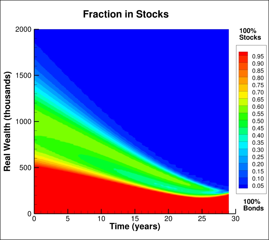
Figure 14.2 shows the optimal control heat maps for the fraction in stocks and withdrawal amounts, for the scenario in Table 10.1. Figure 2(a) shows a smooth behavior of the optimal fraction in stocks as a function of . This can be compared with the equivalent heat map for the EW-ES control in Forsyth 2022b (no tontine gains), which is much more aggressive at changing the asset allocation in response to changing wealth amounts. The smoothness of the controls in Figure 2(a) appears to be due to the rapid de-risking of a strategy which includes tontine gains, which provides a natural protection against sudden stock index drops. The upper blue zone in Figure 2(a) is de-risking due to the fact that, with sufficiently large wealth, there is essentially no probability of running out of cash even at the maximum withdrawal amount. The use of the stabilization factor forces the strategy to increase the weight in bonds for large values of wealth (see equation (6.2)).1313 13 “When you have won the game, stop playing,” William Bernstein. The lower red zone is in response to extremely poor wealth outcomes, which means that the optimal strategy is to invest 100% in stocks and hope for the best. However, this is an extremely unlikely outcome, as can be verified from Figure 1(b).
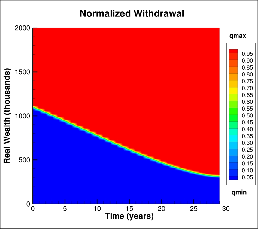
From Figure 2(b), we can observe that the optimal withdrawal strategy is essentially a bang-bang control, i.e. withdraw at either the maximum or minimum amount per year. This is not unexpected, as discussed in Appendix C. We also note that this type of strategy has been suggested previously, based on heuristic reasoning.1414 14 “If we have a good year, we take a trip to China,…if we have a bad year, we stay home and play canasta,” retired professor Peter Ponzo, discussing his DC plan withdrawal strategy https://www.theglobeandmail.com/report-on-business/math-prof-tests-investing-formulas-strategies/article22397218/ .
15 Discussion
Traditional annuities with true inflation protection are unavailable in Canada.1515 15 Some providers advertise annuities with inflation protection, however this is simply an escalating nominal payout, based on a fixed escalation rate. Since inflation is expected to be a major factor in the coming years, inflation protection is a valuable aspect of the optimal EW-ES strategy, with a tontine overlay.1616 16 Examination of historical periods of high inflation suggests that a portfolio of short term T-bills and an equal weight stock index generates significant positive real returns, see Forsyth 2022a. This strategy has an expected real withdrawal rate, over thirty years, of about 7% of the initial capital (per annum), never withdraws less than 4% of initial capital per annum, and a positive ES (expected shortfall) at the 5% level after thirty years.
Consequently, if we consider a retiree with no bequest motive, then joining a tontine pool, and following an optimal EW-ES strategy, is certainly an excellent alternative to a life annuity. Hence, it could be argued that, going forward, the EW-ES optimal tontine pool strategy has less risk than a conventional annuity.
Of course, there is no free lunch here. The reason that the tontine approach has a higher mean (and median) payout is that it is not guaranteed. There is some flexibility in the withdrawal amounts, and the portfolio contains risky assets. However, the ultimate risk, as measured by the expected shortfall at year thirty, is very small. We can also see that the median payout rises rapidly to the maximum withdrawal rate (8% real of the initial investment) within 3-4 years of retirement, and stays at the maximum for the remainder of the thirty year horizon.
As well, the investor forfeits the entire portfolio in the event of death. Although this is often considered a drawback, we remind the reader that annuities and defined benefit (DB) plans have this same property (restricting attention to a single retiree with no guarantee period).1717 17 Moshe Milevsky, an advocate of modern tontines, is quoted in the Toronto Star (April 13, 2021) as noting that “If you give up some of your money when you die, you can get more when you are alive.” Of course, it is possible to overlay various guarantees on to the tontine pool, e.g. a guarantee period, a money back guarantee, or joint and survivor benefits. The cost of these guarantees would, of course, reduce the expected annual withdrawals.
These results are robust to fees in the range of 50-100 bps per year. The long term results are also insensitive to random group gains.1818 18 The randomness of the group gain is due to fact that real tontine pools will be finite and heterogeneous.
However, the tontine gains (after fees) are comparatively small for retirees in the 65-70 age range. This suggests that it may be optimal to delay joining a tontine until the investor has attained an age of 70 or more.
Although we have explicitly excluded a bequest motive from our considerations, note that the median withdrawal strategy rapidly ramps up to the maximum withdrawal within a few years of retirement, and remains there for the entire remaining retirement period. Although it is commonly postulated that retirement consumption follows a U-shaped pattern, recent studies indicate that real retirement consumption falls with age (at least in countries which do not have large end of life expenses)(Brancati et al. 2015). In this case, the withdrawals which occur towards the end of the retirement period may exceed consumption. This allows the retiree to use these excess cash flows as a living bequest to relatives or charities.
16 Conclusions
DC plan decumulation strategies are typically based on some variant of the four per cent rule (Bengen 1994). However, bootstrap tests of these rules using historical data show a significant risk of running out of savings at the end of a thirty year retirement planning horizon.
This risk can be significantly reduced by using optimal stochastic control methods, where the controls are the asset allocation strategy and the withdrawal amounts (subject to maximum and minimum constraints)(Forsyth 2022b; Forsyth et al. 2020).
However, if we assume the retiree couples an optimal allocation/withdrawal strategy with participation in a tontine fund, then the risk of portfolio depletion after 30 years is virtually eliminated. At the same time, the cumulative total withdrawals are considerably increased compared with the previous two strategies. Of course, this comes at a price: the retiree forfeits her portfolio upon death. Hence the tontine overlay is most appealing to investors who have no bequest motivation, or who manage bequests using other funds.
We should also note that individual tontine accounts allow for complete flexibility in asset allocation strategies and do not require purchase of expensive investment products. These accounts are essentially peer-to-peer longevity risk management tools. Consequently, the custodian of these accounts bears no risk, and incurs only bookkeeping costs. Hence the fees charged by the custodian of these accounts can be very low. If desired, the retiree can pay for additional investment advice in a completely transparent manner.
17 Acknowledgements
Forsyth’s work was supported by the Natural Sciences and Engineering Research Council of Canada (NSERC) grant RGPIN-2017-03760. Vetzal’s work was supported by a Canadian Securities Institute Research Foundation grant 2021-2022.
18 Declaration
The authors have no conflicts of interest to report.
Appendix
Appendix A Induced Time Consistent Strategy
Denote the investor’s initial wealth at by . Then we have the following result:
Proposition A.1 (Pre-commitment strategy equivalence to a time consistent policy for an alternative objective function).
The pre-commitment EW-ES strategy determined by solving (with from equation ()) is the time consistent strategy for the equivalent problem (with fixed ), with value function defined by
| (A.1) | |||||
Proof.
This follows similar steps as in Forsyth 2020a, proof of Proposition 6.2, with the exception that the reward in Forsyth 2020a is expected terminal wealth, while here the reward is total withdrawals. ∎
Remark A.1 (An Implementable Strategy).
Given an initial level of wealth at , then the optimal control1919 19 To be perfectly precise here, in the event that the control is non-unique, we impose a tie-breaking strategy to generate a unique control. for the pre-commitment problem (6.2) is the same optimal control for the time consistent problem2020 20 Assuming that the same tie breaking strategy is used as for the pre-commitment problem. (A.1), . Hence we can regard problem as the EW-ES induced time consistent strategy. Thus, the induced strategy is implementable, in the sense that the investor has no incentive to deviate from the strategy computed at time zero, at later times (Forsyth 2020a).
Remark A.2 (EW-ES Induced Time Consistent Strategy).
In the following, we will consider the actual strategy followed by the investor for any as given by the induced time consistent strategy in equation (A.1), with a fixed value of , which is identical to the EW-ES strategy at time zero. Hence, we will refer to this strategy in the following as the EW-ES strategy, with the understanding that this refers to strategy for any .
Appendix B Numerical Techniques
We solve problems (6.2) using the techniques described in detail in Forsyth and Labahn 2019; Forsyth 2020a; Forsyth 2022b. We give only a brief overview here.
We localize the infinite domain to , and discretize using an equally spaced grid, with nodes. Similarly, we discretize on an equally spaced grid, with nodes. Localization errors are minimized using the domain extension method in (Forsyth and Labahn 2019).
At rebalancing dates, we solve the local optimization problem (7.7) by discretizing and using exhaustive search. Between rebalancing dates, we solve the two dimensional partial integro-differential equation (PIDE) (7.10 ) using Fourier methods (Forsyth and Labahn 2019; Forsyth 2022b). Finally, the optimization problem (7.4) is solved using a one-dimensional optimization technique.
We used the value in equation (7.2), which forces the investment strategy to be bond heavy if the remaining wealth in the investor’s account is large, and . Using this small value of gave the same results as for the summary statistics, to four digits. This is simply because the states with very large wealth have low probability. However, this stabilization procedure produced smoother heat maps for large wealth values, without altering the summary statistics appreciably.
B.1 Convergence Test: Synthetic Market
We compute and store the optimal controls from solving Problem 6.2 using the parametric model of the stock and bond processes. We then use the stored controls in Monte Carlo simulations to generate statistical results. As a robustness check, we also use the stored controls and simulate results using bootstrap resampling of historical data.
Table B.1 shows a detailed convergence test for the base case problem given in Table 10.1, for the EW-ES problem. The results are given for a sequence of grid sizes, for the dynamic programming algorithm in Section 7 and Appendix B. The dynamic programming algorithm appears to converge at roughly a second order rate. The optimal control computed using dynamic programming is stored, and then used in Monte Carlo computations. The MC results are in good agreement with the dynamic programming solution.
For all the numerical examples, we will use the grid, since this seems to be accurate enough for our purposes.
| Algorithm in Section 7 and Appendix B | Monte Carlo | ||||
|---|---|---|---|---|---|
| Grid | ES (5%) | Value Function | ES (5%) | ||
| 108.13 | 67.99 | 2059.60 | 123.26 | 68.04 | |
| 158.88 | 67.79 | 2063.19 | 164.45 | 67.81 | |
| 201.88 | 67.56 | 2064.27 | 203.87 | 67.56 | |
| 206.56 | 67.54 | 2064.54 | 207.70 | 67.54 | |
| Algorithm in Section 7 and Appendix B | Monte Carlo | ||||
|---|---|---|---|---|---|
| Grid | ES (5%) | Value Function | ES (5%) | ||
| -203.31 | 54.08 | 860.033 | -191.99 | 53.96 | |
| -191.40 | 53.58 | 889.613 | -188.07 | 53.53 | |
| -188.91 | 53.57 | 898.712 | -188.14 | 53.55 | |
| -188.04 | 53.54 | 901.106 | -187.95 | 53.53 | |
Appendix C Continuous Withdrawal/Rebalancing Limit
In order to develop some intuition about the nature of the optimal controls, we will examine the limit as the rebalancing interval becomes vanishingly small.
Proposition C.1 (Bang-bang withdrawal control in the continuous withdrawal limit).
Assume that
- •
- •
the portfolio is continuously rebalanced, and withdrawals occur at a continuous (finite) rate ,
- •
the HJB equation for the EW-ES problem in the continuous rebalancing limit has bounded derivatives w.r.t. total wealth,
- •
in the event of ties for the control , the smallest withdrawal is selected,
then the optimal withdrawal control for the EW-ES problem and for the EW-LS problem is bang-bang, .
Proof.
This follows the same steps as in Forsyth 2022b. ∎
Remark C.1 (Bang-bang control for discrete rebalancing/withdrawals).
Proposition C.1 suggests that, for sufficiently small rebalancing intervals, we can expect the optimal control (finite withdrawal amount) to be bang-bang, i.e. it is only optimal to withdraw either the maximum amount or the minimum amount . However, it is not clear that this will continue to be true for the case of yearly rebalancing (which we specify in our numerical examples), and finite amount controls . In fact, we do observe that the finite amount control is very close to bang-bang in our numerical experiments, even for yearly rebalancing.
Appendix D Detailed Efficient Frontiers: Synthetic Market
| ES (5%) | ||||
|---|---|---|---|---|
| 0.15 | 70.06 | -309.569 | 189.48 | .490 |
| 0.170 | 70.04 | -270.13 | 185.19 | .489 |
| .180 | 68.51 | 46.77 | 599.42 | 385.28 |
| .185 | 67.56 | 203.87 | 820.65 | 585.97 |
| .20 | 66.41 | 384.76 | 1058.40 | 802.40 |
| 0.25 | 63.85 | 732.34 | 1517.04 | 1220.33 |
| 0.30 | 62.22 | 912.29 | 1754.40 | 1439.83 |
| 0.50 | 58.48 | 1209.40 | 2120.59 | 1802.19 |
| 1.0 | 54.81 | 1372.46 | 2327.42 | 2021.22 |
| 10.0 | 48.96 | 1457.52 | 2484.58 | 2151.79 |
| 40 | 1460.76 | 2885.85 | 2173.04 |
| ES (5%) | ||||
|---|---|---|---|---|
| 0.180 | 69.17 | -823.76 | -2.51 | -691.81 |
| 1.0 | 61.38 | -319.66 | -39.47 | -229.18 |
| 1.5 | 58.98 | -260.92 | -65.88 | -179.60 |
| 1.75 | 57.97 | -242.34 | -74.74 | -161.25 |
| 2.5 | 55.86 | -211.03 | -81.44 | -132.87 |
| 3.75 | 53.55 | -188.14 | -81.11 | -107.00 |
| 5.0 | 52.08 | -177.88 | -78.39 | -90.10 |
| 6.25 | 51.29 | -173.59 | -79.08 | -89.03 |
| 7.5 | 50.72 | -171.05 | -79.3 | -88.25 |
| 10.0 | 49.89 | -168.16 | -78.77 | -87.18 |
| 100.0 | 46.41 | -162.86 | -68.28 | -77.47 |
| 40.0 | -162.67 | +5.72 | -76.0 |
Appendix E Detailed Efficient Frontiers: Historical Market
| ES (5%) | |||
|---|---|---|---|
| 0.15 | 71.25 | -165.23 | 157.16 |
| .170 | 71.01 | -138.15 | 153.13 |
| .180 | 68.94 | 204.20 | 573.29 |
| .185 | 67.99 | 369.26 | 769.96 |
| .20 | 66.64 | 546.98 | 1038.07 |
| .25 | 63.84 | 863.20 | 1500.51 |
| 0.30 | 62.08 | 1011.55 | 1739.21 |
| 0.5 | 58.13 | 1211.18 | 2115.22 |
| 1.0 | 54.50 | 1285.93 | 2330.33 |
| 10.0 | 49.42 | 1275.98 | 2485.58 |
| 40 | 1280.97 | 2892.41 |
| ES (5%) | |||
|---|---|---|---|
| .180 | 69.91 | -805.65 | -31.84 |
| 1.0 | 61.77 | -290.03 | -40.87 |
| 1.5 | 59.21 | -248.15 | -77.26 |
| 1.75 | 58.16 | -235.46 | -78.50 |
| 2.5 | 6.02 | -219.00 | -81.84 |
| 3.75 | 53.78 | -209.9 | -80.68 |
| 5.0 | 52.43 | -207.15 | -77.25 |
| 6.25 | 51.74 | -209.02 | -78.11 |
| 7.5 | 51.26 | -210.38 | -78.48 |
| 10.0 | 50.58 | -212.41 | -77.95 |
| 100.0 | 47.72 | -217.82 | -67.91 |
| 40.0 | -219.16 | +17.34 |
References
- Anarkulova et al. (2022) Anarkulova, A., S. Cederburg, and M. S. O’Doherty (2022). Stocks for the long run? Evidence from a broad sample of developed markets. Journal of Financial Economics 143:1, 409–433.
- Bar and Gatzert (2022) Bar, M. and N. Gatzert (2022). Products and strategies for decumulation of wealth during retirement: insights from the literature. North American Actuarial Journal. DOI: 10.1080/10920277.2022.2078374.
- Bengen (1994) Bengen, W. (1994). Determining withdrawal rates using historical data. Journal of Financial Planning 7, 171–180.
- Brancati et al. (2015) Brancati, C., B. Beach, and B. Frankin (2015). Understanding retirement journeys: Expectations vs reality. International Longevity Centre UK, https://www.bl.uk/collection-items/understanding-retirement-journeys-expectations-vs-reality.
- Braughtigam et al. (2017) Braughtigam, M., M. Guillen, and J. P. Nielsen (2017). Facing up to longevity with old actuarial methods: a comparison of pooled funds and income tontines. Geneva papers on risk and insurance 42, 406–422.
- Cavaglia et al. (2022) Cavaglia, S., L. Scott, K. Blay, and S. Hixon (2022). Multi-asset class factor premia: A strategic asset allocation perspective. The Journal of Portfolio Management 48:9, 14–32.
- Chen et al. (2021) Chen, A., M. Guillen, and M. Rach (2021). Tontine fees. Insurance: Mathematics and Economics 100, 89–106.
- Chen et al. (2021) Chen, A., P. Hieber, and M. Rach (2021). Optimal retirement products under subjective mortality beliefs. Insurance: Mathematics and Economics 101:A, 55–69.
- Chen and Rach (2022) Chen, A. and M. Rach (2022). The tontine puzzle. SSRN 4106903.
- Cogneau and Zakalmouline (2013) Cogneau, P. and V. Zakalmouline (2013). Block bootstrap methods and the choice of stocks for the long run. Quantitative Finance 13, 1443–1457.
- Cont and Mancini (2011) Cont, R. and C. Mancini (2011). Nonparametric tests for pathwise properties of semimartingales. Bernoulli 17, 781–813.
- Dang and Forsyth (2016) Dang, D.-M. and P. A. Forsyth (2016). Better than pre-commitment mean-variance portfolio allocation strategies: a semi-self-financing Hamilton-Jacobi-Bellman equation approach. European Journal of Operational Research 250, 827–841.
- Denuit and Vernic (2018) Denuit, M. and R. Vernic (2018). Bivariate Bernoulli weighted sums and distribution of single period Tontine benefits. Methodology and Computing in Applied Probability 20, 1403–1416.
- Dichtl et al. (2016) Dichtl, H., W. Drobetz, and M. Wambach (2016). Testing rebalancing strategies for stock-bond portfolos across different asset allocations. Applied Economics 48, 772–788.
- Donnelly (2015) Donnelly, C. (2015). Actuarial fairness and solidarity in pooled annuity funds. ASTIN Bulletin 45, 49–74.
- Donnelly et al. (2014) Donnelly, C., M. Guillen, and J. B. Nielsen (2014). Bringing cost transparency to the life annuity market. Insurance: Mathematica and Economics 56, 14–27.
- Forsyth and Labahn (2019) Forsyth, P. and G. Labahn (2019). Monotone Fourier methods for optimal stochastic control in finance. Journal of Computational Finance 22:4, 25–71.
- Forsyth (2020a) Forsyth, P. A. (2020a). Multi-period mean CVAR asset allocation: Is it advantageous to be time consistent? SIAM Journal on Financial Mathematics 11:2, 358–384.
- Forsyth (2020b) Forsyth, P. A. (2020b). Optimal dynamic asset allocation for DC plan accumulation/decumulation: Ambition-CVAR. Insurance: Mathematics and Economics 93, 230–245.
- Forsyth (2022a) Forsyth, P. A. (2022a). Asset allocation during high inflation periods: A stress test. https://cs.uwaterloo.ca/˜paforsyt/inflation_stress_test.pdf.
- Forsyth (2022b) Forsyth, P. A. (2022b). A stochastic control approach to defined contribution plan decumulation: “The Nastiest, Hardest Problem in Finance”. North American Actuarial Journal 26:2, 227–252.
- Forsyth and Vetzal (2019) Forsyth, P. A. and K. R. Vetzal (2019). Optimal asset allocation for retirement savings: deterministic vs. time consistent adaptive strategies. Applied Mathematical Finance 26:1, 1–37.
- Forsyth et al. (2020) Forsyth, P. A., K. R. Vetzal, and G. Westmacott (2020). Optimal asset allocation for a DC pension decumulation with a variable spending rule. ASTIN Bulletin 50:2, 419–447.
- Fuentes et al. (2022) Fuentes, O. M., R. K. Fullmer, and M. Garcia-Huitron (2022). A sustainable, variable lifetime retirement income solution for the Chilean pension system. SSRN 4045646 https://ssrn.com/abstract=4045646.
- Fullmer (2019) Fullmer, R. K. (2019). Tontines: a pracitioner’s guide to mortality-pooled investments. CFA Institute Research Foundation https://www.cfainstitute.org/en/research/foundation/2019/tontines.
- Fullmer and Forman (2022) Fullmer, R. K. and J. B. Forman (2022). State sponsored pensions for private sector workers. In O. S. Mitchell (Ed.), New models for managing longevity risk, Chapter 10, pp. 171–206. Oxford: Oxford University Press.
- Fullmer and Sabin (2019) Fullmer, R. K. and M. J. Sabin (2019). Individual tontine accounts. Journal of Accounting and Finance 19:8, 31–61.
- Guyton and Klinger (2006) Guyton, J. T. and W. J. Klinger (2006). Decision rules and maximum initial withdrawal rates. Journal of Financial Planning 19(3), 48–58.
- Hatch and White (1985) Hatch, J. E. and R. W. White (1985). Canadian stocks, bonds, bills and inflation: 1950-1983. Financial Analysts Research Foundation Mongraph Series, Number 19.
- Irlam (2014) Irlam, G. (2014). Portfolio size matters. Journal of Personal Finance 13(2), 9–16.
- Kou (2002) Kou, S. G. (2002). A jump-diffusion model for option pricing. Management Science 48, 1086–1101.
- Kou and Wang (2004) Kou, S. G. and H. Wang (2004). Option pricing under a double exponential jump diffusion model. Management Science 50, 1178–1192.
- Li and Forsyth (2019) Li, Y. and P. A. Forsyth (2019). A data driven neural network approach to optimal asset allocation for target based defined contribution pension plans. Insurance: Mathematics and Economics 86, 189–204.
- Lin et al. (2015) Lin, Y., R. MacMinn, and R. Tian (2015). De-risking defined benefit plans. Insurance: Mathematics and Economics 63, 52–65.
- MacDonald et al. (2013) MacDonald, B.-J., B. Jones, R. J. Morrison, R. L. Brown, and M. Hardy (2013). Research and reality: A literature review on drawing down retirement financial savings. North American Actuarial Journal 17, 181–215.
- MacDonald et al. (2021) MacDonald, B. J., B. Sanders, L. Strachan, and M. Frazer (2021). Affordable Lifetime Pension Income for a Better Tomorrow. How we can address the 1.5 trillion decumulation disconnect in the Canadian retirement income system with Dynamic Pension pools. National Institute on Ageing, Ryerson University and Global Risk Institute, https://globalriskinstitute.org/publications/affordable-lifetime-pension-income-for-a-better-tomorrowhow-we-can-address-the-1-5-trillion-decumulation-disconnect-in-the-canadian-retirement-income-system-with-dynamic-pension-pools/.
- MacMinn et al. (2014) MacMinn, R., P. Brockett, J. Wang, Y. Lin, and R. Tian (2014). The securitization of longevity risk and its implications for retirement security. In O. S. Mitchell, R. Maurer, and P. B. Hammond (Eds.), Recreating Sustainable Retirement, pp. 134–160. Oxford: Oxford University Press.
- Mancini (2009) Mancini, C. (2009). Non-parametric threshold estimation models with stochastic diffusion coefficient and jumps. Scandinavian Journal of Statistics 36, 270–296.
- Milevsky (2022) Milevsky, M. (2022). How to build a modern tontine. Toronto: Springer.
- Milevsky and Salisbury (2015) Milevsky, M. A. and T. S. Salisbury (2015). Optimal retirement income tontines. Insurance: Mathematics and Economics 64, 91–105.
- Ni et al. (2022) Ni, C., Y. Li, P. A. Forsyth, and R. Caroll (2022). Optimal asset allocation for outperforming a stochastic benchmark. Quantitative Finance 22(9), 1595–1626.
- OECD (2019) OECD (2019). Pension markets in focus. https://www.oecd.org/daf/fin/private-pensions/Pension-Markets-in-Focus-2019.pdf.
- Patton et al. (2009) Patton, A., D. Politis, and H. White (2009). Correction to: automatic block-length selection for the dependent bootstrap. Econometric Reviews 28, 372–375.
- Peijnenburg et al. (2016) Peijnenburg, K., T. Nijman, and B. J. Werker (2016). The annuity puzzle remains a puzzle. Journal of Economic Dynamics and Control 70, 18–35.
- Politis and Romano (1994) Politis, D. and J. Romano (1994). The stationary bootstrap. Journal of the American Statistical Association 89, 1303–1313.
- Politis and White (2004) Politis, D. and H. White (2004). Automatic block-length selection for the dependent bootstrap. Econometric Reviews 23, 53–70.
- Rockafellar and Uryasev (2000) Rockafellar, R. T. and S. Uryasev (2000). Optimization of conditional value-at-risk. Journal of Risk 2, 21–42.
- Sabin and Forman (2016) Sabin, M. J. and J. B. Forman (2016). The analytics of a single period tontine. SSRN 2874160.
- Shefrin and Thaler (1988) Shefrin, H. M. and R. H. Thaler (1988). The behavioral life-cycle hypothesis. Economic Inquiry 26, 609–643.
- Simonian and Martirosyan (2022) Simonian, J. and A. Martirosyan (2022). Sharpe parity redux. The Journal of Portfolio Management 48:9, 183–193.
- Strub et al. (2019) Strub, M., D. Li, and X. Cui (2019). An enhanced mean-variance framework for robo-advising applications. SSRN 3302111.
- Thaler (1990) Thaler, R. H. (1990). Anomalies: Savings, fungibility, and mental accounts. Journal of Economic Perspectives 4(1), 193–205.
- van Benthem et al. (2018) van Benthem, L., L. Frehen, J. Cramwinckel, and R. de Kort (2018). Tonchain: the future of pensions? VBA Journal 134:Summer, 18–22.
- van Staden et al. (2018) van Staden, P. M., D.-M. Dang, and P. Forsyth (2018). Time-consistent mean-variance portfolio optimization: a numerical impulse control approach. Insurance: Mathematics and Economics 83, 9–28.
- Waring and Siegel (2015) Waring, M. B. and L. B. Siegel (2015). The only spending rule article you will ever need. Financial Analysts Journal 71(1), 91–107.
- Weinert and Grundi (2021) Weinert, J.-H. and H. Grundi (2021). An innovative instrument for longevity risk management in an aging society. European Actuarial Journal 11, 49–86.
- Winter and Planchet (2022) Winter, P. and F. Planchet (2022). Modern tontines as a pension solution: a practical overview. European Actuarial Journal 12, 3–32.