Hydraulic Parameter Estimation in District Heating Networks

The type of network under consideration consists of two directed sub-graphs, a supply-network $\bar{\mathcal{G}}=(\bar{\mathcal{E}},\bar{\mathcal{N}})$ and a return-network $\underaccent{\bar}{\mathcal{G}}=(\underaccent{\bar}{\mathcal{E}},\underaccent{\bar}{\mathcal{N}})$. They are symmetric in structure. In addition, there is a set of boundary edges $\mathring{\mathcal{E}}$ that are connected from some nodes in $\bar{\mathcal{N}}$ to their equivalent counterparts in $\underaccent{\bar}{\mathcal{N}}$. Define also two reference nodes $\alpha\in\bar{\mathcal{N}}$ and $\beta\in\underaccent{\bar}{\mathcal{N}}$, and assume all edges in $\bar{\mathcal{E}}$ and $\underaccent{\bar}{\mathcal{E}}$ to be directed away from $\alpha$ and $\beta$ respectively. Non-reference nodes which are not connected to a boundary edge are called internal nodes, and are assumed to have at least degree three. Denote a path $\mathcal{P}$ to be a set of ordered edges traversing a set of ordered, distinct nodes.

Figure 1 illustrates such a network. Here $\bar{\mathcal{N}}=(\alpha,1,2,3,4,5)$, $\underaccent{\bar}{\mathcal{N}}=(\beta,6,7,8,9,10)$, $\bar{\mathcal{E}}=(1,2,3,4,5)$ $\underaccent{\bar}{\mathcal{E}}=(9,10,11,12,13)$ and $\mathring{\mathcal{E}}=(6,7,8)$. Internal nodes are $4$, $5$, $9$ and $10$. The highlighted path $\mathcal{P}=(1,3,4,7,12,11,9)$ traverses the nodes $(\alpha,4,5,2,7,10,9,\beta)$.

Associate each edge $e$ with a volumetric flow rate $q_{e}$. Denote the vectors of such flows $\bar{q}$, $\underaccent{\bar}{q}$ and $\mathring{q}$ for supply, return and boundary edges respectively. Associate with each node $n$ a pressure-value $p_{n}$. Denote the vectors of such pressures $\bar{p}$ and $\underaccent{\bar}{p}$ for supply and return nodes respectively. Associate with each edge $e$ a control value $u_{e}\in\left]0,1\right]$, and let $u_{e}=1$ for $e\in\bar{\mathcal{E}}\cup\underaccent{\bar}{\mathcal{E}}$. An edge $e$ also has an unknown resistance parameter $s_{e}$, which is the parameter we seek to estimate in this paper. Denote $\bar{s}$, $\underaccent{\bar}{s}$ and $\mathring{s}$ to be the vectors of such parameters related to edges in $\bar{\mathcal{E}}$, $\underaccent{\bar}{\mathcal{E}}$ and $\mathring{\mathcal{E}}$ respectively. Assume symmetry between characteristics of supply and return edges such that $\bar{s}=\underaccent{\bar}{s}$.

Each node is subject to preservation of mass, i.e. the sum of incoming flow must equal the sum of outgoing flow. Considering first the supply-network, this can be equivalently written as

$$\begin{bmatrix}\mathring{q}\\ 0\end{bmatrix}=\bar{B}\bar{q}$$

(1)

where $\bar{B}=\left[\bar{B}_{i,j}\right]$ is the basic incidence matrix of $\bar{\mathcal{G}}$, defined as

$$\bar{B}_{i,j}=\begin{cases}1,&\text{if edge j leads to node i}\\ -1,&\text{if edge j leads away from node i}\\ 0,&\text{if edge j is not connected to node i.}\end{cases}$$

(2)

Here the node $\alpha$ is omitted to ensure (1) is not over-determined. Note that in (1), it is assumed without loss of generality that the nodes are ordered such that internal nodes come last. See e.g. the network visible in Figure 1 for which

$$\bar{B}=\begin{bmatrix}0&1&0&0&0\\ 0&0&0&1&0\\ 0&0&0&0&1\\ 1&-1&-1&0&0\\ 0&0&1&-1&-1\\ \end{bmatrix}.$$

(3)

Due to the tree-structure of $\bar{\mathcal{G}}$, $\bar{B}$ is invertible. This means that given known boundary flows $\mathring{q}$, the supply-flows $\bar{q}$ can be calculated as

$$\bar{q}=\bar{B}^{-1}\begin{bmatrix}\mathring{q}\\ 0\end{bmatrix}.$$

(4)

Due to symmetry between $\bar{\mathcal{G}}$ and $\underaccent{\bar}{\mathcal{G}}$, the corresponding basic incidence matrix $\underaccent{\bar}{B}=\bar{B}$. This in combination with the boundary flows $\mathring{q}$ being directed from $\bar{\mathcal{G}}$ to $\underaccent{\bar}{\mathcal{G}}$ gives

$$\underaccent{\bar}{q}=-\bar{q}.$$

(5)

For an edge $e$ with flow $q_{e}$, directed from node $n$ to node $m$ with pressures $p_{n}$ and $p_{m}$, models of the following type are considered.

$$p_{n}-p_{m}=f(q_{e},u_{e})s_{e},$$

(6)

where $s_{e}$ is the unknown resistance parameter to estimate and $f:\mathbb{R}\times\left]0,1\right]\rightarrow{}\mathbb{R}$ is a given continuous function satisfying

		$\displaystyle f(q,u)=-f(-q,u),$		(7)
		$\displaystyle f(0,u)=0,$		(8)
		$\displaystyle q_{i}>q_{j}\implies f(q_{i},u)>f(q_{j},u),$		(9)
		$\displaystyle u_{i}>u_{j}\implies f(q,u_{i})<f(q,u_{j}),$		(10)
		$\displaystyle q>0\implies\lim_{u\to 0}f(q,u)=\infty.$		(11)

A specific choice of $f$ will be presented in section 5, where a numerical example is investigated.

Consider all paths $\mathcal{P}_{v}$ that lead from $\alpha$ to $\beta$ via a boundary edge $v\in\mathring{\mathcal{E}}$. Denote $n_{b}$ to be the number of such paths, i.e. the number of boundary edges. The path $\mathcal{P}$ in Figure 1 is an example of such a path. Then

$$p_{\alpha}-p_{\beta}=\sum_{e\in\mathcal{P}_{v}\cap\bar{\mathcal{E}}}f(q_{e},1)s_{e}-\sum_{e\in\mathcal{P}_{v}\cap\underaccent{\bar}{\mathcal{E}}}f(q_{e},1)s_{e}+f(q_{v},u_{v})s_{v}$$

(12)

for all $v$. This equation is the result of subsequent uses of (6). Note that $e\notin\mathring{\mathcal{E}}\implies u_{e}=1$. The signs in front of the sums are decided by the direction of edges in the supply (return) network being directed from $\alpha$ ($\beta$).

Since $\bar{\mathcal{G}}$ and $\underaccent{\bar}{\mathcal{G}}$ are symmetrical, the sets $\mathcal{P}_{v}\cap\bar{\mathcal{E}}$ and $\mathcal{P}_{v}\cap\underaccent{\bar}{\mathcal{E}}$ contain the symmetrically corresponding edges. Using (5), (7) and the assumption $\bar{s}=\underaccent{\bar}{s}$,

$$p_{\alpha}-p_{\beta}=\sum_{e\in\mathcal{P}_{v}\cap\bar{\mathcal{E}}}2f(q_{e},1)s_{e}+f(q_{v},u_{v})s_{v}.$$

(13)

Considering (13) for all $n_{b}$ paths at once yields

$$Fs=\mathbf{1}(p_{\alpha}-p_{\beta}).$$

(14)

Here $s=\left[\bar{s}^{T},\mathring{s}^{T}\right]^{T}$ is a vector of $n_{s}$ resistances and $F=\left[F_{i,j}\right]$ is an $n_{b}\times n_{s}$ matrix defined as

$$F_{i,j}=\begin{cases}2f(q_{j},1),&\text{if }j\in\mathcal{P}_{i}\cap\bar{\mathcal{E}}\\ f(q_{j},u_{j}),&\text{if }j\in\mathcal{P}_{i}\cap\mathring{\mathcal{E}}\\ 0,&\text{else.}\end{cases}$$

(15)

For parameter estimation, we will use several samples of steady state measurements. Denote any such steady state of pressures, flows and valve positions in the network a load condition $t$. For example $\mathring{q}(t)$ is the vector of boundary flows $\mathring{q}$ at load condition $t$. The parameter estimation problem is therefore:

Let $F(t)$ be defined by (14) for one load condition $t$. Note that $F(t)$ can be constructed using only the boundary flows $\mathring{q}(t)$ and the controller settings $u(t)$. Using the measurements defined in Problem 1, the equation

$$\begin{bmatrix}F(1)\\ F(2)\\ \vdots\\ F(T)\end{bmatrix}s=\begin{bmatrix}\mathbf{1}(p_{\alpha}(1)-p_{\beta}(1))\\ \mathbf{1}(p_{\alpha}(2)-p_{\beta}(2))\\ \vdots\\ \mathbf{1}(p_{\alpha}(T)-p_{\beta}(T))\end{bmatrix}$$

(16)

can be constructed. Let $\Phi$ be the matrix in the left hand side of (16) and $y$ be the right hand side of (16) such that (16) can be condensed to

$$\Phi s=y.$$

(17)

Note that linear constraints were constructed also in [9] and [10]. Our extension is twofold: They required the measurement of pressure at each boundary node, while we use only $p_{\alpha}$ and $p_{\beta}$. In addition we include modeling of the valve characteristics which is important for control applications.

If (17) has a unique solution, a solution $\hat{s}$ to problem 1 can be obtained as

$$\hat{s}=\Phi^{\dagger}y,$$

(18)

where $\dagger$ denotes the the Moore-Penrose pseudoinverse. In a real application, $\Phi$ and $y$ will be subject to measurement noise as well as errors in the model assumption, and in this case (18) chooses the $\hat{s}$ of minimum Euclidean norm which minimizes the Euclidean distance between observed and estimated values for $y$. While (18) is the method used in this paper, the linear constraints of (17) can be used in other optimization frameworks. For instance, parameter positivity constraints, other cost functions or other parameter regularization methods could be considered.

Theorem 1 is stated in terms of each load condition $t$ used in constructing $\Phi$. However, if (19) does not hold in general, i.e. for any set of load conditions that could feasibly be sampled, it becomes unlikely to hold for all $t$ if $T$ is large. Thus Given general $q_{e}$, $q_{v}$, $\theta_{v}$, we investigate if

$$\sum_{e\in\mathcal{P}_{v}\cap\bar{\mathcal{E}}}2f(q_{e},1)\lambda_{e}+f(q_{v},u_{v})\lambda_{v}=0$$

(21)

holds for any $\lambda\neq 0$. If not, we can conclude that it’s unlikely that (19) holds for all $t$ unless load conditions were sampled with some form of bias.

Assume that there is a $\lambda\neq 0$ such that (21) holds. In addition, assume there is a $v$ such that $\lambda_{v}\neq 0$. That would imply that

$$f(q_{v},u_{v})=-\frac{\sum_{e\in\mathcal{P}_{v}\cap\bar{\mathcal{E}}}2f(q_{e},1)\lambda_{e}}{\lambda_{v}},$$

(22)

i.e. there is a function mapping flows $q_{e}$ in edges in $\mathcal{P}_{v}$ to $f(q_{v},u_{v})$. As a contradiction, consider the following proposition.

Proposition 1 shows that $f(q_{v},u_{v})$ is decided by (24), $f(q_{v},u_{v})$ is a sum of $p_{\alpha}-p_{\beta}$ and a function of the flows along the edges of the path. Since Proposition 1 states that any boundary flow vector $\mathring{q}>0$ and sufficiently large $p_{\alpha}-p_{\beta}$ is feasible, $f(q_{v},u_{v})$ is clearly not only a function of the flows, but also $p_{\alpha}-p_{\beta}$. This contradicts (22). Thus if there is a $\lambda$ that fulfills (21), then $\lambda_{v}=0$.

If $\lambda_{v}=0$ as previously shown, then returning to (21) and analyzing one edge $i\in\mathcal{P}_{v}$ yields

$$f(q_{i},1)=\frac{\sum_{e\in\mathcal{P}_{v}\cap\bar{\mathcal{E}},e\neq i}2f(q_{e},1)\lambda_{e}}{\lambda_{i}}.$$

(25)

I.e. there is a function of the other flows $q_{e}$ in $\mathcal{P}_{v}$ yielding $f(q_{i},1)$. (9) gives that $f$ is monotone in $q_{i}$. This means that (25) implies that $q_{i}$ can be decided as a function of the other flows $q_{e}$ in the path. To contradict this, consider the following proposition.

If (25) would hold, it implies that $q_{i}$ as analyzed in Proposition 2 is a function of the other flows along the path. However, as Proposition 2 states, there is no such function but rather $q_{i}$ can take any value within a range. The only conclusion is thus that $\lambda_{e}=0$ for all $e$.

Section 4.2 shows that there is no $\lambda$ where $\lambda_{v}\neq 0$ for any $v\in\mathring{\mathcal{E}}$ such that (21) holds in general. This section showed that there is no $\lambda_{e}\neq 0$ for any $e\in\bar{\mathcal{E}}$ such that (21) holds in general. This leads to the conclusion that the only solution to (21) is $\lambda=0$. If load conditions are not sampled with some bias, it is therefore likely that the conditions of Theorem 1 should hold, especially if the number of load conditions $T$ is large.

We consider a district heating model example where all edges $e$ in the supply-and-return networks are pipes. They are described by pressure-relations

$$f(q_{e},1)\cdot s_{e}=q_{e}|q_{e}|\cdot\frac{2f_{d,e}\rho L}{\pi^{2}D_{e}^{5}},$$

(30)

where $f_{d,e}$ is the Darcy friction factor, $\rho$ is the density of the water, $L$ is the length of the pipe and $D_{e}$ is the diameter of the pipe, all assumed to be constant in time and and along the length of the pipe.

All boundary edges are control valves in customer substations, regulating the flow of hot water these customers receive. Control valves $v$ have different characteristics in their mapping from valve position $u_{v}$ to flow rate $q_{v}$ at a given differential pressure. In district heating substations, this characteristic is often linear as stated in [1]. We express this as

$$f(q_{v},u_{v})\cdot s_{v}=\frac{q_{v}|q_{v}|}{u_{v}^{2}}\cdot\frac{1}{k_{v}^{2}}$$

(31)

for valve $v$ with valve setting $u_{v}$, where $k_{v}$ is a linear parameter for the relation between flow and valve position.

The example network under consideration is shown in Figure 2. This is the same network topology as was considered in [10], but now with added boundary edges and return network. Edges 1-6 are valves and edges 7-28 are pipes.

The load conditions $t=1\dots T$ used in the numerical examples are generated the following way:

1. 1.

   A set of boundary-flows $\mathring{q}(t)$ are sampled uniformly in the range $\left[100,200\right]$.

2. 2.

   Supply-network flows $\bar{q}(t)$ are calculated through (4).

3. 3.

   The pressure drop in each supply-network edge is calculated using (30).

4. 4.

   $p_{\alpha}-p_{\beta}$ is randomly selected sufficiently large such that (23) is feasible for all valves $v$.

5. 5.

   The corresponding feasible valve positions $u_{v}$ are calculated from (24).

Noisy measurements are considered. If $x$ is a value generated by the above procedure, then the value used in the estimation process will be $\hat{x}$, sampled uniformly in the range $\left[x(1-\epsilon),x(1+\epsilon)\right]$ where $\epsilon$ denotes the noise level.

The deterministic case $\epsilon=0$ is considered first, followed by the noisy case $\epsilon=0.01$.

First we estimate the parameters using noise-free measurements under four load conditions. Table 1 presents the actual and estimated hydraulic parameters. Note that the pipe pairs 9-20 and 15-26 differ in parameters between supply and return, contrary to the assumptions of this paper. All parameters are estimated accurately except for these pairs. Note however, that $\hat{s}_{9}+\hat{s}_{20}=s_{9}+s_{20}$ and $\hat{s}_{15}+\hat{s}_{26}=s_{15}+s_{26}$. This is logical since this sum is utilized in reducing (12) to (13), which defines $\Phi$. If as in [9] and [10] more pressure-measurements are available, individual parameters should be possible to estimate. However for many control applications such as [6], only the sum is required.

Table 1 shows also the result of estimation when using $\epsilon=0.01$ (a maximum 1 % measurement error) and 100 load conditions. The parameters are still determined accurately.

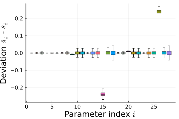
Figures 3(a) and 3(b) show the confidence interval of the parameter estimates for edges $5$ and $11$ using increasing numbers of load conditions. For each point on the graphs, 1000 estimations are performed. These plots show that both for boundary edges and supply-side edges, the accuracy increases with the number of load conditions. In addition Figure 3(c) shows the boxplot of estimates using 50 load conditions, showing that all parameters are decided with reasonable accuracy, save for the previously discussed pairs 9-20 and 15-26 where instead the sum is accurate.

The function $f$ in this numerical example does not fit all possible component characteristics. For instance, [9] consider equal percentage valves, rather than linear valves. In such a case, one can consider a kernel of functions $f_{1},f_{2},\dots,f_{n}$, such that the pressure difference over each edge can be described as

$p_{n}-p_{m}\approx f_{1}(q_{e},u_{e})s_{e,1}+f_{2}(q_{e},u_{e})s_{e,2}+\dots+f_{n}(q_{e},u_{e})s_{e,n}.$

(32)

More component types can be parameterized and considered. For instance, some boundary nodes could be by pumps, representing other producers in the network. Some of the edges in supply/return-networks could be booster pumps or valves.

Lastly, a generalization to meshed networks would be highly desirable. This is however difficult, as the linearity of the constraints (17) are based on calculating all edge flows explicitly.

References

- [1] S. Frederiksen and S. Werner, District heating and cooling. Studentlitteratur, 2013.
- [2] H. Lund, P. A. Østergaard, M. Chang, S. Werner, S. Svendsen, P. Sorknæs, J. E. Thorsen, F. Hvelplund, B. O. G. Mortensen, B. V. Mathiesen, C. Bojesen, N. Duic, X. Zhang, and B. Möller, “The status of 4th generation district heating: Research and results,” Energy, vol. 164, pp. 147–159, 2018.
- [3] A. Vandermeulen, B. van der Heijde, and L. Helsen, “Controlling district heating and cooling networks to unlock flexibility: A review,” Energy, vol. 151, pp. 103–115, May 2018.
- [4] L. Brange, K. Sernhed, and M. Thern, “Decision-making process for addressing bottleneck problems in district heating networks,” International Journal of Sustainable Energy Planning and Management, vol. 20, pp. 37–50, 2019.
- [5] Y. Wang, S. You, H. Zhang, W. Zheng, X. Zheng, and Q. Miao, “Hydraulic performance optimization of meshed district heating network with multiple heat sources,” Energy, vol. 126, pp. 603–621, 03 2017.
- [6] F. Agner, P. Kergus, R. Pates, and A. Rantzer, “Combating district heating bottlenecks using load control,” Smart Energy, vol. 6, p. 100067, 2022.
- [7] D. A. Savic, Z. S. Kapelan, and P. M. Jonkergouw, “Quo vadis water distribution model calibration?,” Urban Water Journal, vol. 6, no. 1, pp. 3–22, 2009.
- [8] G. Yin, B. Wang, T. Sheng, H. Sun, Q. Guo, and Z. Qiao, “Network parameter estimation for district heating system,” in 2018 2nd IEEE Conference on Energy Internet and Energy System Integration (EI2), pp. 1–6, 2018.
- [9] N. Wang, S. You, Y. Wang, H. Zhang, Q. Miao, X. Zheng, and L. Mi, “Hydraulic resistance identification and optimal pressure control of district heating network,” Energy and Buildings, vol. 170, pp. 83–94, 2018.
- [10] Y. Liu, P. Wang, and P. Luo, “Pipe hydraulic resistances identification of district heating networks based on matrix analysis,” Energies, vol. 13, no. 11, 2020.