Variability In A Low-Mass AGN: Oscillation Or Eruption?2022Variability In A Low-Mass AGN: Oscillation Or Eruption?–11
Abstract
Following the discovery of a new class of X-ray variability seen in four galaxies, dubbed Quasi-Periodic Eruptions (QPEs), we reconsider the variability seen in the low-mass AGN 2XMM J123103.2+110648 to ascertain whether it should be considered the fifth QPE host galaxy. We apply the autocorrelation function to two archival XMM-Newton observations to determine characteristic timescales for variability of ks and ks. The modelling of lightcurves, both folded at these timescales and unfolded, indicates that a Gaussian model is preferable over a sinusoidal model, with average durations for the bright phases of 6.17 ks and 7.69 ks. In a broad 0.2–1.0 keV band the average amplitude of the bright phases was found to be 2.86 and 8.56 times the quiescent count rate. The pattern of variability seen in 2XMM J123103.2+110648 cannot be definitively declared as a series of Quasi-Periodic Eruptions. Instead, this suggests there may be a continuum of quasi-periodic variability ranging from eruptions to oscillations being caused by a single mechanism. This offers the possibility of finding further sources that continue to bridge the gap between QPEs and Quasi-Periodic Oscillations. A targeted analysis of 47 observations of 11 other low-mass AGN () found no evidence of QPE or QPO-like behaviour in a sample of other similar mass objects.
Keywords:
X-rays: galaxies – accretion, accretion discs – galaxies: nuclei1 Introduction
Variability in the X-ray brightness of Active Galactic Nuclei (AGN) has been observed over many decades. These changes in luminosity are well documented, even if not conclusively explained (Mushotzky et al. 1993; Ulrich et al. 1997, e.g.,). Much of the analysis of AGN X-ray variability in the time-domain has used the cross-correlation as opposed to the autocorrelation function, often comparing X-ray luminosity with emissions in other wavelengths (Edelson et al. 2002; McHardy et al. 2004; Edelson et al. 2019, e.g.,) or has been conducted in frequency space by means of power spectra and the Lomb-Scargle periodogram (Lin et al. 2013; Terashima et al. 2012; Gupta et al. 2018, e.g.,). This is typically due to the long timescales over which significant variability occurs in AGN, often over periods of weeks or months, meaning that the variability of interest usually cannot be adequately described within single observations. For this reason the autocorrelation function has instead been used in analysis of the observations of X-ray binaries, which tend to exhibit variability over considerably shorter timescales (Gandhi et al. 2008; Fukumura et al. 2010, e.g.,). The autocorrelation function is sometimes used in studies of AGN variability to define the minimum timescales over which variability may be un-correlated (Gliozzi et al. 2002, e.g.,).
The presence of periodic changes in X-ray luminosity, called Quasi-Periodic Oscillations (QPOs), have been identified in a number of AGN (Vaughan 2010; Reis et al. 2012; Gupta et al. 2018, e.g.,) using both time-domain (cross-correlation function) and frequency domain (Power Spectra, Lomb-Scargle periodogram) techniques, although not yet conclusively by examination of lightcurves alone. In the last few years a pattern of variability, being characterised by large changes in luminosity over relatively short timescales and occurring nearly periodically, has been observed in two relatively low mass AGN, GSN 069 (Miniutti et al. 2019) and RX J1301.9+2747 (Giustini et al. 2020), and two galaxies which had previously been in quiescent states, 2MASS 02314715-1020112 and 2MASX J02344872-4419325 (Arcodia et al. 2021). This rapid and large-amplitude variabillity, with increases in luminosity of almost two orders of magnitude over timescales of hours, has been dubbed a Quasi-Periodic Eruption (QPE).
Several models have been proposed to explain this new phenomenon including: Roche lobe overflow from a star on a circular extreme mass ratio inspiral (EMRI) (Arcodia et al. 2021; Metzger et al. 2022); accretion from a low-mass white dwarf and partial tidal disruption (King 2020); instabilities in the accretion flow (Miniutti et al. 2019); collisions between an orbiting star and an accretion disk (Xian et al. 2021); gravitational lensing from a binary supermassive black hole system (Ingram et al. 2021); tearing in warped accretion discs caused by Lense-Thirring precession (Raj & Nixon 2021). Tidal disruption events (Reis et al. 2012) and tearing in accretion disks (Musoke et al. 2022) have also been proposed as mechanisms for QPOs. Ultimately, in order to better understand this phenomenon we need to increase the number of eruptions seen in known QPE host galaxies, and to increase the number of galaxies which are known to exhibit this behaviour.
The two AGN in which QPEs were first identified share a number of unusual characteristics (Miniutti et al. 2019; Giustini et al. 2020): relatively low black hole mass, with ; higher Eddington ratio; the absence of broad emission lines in optical spectra; ultra-soft X-ray spectrum with a near negligible hard X-ray power law component. The AGN 2XMM J123103.2+110648 (hereafter 2XJ1231) was identified by Miniutti et al. 2019 as sharing many of these characteristics with GSN 069 and RX J1301.9+2747 and was to be considered a candidate AGN for hosting QPEs.
1.1 2XMM J123103.2+110648
The AGN 2XJ1231 was first identified by Lin et al. 2012 and Terashima et al. 2012 serendipitously during an XMM-Newton observation of the quasar LBQS 1228+1116. It was identified as having a very soft thermal spectrum with a blackbody temperature ranging from 0.12-0.14 keV (Lin et al. 2014) to 0.13-0.15 keV (Terashima et al. 2012). At the time, the ratio between the detection of soft and hard X-rays was the greatest detected in AGN, with no detection of X-rays at energies above 2 keV (Terashima et al. 2012). The presence of a QPO was detected by a blind search over a range of folding timescales against a model showing no variability, at a period of 13.71 ks by Lin et al. 2013 and a period of 14.0 ks by Terashima et al. 2012, with the QPO having a very high fractional RMS variability of up to 50 in the 1-2 keV energy band (Lin et al. 2013). The black hole mass has been estimated as by Terashima et al. 2012, or in the range by Ho et al. 2012 with an associated Eddington ratio of between 0.45 and 0.66. In the time between the observations when it was originally discovered in 2003 and follow-up Swift/Chandra observations between 2013–16 the X-ray flux has decreased by an order of magnitude (Lin et al. 2017).
In this paper we aim to determine, quantitatively, whether the variability seen in X-ray observations of 2XJ1231 is better described by a quasi-periodic oscillation or a series of quasi-periodic eruptions. We do this by comparing lightcurves, and folded lightcurves, with mathematical models designed to represent such behaviour, rather than by analysing products of these lightcurves like Fourier power spectra. We describe the selection and preparation of the data as well as the models against which it will be compared in Section 2. In Section 3.2 we look at the uses of the autocorrelation function in determining characteristic time periods for variability, and in Section 3.1 we examine the validity of the models fit to lightcurves. In Sections 4 and 5 we discuss what our results mean for the variability of 2XJ1231, the implications for a wider understanding of quasi-periodic eruptions, and possible implications for the understanding of QPOs.

2 Methods
2.1 Data Reduction
The analysis described in Section 3 was performed on a pair of XMM-Newton observations of 2XJ1231 obtained with the European Photon Imaging Camera (EPIC) pn and Metal Oxide Semi-conductor (MOS) instruments. The observations were taken in imaging mode, and details of the observations are given in Table 1. In both observations the source was detected at off-axis.
| OBSID | Label | Start Date | Mode | Exposure (ks) |
|---|---|---|---|---|
| 0306630101 | O1 | 13-12-2005 | Imaging | 80.9 |
| 0306630201 | O2 | 17-12-2005 | Imaging | 99.5 |
The observations were reprocessed using XMMSAS11 1 version xmmsas201905311155-18.0.0. Events for the source were filtered as PI in [200:2000] to give events with energies in the range from 0.2-2.0 keV for parity with analysis of other QPE host galaxies. The source and background respectively were extracted using a circle, centred on the source, with radius , and an annulus centred at the same point with inner and outer radii of and . The lightcurves for the pn and MOS2 instruments were then barycenter corrected and background subtracted using lccorr to produce the curves presented for analysis in this work. Background flares were detected at the end of both observations and the sections containing them were removed, leaving total good exposure times of 63.35 ks and 89.82 ks for observations O1 and O2 respectively. For both observations we used the photon data from the EPIC pn and MOS2 detectors to create combined lightcurves in order to improve the signal to noise ratio. Events from the MOS1 detector were not used as the section of the detector which would have contained the off-axis source had no available data. The combined pn/MOS2 lightcurves were then binned at a rate of 10 seconds.
2.2 Autocorrelation
The autocorrelation function calculates the product of the deviance from the mean for pairs of points at a given separation in time. For the lightcurves presented here the normalised autocorrelation function (ACF) as a function of time lag is realised as
| (1) | |||
where is the bin size, the factor normalises the autocorrelation to 1 at a time lag of 0s, T is the full length of the lightcurve, are the times of the bins in the lightcurve, are the count rates at those times and is the average of the lightcurve. If a pair of points are correlated then their product will be positive, and if anti-correlated the product will be negative. Thus, for a lightcurve, time lags which are strongly correlated or anti-correlated will have very high or low values for the autocorrelation function. The autocorrelation functions were created using the AutoCorrelation class within the python module stingray version 0.3 (Huppenkothen et al. 2019). The ACF can then be examined for peaks to determine time lags for which the lightcurve is closely correlated. Figure 1 shows examples of the lightcurves and associated autocorrelation plots for XMM observation 0831790701 of GSN 069 and observation 0851180501 of RX J1301.9+2747 both of which are known to contain QPEs. The autocorrelation function for lightcurves containing QPEs display clear peaks at the recurrence time between eruptions (32 ks), and multiples of that time (64, 96 & 128 ks) for the observation of GSN 069. The three peaks in the autocorrelation function of the observation of RX J1301.9+2747 show the more complex combination of long and short recurrence times, with peaks at 13, 20 and 33 ks. Fitting of models to the Autocorrelation curves is performed using the curvefit function within the scipy module for python. Close to the ACF will be very large, as points at small time lags should be closely correlated in the absence of very fast large scale variability, and will then decay to zero. For a periodic process there will then be a series of peaks at the characteristic timescale of variability and at multiples of this time. In order to provide the best quality folded lightcurves for fitting we will use the first peak from the ACF to determine the minimum period for the quasi-periodic oscillation or eruption.
2.3 Models
In this analysis we will be fitting two different models to the lightcurves. In order to model the presence of a quasi-periodic oscillation in the lightcurve we will use a sinusoidal wave (as used to model QPOs in, e.g., Song et al. 2020 2020), and to model the presence of quasi-periodic eruptions we will use Gaussian curves (Miniutti et al. 2019; Giustini et al. 2020; Arcodia et al. 2021). The waveform which will be used to model sinusoidal behaviour will be of the form
| (2) |
where is related to the median level between periods of high and low luminosity, is the rate of change of the quiescent count rate, defines the amplitude of the oscillations, defines the offset of the oscillations with regards to our observing window, and is the recurrence timescale. The bright phases will be modelled using a series of Gaussian curves giving a lightcurve the form
| (3) |
where is the number of bright phases seen in the lightcurve, is the quiescent count rate, is the rate of change of the quiescent count rate, is the amplitude of the bright phase, is the peak time of the bright phase during the observation, and is the duration of the bright phase, defined as the FWHM of the Gaussian curve. In order to consider a variety of these models we will fit the Gaussian model both with and without a fixed amplitude, recurrence time and duration across the bright phases seen in the lightcurves, and will allow a linearly increasing or decreasing component for the baseline levels in both the sinusoidal and Gaussian models.
For fitting the folded lightcurves we will use variations of the models presented above with the recurrence time as determined by the autocorrelation function. To allow for multiple bright phases affecting the folding window in the Gaussian model we will constrain the number of bright phases to be three, such that a window is expected to contain one bright phase which may be affected by the tails of those on either side. No such correction is needed for the sinusoidal model as the profile of the variability will not be affected by the phase. The best fitting models are reported in section 3.1. In order to perform the fitting itself we will use the GaussianLoglikelihood and ParameterEstimation classes contained in the stingray (Huppenkothen et al. 2019) module for python.
| Observation | Model | () | m ( ) | () | (s) | (s) | dof | |
|---|---|---|---|---|---|---|---|---|
| O1 | Wave (QPO) + Const | – | – | 249 | 5.20 | |||
| O1 | Wave + Lin | – | 248 | 5.17 | ||||
| O1 | Gauss (QPE) + Const | – | 248 | 4.96 | ||||
| O1 | Gauss + Linear | 247 | 4.93 | |||||
| O1 | Variable Gauss + Const | – | 237 | 3.79 | ||||
| O1 | Variable Gauss + Lin | 236 | 3.79 | |||||
| O2 | Wave + Const | – | – | 355 | 6.75 | |||
| O2 | Wave + Lin | – | 354 | 6.74 | ||||
| O2 | Gauss + Const | – | 354 | 5.52 | ||||
| O2 | Gauss + Lin | 353 | 5.23 | |||||
| O2 | Variable Gauss + Const | – | 337 | 4.15 | ||||
| O2 | Variable Gauss + Lin | 336 | 4.15 |
3 Results
3.1 Lightcurve Modelling
The observations O1 and O2 were fitted to each of the models described in section 2.3. To avoid empty time bins in the lightcurves, for the purpose of fitting, the lightcurves were rebinned at a rate of 250s. The best fitting models to the lightcurves of each observation, were determined by minimising the reduced chi-squared statistic as defined as
| (4) |
where are the observed values of the count rate, are the expected values for the rate as defined by the model being fit, is the number of degrees of freedom of the model, and are the uncertainties on the count rate as calculated by stingray as frequentist central confidence intervals.
The best fitting models to the full lightcurves of O1 and O2 were both of a series of Gaussian bright phases where the bright phase widths, heights and recurrence times were allowed to vary. For O1 the quiescent countrate was linearly decreasing, whereas it was constant for O2. The best fitting Gaussian models to O1 used five peaks, whereas the best fitting Gaussian models to O2 used 6 peaks when the features of the bright phases were fixed and 7 peaks when allowed to vary. This difference is due to the position of the 7 peak at the very end of the observation. For the sinusoidal and fixed Gaussian model there was a clear distinction in the recurrence times across O1 and O2, with the recurrence time for O1 being around 13.3 ks as opposed to 14.0 ks or 13.5 ks for O2 in the sinusoidal and Gaussian models. In the best fitting models when the characteristics of the Gaussians were allowed to vary the amplitudes ranged from 0.053–0.153 counts/s and the durations of the bright phases ranged from 3.81–6.84 ks for O1. The amplitudes ranged from 0.061–0.106 counts/s and the durations of the bright phases ranged from 5.18–10.04 ks for O2. When the profiles of the Gaussians were allowed to vary they were significantly broader, of a greater amplitude, and with longer recurrence times for O1. The full details of the parameters for the best fitting models are given in Table 2.
In both observations there was a hierarchy as to the goodness of fit, with the unconstrained Gaussian model being most suitable and the wave model providing the worst fit to the lightcurves. The fits to the full lightcurves indicated that in the case of all models the baseline count rates were lower for the second observation than for the first.

3.2 Autocorrelation Function
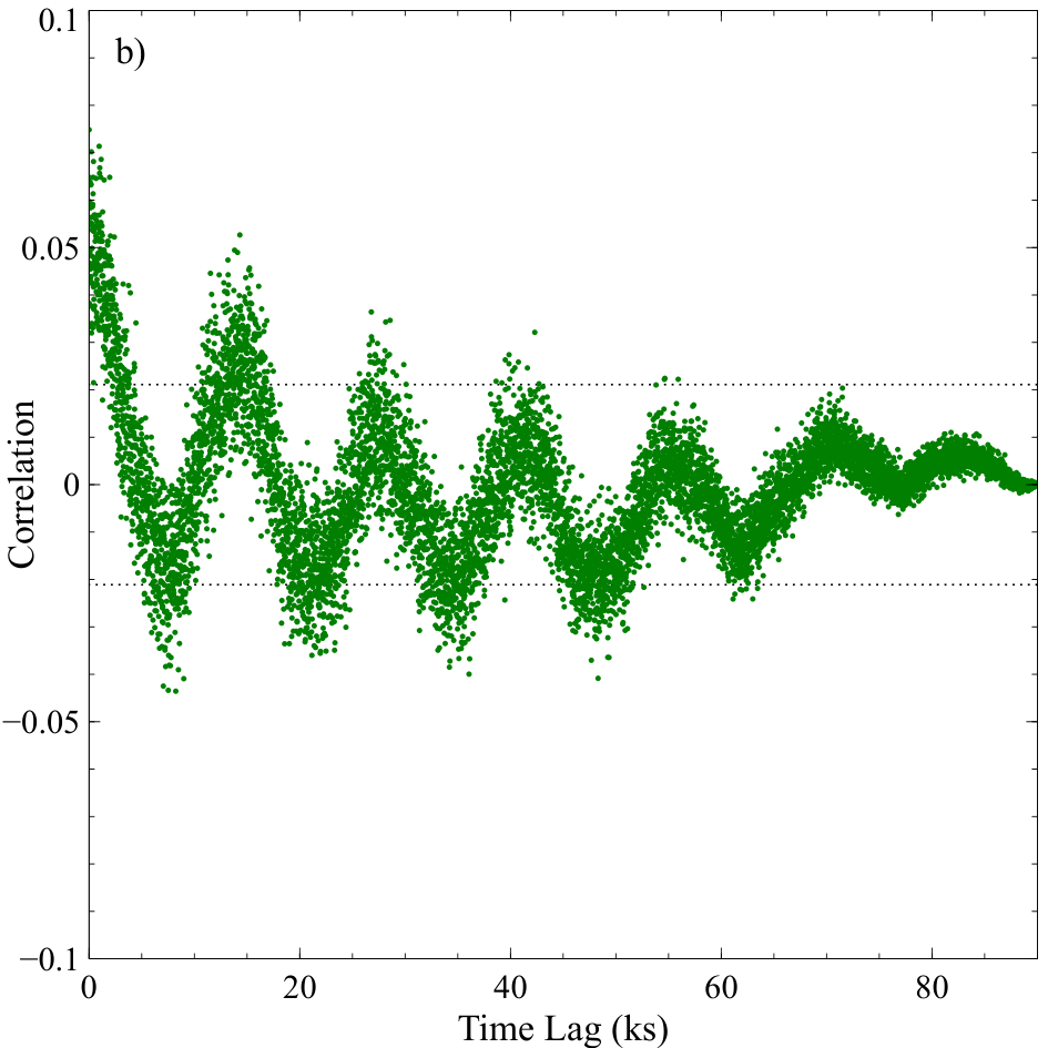
Following the identification of coherent, apparently quasi-periodic, variability in the lightcurves of the observations we consider the use of the autocorrelation to determine the characteristic timescale of variability. The lightcurves for the observations O1 and O2 were processed as described in section 2. Autocorrelation curves were created for both observations using the lightcurves with a time binning of 10s and are shown in figures 2 and 3.
Due to the absence of distinctive peaks in the autocorrelation curves, as seen in the autocorrelation curves for observations of other AGN containing QPEs (see Figure 1), we fit an exponentially damped wave to the autocorrelation function of the form:
| (5) |
in order to find the location of the first peak. This exponentially damped wave provides a good description of the autocorrelation function and has been used in other variability studies of AGN (Chen et al. 2022). See Figure 2b) for an example of the fitting to observation O1. The values of at the first peak of this wave were (13.520.32) ks and (14.350.94) ks for observations O1 and O2 respectively, and were used to create folded lightcurves. The characteristic timescales of variablility are, however, significantly different from those determined by model fitting to the raw lightcurves.
3.3 Folded Lightcurves
| Observation | Model | () | m ( ) | () | (s) | (s) | dof | |
|---|---|---|---|---|---|---|---|---|
| O1 | Wave (QPO) + Constant | – | – | 267 | 1.290 | |||
| O1 | Wave + Linear | – | 266 | 1.285 | ||||
| O1 | Gaussian (QPE) + Constant | – | 266 | 1.283 | ||||
| O1 | Gaussian + Linear | 265 | 1.280 | |||||
| O2 | Wave + Const | – | – | 283 | 0.866 | |||
| O2 | Wave + Lin | – | 283 | 0.864 | ||||
| O2 | Gauss + Const | – | 283 | 0.863 | ||||
| O2 | Gauss + Lin | 282 | 0.865 |
The folded lightcurves were rebinned at a rate of 50s for the purposes of avoiding empty bins during fitting. The best fitting model to the folded lightcurve of O1 was of that of Gaussian bright phases with a linearly decreasing baseline count rate, and the best fitting model to the folded lightcurve of O2 was of that of Gaussian bright phases with a constant quiescent count rate. For observation O1 the full amplitudes (peak to trough) of the wave fit were approximately equal to the baseline rate, while for the Gaussian fits the amplitude was approximately double that of the quiescent rate. For observation O2, the amplitude of the wave oscillations was approximately the magnitude of the baseline count rate, while the amplitudes of the Gaussian profiles were of the same order as the quiescent rate. The fits to the folded lightcurves indicated that the FWHM of the Gaussian bright phases was approximately 50 of the folding timescale. The full details of the parameters for the best fitting models are given in Table 3. The quality of fit was very similar across the four models for each of the observations with very little difference in the reduced chi-squared value within the observations. In all cases where the baseline countrate was modelled by a linear trend the slope of the line was consistent with 0 within 2, and in many cases within one. For the Gaussian model the ratio between the quiescent rate and amplitude decreased from O1 to O2 (four days later), while the duration increased. For the full lightcurves the best fitting sinusoidal and Gaussian profiles for observations O1 and O2 gave quiescent rates and amplitudes of variability which were approximately the same as those found for the folded lightcurves with the exception of the Gaussian fits to O2. In contrast with the fits to the full lightcurves, the amplitudes of variability were less for the second observation in the Gaussian models when compared with the baseline rates, and was smaller. Across the board the reduced chi-squared values were significantly higher when using the full lightcurve over the folded lightcurves, even for similar numbers of degrees of freedom and with a broader time binning.
3.4 Energy Spectra
To determine differences between the spectra during bright and low phases we extracted events for the two observations using selections in time, as making a cut by count rate would be problematic for O2. We defined events during the peaks of the bright phases as being within 25 of from the peak time for each individual bright phase, and events during the low phases as being more than 75 of from the peak time for each individual bright phase. The spectra were then rebinned to ensure there were at least 5 count in each energy bin. We then fit the spectra for energies between 0.2 and 5.0 keV. Fitting each of these spectra to a tbabs bbody model in xspec, with fixed at the Galactic value, indicated that the temperature did not significantly change between O1 and O2, or between the bright and low phases in each observation. The full results are reported in Table 4.
| Obs | Phase | Norm ( | kT (keV) | dof | |
|---|---|---|---|---|---|
| O1 | Bright | 116.17 | 130 | ||
| O1 | Low | 67.19 | 80 | ||
| O2 | Bright | 121.2 | 132 | ||
| O2 | Low | 55.45 | 55 |
4 Discussion
The first QPEs were detected in the active galaxy GSN 069 by Miniutti et al. 2019 in one Chandra and two XMM-Newton observations taken from December 2018 through to February 2019. In the energy range of 0.2–2.0 keV, the QPEs seen in GSN 069 had recurrence times, i.e. the time from the peak of one eruption to the peak of the next, ranging from 29 ks to over 32 ks, and their durations, defined as the full width at half maximum for the best fitting Gaussian curves to the eruptions, ranged between 1.7 ks and 1.9 ks. The size, time and durations of the eruptions did vary when narrower energy bands within this range were also considered. The amplitude of the eruption increased with increasing energy up to the 0.6–0.8 keV band (Miniutti et al. 2019), and then decreased. The durations of eruptions decreased, and the time at which the eruptions peaked was brought earlier, with increasing energy (Miniutti et al. 2019). A previous observation with XMM in 2014 had seen no evidence of QPEs in GSN 069.
QPEs were then detected by Giustini et al. 2020 in the active galaxy RX J1301.9+2747 in an archival XMM observation from 2000 and in a further XMM observation in 2019. The eruptions in this AGN showed many of the same trends as those in GSN 069 including the increasing amplitudes and shorter durations of eruptions in higher energy bands. The eruptions in RX J1301.9+2747 were, however, shorter lived with an average duration of 1.2 ks and they also showed an alternating pattern of larger and smaller amplitude eruptions alongside a pattern of shorter and longer recurrence times between eruptions (20 ks and 13.5 ks).
More recently, QPEs were discovered by Arcodia et al. 2021 in two galaxies whose optical spectra had previously shown no broad line evidence of an accreting black hole. This was achieved by means of a blind search with the eROSITA instrument which were then followed up with observations by XMM-Newton or NICER. The characteristics of the eruptions from the galaxies 2MASS 02314715-1020112 and 2MASX J02344872-4419325 were inconsistent with the predictions from radiation-pressure-driven instability models based on the eruptions seen from the two AGN and widened the temporal parameters of observed QPEs. A further object, XMMSL1 J024916.6-041244, was determined by Chakraborty et al. 2021 to exhibit one full eruption and possibly the start of a second in an archival XMM observation from 2006. There was no such activity in a follow-up observation from August 2021, and as such the quasi-periodicity of any eruptions is unclear.
In this analysis we have considered the use of the autocorrelation function in determining characteristic timescales of variability in an AGN, and have attempted to characterise the variability observed by fitting folded and unfolded lightcurves.
The autocorrelation function plots to the two observations of 2XJ1231 have presented two different characteristic timescales for variability: 13.52 ks for O1, and 14.35 ks for O2. The value of 13.71 ks as previously determined by Lin et al. 2012 is consistent within the errors determined by our analysis for both observations. Our value for the timescale for O1 is not, however, reconcilable with that found by Terashima et al. 2012 of 14.0 ks for the same observation. In both cases in the literature the timescale of variability was determined by means of a blind search in a comparison between folded lightcurves and a constant model. While it is possible, within the errors we have determined, for the timescale of variability to be constant there are indications that it is increasing as time passes, as was confirmed by the increased values for in the sinusoidal and fixed Gaussian models in 2. There were indications of an increasing recurrence time in early observations of GSN 069, as noted by Miniutti et al. 2019, however further analysis of GSN 069 has revealed a more complex picture, with subtly modulating recurrence times within observations (Miniutti et al. 2022). There is, however, a clearly different profile for the autocorrelation functions seen for the lightcurves of the two observations of 2XJ1231 in Figures 2 and 3 when compared with those for lightcurves which definitely contain QPEs, as in the case of Figure 1. The peaks seen in Figure 1 are narrow, well separated and reach high levels of correlation, with the first two peaks in the autocorrelation plot of observation 0831790701 of GSN 069 being above 0.5. In contrast, the features seen in figures 2 and 3 are much broader and of a lower magnitude. The value for the autocorrelation plot of O1 has a magnitude of 0.041 for = 13.52 ks, and the value of the autocorrelation for O2 is 0.037 where = 14.35 ks, as the first peaks of the fitted models to the autocorrelation functions, although the highest values in nearby points are over 0.05 and 0.04 for O1 and O2 respectively. The lower and broader peaks in the autocorrelation function confirm what is seen in the lightcurves; the variability seen is of a lower magnitude and with a higher proportion for the duty cycle () than that seen in observations where QPEs have previously been confirmed to be present. This also accounts for the strong anti-correlation seen at values of , which is not seen in the autocorrelation plots for observations with confirmed QPEs due to the longer periods of quiescence between eruptions in observations of other objects. For both observations, the peaks at are significant at more than 5 (a confidence interval of 0.999999), with the significance levels for observations O1 and O2 being set at 0.0251 and 0.0211 respectively, calculated using the classical test for significance in the autocorrelation function as where CI is the confidence interval, and is the number of points in the lightcurve. This is complemented by the work of Lin et al. 2013, where they determined using power spectra, and simulations of power law and broken power-law models, that a significant signal could be detected to . We also confirmed the significance to a high degree by simulating 1000 lightcurves for each observation using the method outlined by Done et al. 1992 with underlying red-noise power spectra, and computing the autocorrelations of these lightcurves. For O1 97.8 of the autocorrelation functions examined had peaks during the first correlated section after the first zero-crossing time lag at a lower level than that seen for O1, and for O2 the autocorrelation peak was higher than in 96.7 of the simulated lightcurves. The autocorrelation plots of O1 and O2 also contain strong periodic peaks at multiples of a given time lag which further point to a significant periodicity. A manual inspection of the of simulated lightcurves which had stronger individual autocorrelation peaks than that observed in O1 showed that none also had periodic signals, and the peaks were isolated. As such, we can report the significance of the four peaks seen in the autocorrelation plot of O1 to greater than 99.9 significance. A similar inspection of the of simulated lightcurves which had stronger individual autocorrelation peaks than that observed in O2 showed four with further peaks approximately located at time lags that were multiples of the first peak. As such, we can report the significance of the five peaks seen in the autocorrelation plot of O2 to greater than 99.6 significance.
The fitting to the folded lightcurves for both observations of 2XJ1231 showed only marginal differences in the goodness of fit when using a sinudoidal or Gaussian model, which became much greater when modelling the full lightcurves. For the folded lightcurves, the best fitting models were of Gaussian bright phases with a linearly decreasing and constant quiescent rate for observations O1 and O2 respectively. In the best Gaussian models the magnitudes of the bright phases, as the ratio of amplitude to quiescent rate (), were 2.12 and 1.29 for observations O1 and O2, and the bright phases comprised 48.4 and 46.6 of the duty cycle, as the ratio of the duration and the recurrence time. These values for the duty cycle, while higher than any previously seen in QPE candidates, are not too dissimilar to one of those found by Arcodia et al. 2021 where one of the two galaxies exhibiting QPEs (eRO-QPE1) had a duty-cycle of 41. The values for the magnitudes of the bright phases which were determined in these full-band, folded, lightcurves are lower than any others seen in the literature. The reduced chi square values for the model fits to the two observations indicate that all of the models are significant at the 95 level for O2, but none are significant at even the 1 level for O1. Within the observations there is no significant difference in the -values for the models tested and all give approximately the same quality of fit.
When fitting the models to the full lightcurves the goodness of fit was significantly reduced for the wave and Gaussian models when compared with the fitting to the folded lightcurves, and was not at a significant level even once the features of individual Gaussian bright phases were allowed to vary, although it was reduced significantly (reduced by 23.1 for O1 and by 15.3 for O2 on the next best performing models for approximately a 5 reduction in the degrees of freedom). While these reduced chi-square values are high they are not unreasonably higher than those which are achieved by fitting the variable Gaussian model with a linear baseline to observations which are known to contain eruptions: fit to observation 0831790701 of GSN 069 (Figure 10) with five eruptions had =26.5 for 534 degrees of freedom; fit to observation 0851180501 of RX J1301.9+2747 (Figure 11) with three eruptions had =5.37 for 169 degrees of freedom. There were differences noted between the fits to the folded and the full lightcurves for , and . The Gaussian model when fit to the full lightcurves gave a slightly larger amplitude for bright phases than when applied to the folded observations. The amplitude of the bright phases for O1 and O2 (as ) were 2.60 and 3.46. The durations of bright phases were found to be shorter in O1 and longer in O2 than found with the folded fits. In order to provide a fair comparison between the sinusoidal model and another of equivalent complexity we then considered the fixed Gaussian model, and in the case of both observations the Gaussian model provided a better fit to the data than the sinusoidal model. The sinusoidal and fixed Gaussian models fit to O1 both underestimated the recurrence time against the results of the autocorrelation and those quoted in literature with the variable Gaussian model being the most accurate albeit with far larger uncertainties. For O2 all three models underestimated the recurrence time as per the results of the autocorrelation function, even beyond the uncertainties quoted, although the variable Gaussian model was consistent with the value for the recurrence time of 13.71 ks as quoted by Lin et al. 2013. This could be indicative of a significantly varying recurrence time, as has already been seen in the eruptions of RX J1301.9+2747 where the recurrence time varies between 13.5 ks and 20.0 ks (Giustini et al. 2020) and eRO-QPE1 which exhibits eruptions with a mean recurrence time of ks. We then isolated each of the three factors which were allowed to vary in the variable Gaussian model in order to determine if one of them was more significant than the other two. For observation O1 (and O2) the values for were 4.68, 4.49 and 4.53 (4.61, 4.57 and 5.44) when A, and were the only features which were allowed to vary between bright phases in the same observation with a constant quiescent count rate. In both cases the most important feature to the quality of the fit was , but all three had a significant impact on the quality of fit for both observations.
Given that the profile of variability favours the Gaussian model over the sinusoidal model we now consider whether the variability seen fits the features of QPEs seen in other objects. The timescales of variability seen in 2XJ1231 are within the ranges of values seen in other QPE host objects. The average (and standard deviation on) is ks, which is greater than that seen for eRO-QPE2, 8.640.30 ks (Arcodia et al. 2021), and more than 80 of the average recurrence time seen in RX J1301.9+2747, being 16.53.5 ks (Giustini et al. 2020), although it is considerably shorter than those seen in GSN 069 and eRO-QPE1, being 32.22.1 ks and 66.69.7 ks (Miniutti et al. 2019; Arcodia et al. 2021). The average of (and standard deviation on) the duration of bright phases seen in 2XJ1231, 7.001.45 ks, is also within the range of values for seen in other objects. The largest duration for eruptions previously seen was in eRO-QPE1 at 27.43.6 ks (Arcodia et al. 2021), this object also having the longest recurrence time between durations. 2XJ1231 does display the largest duty cycle () amongst any of the objects considered so far, with in O1 and in O2, the next largest being for eRO-QPE1.
As has already been remarked (Ho et al. 2012; Lin et al. 2013; Terashima et al. 2012, etc.), 2XJ1231 has a very low black hole mass, . We therefore consider the possibility that the variability seen in 2XJ1231 may be the result of the same mechanism which drives QPEs in other objects, but around a less massive black hole. In Figure 6 we show the distribution of (Wevers et al. 2022) and (Miniutti et al. 2019; Giustini et al. 2020; Arcodia et al. 2021) for QPE host AGN and 2XJ1231. We consider linear relationships between the mass and recurrence time under the assumption that timescales of variability could be dependent on black hole mass, in the case of thermal-viscous instabilities, or due to preferable radii around the central black holes which would scale with mass.
The best fitting relationship between and as determined by these five objects, see Fig.6, was
| (6) |
where ks and ks/ , although this has been heavily affected by the possible outlier RX J1301.9+2747, which deviates from the general trend for longer recurrence times being associated with higher black hole masses. The long-term evolution of QPE timing properties will remain unclear, even if 2XJ1231 were to be considered a candidate. QPEs are clearly a transient phenomena in at least some of the sources already identified, with QPEs appearing and then disappearing in GSN 069, with a lifetime between 1 and 5.5 years (Miniutti et al. 2022). Conversely, if the eruptions detected in observations of RX J1301.9+2747 have continued between observations then the lifetime could be of the order of decades. The variability seen in 2XJ1231 ’switched on’ at some point between an observation in 2003 and those analysed above, and further observations would be needed to place limits on its lifetime.
Several of the energy-dependent features of QPEs have been identified through the examination of eruptions in GSN 069 (Miniutti et al. 2019) and RX J1301.9+2747 (Giustini et al. 2020), and are outlined above. We therefore consider the energy-dependent characteristics of the variability seen in 2XJ1231, using three energy bands 0.2–0.5 keV, 0.5–1.0 keV, and 1–2 keV. The lightcurves and best fitting models are shown in figures 7 and 8. Details of the fits to the folded and full lightcurves are given in tables 5 and 6 respectively. Given the super-soft nature of the spectrum, as previously identified by Lin et al. 2013 and Terashima et al. 2012 it is unsurprising that the variability in the highest energy band was dominated by noise (as was also noted in observations of GSN 069 above 2keV Miniutti et al. 2019 and above 1.3keV for RX J1301.9+2747 by Giustini et al. 2020) and the fitter failed in both cases to satisfactorily fit the variable Gaussian model to the observed lightcurve. The lack of clear variability in the highest energy band observed does, however, continue to suggest that the variability seen in 2XJ1231 may indeed be indicative of the presence of QPEs in the lower energy ranges. The effect of this band is to suppress the magnitude of variablility when viewed over a broader energy range. As such, the average amplitude of variability () found using the variable Gaussian model in the 0.2-1.0keV energy band is 2.860.45 for O1 and 8.561.14 for O2.
| Obs. | Energy (keV) | (s) | (s) | |
|---|---|---|---|---|
| O1 | 0.2-0.5 | 9.705.76 | 677070 | 7790220 |
| O1 | 0.5-1.0 | 1.650.17 | 693010 | 518010 |
| O1 | 1.0-2.0 | 0.3010.204 | 85207040 | 302040 |
| O2 | 0.2-0.5 | 1.570.20 | 4570140 | 5920390 |
| O2 | 0.5-1.0 | 14.718.8 | 5040120 | 10000100 |
| O2 | 1.0-2.0 | 1.532.92 | 62304070 | 500010 |
The fits to the folded lightcurves do, at times, show the energy-dependent characteristics of QPEs which have been seen in other objects. In observation O1 the durations of bright phases appear to decrease in time as the energy band increases, and is also seen in the highest and lowest energy bands in O2, with the 0.5-1.0 keV band being an exception. We also observe a much larger amplitude for bright phases in O2 in the 0.5-1.0 keV band as opposed to the bright phases in the 0.2-0.5 keV band. Contrary to observations of GSN 069 and RX J1301.9+2747, however, the bright phases appear to occur later with increasing energy, as opposed to earlier (Miniutti et al. 2019; Giustini et al. 2020). There is a similarly unclear pattern of results when considering the fits to the full lightcurves, with the amplitude decreasing with energy in O1 and the reverse seen in O2. Additionally, is lowest in the 0.5-1.0keV band in O1, but the durations of bright phases increases with energy in O2. Such energy-dependent behaviour is contrary to that which is seen in other QPE sources (Miniutti et al. 2019; Giustini et al. 2020).
The highly energy dependent amplitudes of the eruptions seen in 2XJ1231 are of a generally lower size than those seen in other QPE host objects, although this is very much energy dependent. The amplitudes of eruptions vary between 2 and 100 in the 0.2-0.3 keV and 0.6-0.8 keV bands in GSN 069, between 2 and 100 in the 0.2-0.3 keV and 1.0-1.3 keV bands in RX J1301.9+2747, and the ratio of peak to quiescent 0.001-100 keV disk luminosities in eRO-QPE1 and eRO-QPE2 are 294 and 11 respectively. The amplitudes of the eruptions reaching as much as a factor of ten in 2XJ1231 would therefore widen the parameter space for known QPE sources should this indeed be considered as the fifth QPE host object.
| Obs. | Energy (keV) | (s) | ||
|---|---|---|---|---|
| O1 | 0.2-0.5 | 0.0160.005 | 4.871.26 | 6720520 |
| O1 | 0.5-1.0 | 0.0120.002 | 4.471.08 | 671010 |
| O1 | 1.0-2.0 | 0.0110.001 | 0.840.51 | 7630150 |
| O2 | 0.2-0.5 | 0.0170.001 | 2.680.53 | 4440480 |
| O2 | 0.5-1.0 | 0.0080.001 | 4.00.9 | 4980180 |
| O2 | 1.0-2.0 | 0.0100.001 | 0.100.16 | 6230400 |
The temperature of the disk, as determined by the spectral fitting reported in section 3.4, does not change within errors, neither across observations nor during the different bright and low phases. Instead, we observe a significant change in the normalisation, indicating that the variability may be due to a change in the area of the radiating region, rather than in the temperature of the radiative material. This is in contrast with spectral fitting to other QPE objects, which show transitions from cooler states during quiescence to hotter states during eruptions (Miniutti et al. 2019; Giustini et al. 2020; Chakraborty et al. 2021; Arcodia et al. 2021), with typical temperature differences between quiescent and eruptive states being eV. The temperature is closer to that associated with the eruptive phases of QPE hosts, and so the absence of temperature changes may be caused by the lack of real quiescent states in 2XJ1231 caused by broader, overlapping bright phases. It is notable that this temperature is also comparable to that of the soft excess seen in AGN.
Ultimately, the analysis we can perform is limited by the brightness of the source and the sensitivity of detectors and observations. The available observations are less than the limit of what is possible with regards to the exposure time and XMM orbit restrictions, but given that we have already observed a considerable number of variability cycles we should focus on obtaining pointed observations, rather than those where the source is a long way off-axis, which might improve the data and allow MOS1 to be used. Given the super-soft nature of the source spectrum it is likely that we are approaching the limits of what can be learned about 2XJ1231 using XMM unless it becomes significantly brighter, which would seem unlikely given that follow-up Swift and Chandra observations (Lin et al. 2017) indicate that the source is becoming fainter. If this decrease in luminosity is due to the long-term evolution of a tidal disruption event (TDE) it could indicate that the variability seen in 2XJ1231 has a similar cause to that seen in GSN 069 and XMMSL1 J024916.6-041244, both of which are considered to contain QPEs, and which are both strong TDE candidates (Chakraborty et al. 2021; Miniutti et al. 2022). If this is the case we might expect to see a re-brightening as the variability seen in O1 and O2 disappears as has been observed in GSN 069 (Miniutti et al. 2022).
Given the ambiguous nature of these results we then conducted a manual, targeted search for other AGN which might contain QPEs in the XMM archive. To determine a sample of AGN to look at in greater detail we used some of the criteria which were used to identify RX J1301.9+2747 and 2XJ1231 as possible QPE candidates. To find AGN which meet these criteria we used two freely-available enhanced catalogues CHANSNGCAT22 2 https://heasarc.gsfc.nasa.gov/W3Browse/all/chansngcat.html (She et al. 2017), and Optical Emission Line Properties and Black Hole Mass Estimates for SPIDERS DR14 AGN33 3 https://www.sdss.org/dr15/data_access/value-added-catalogs/?vac_id=optical-emission-line-properties-and-black-hole-mass-estimates-for-spiders-dr14-agn (Coffey et al. 2019). Making an initial selection based only on , as determined using the relationship for CHANSNGCAT and using spectral lines for SPIDERS DR14 AGN, gave a very restrictive sample, with only 17 AGN with identified in the CHANSNGCAT catalogue, and none below that threshold in the SPIDERS catalogue (with being the lowest). From the 17 AGN identified using CHANSNGCAT we found 11 objects which had a combined 51 observations in the XMM archive, details of which are presented in Table 7 in Appendix A. The observations were processed in the same manner as for the observations of 2XJ1231 analysed above, and lightcurves from the EPIC pn instrument for events from 0.2-2.0keV and associated autocorrelation plots were produced. In none of the lightcurve or autocorrelation plots for any of the 51 observations of these 11 objects were there any features which indicated the possible existence of QPEs. Although this search was only performed on a very select sample it suggests that variability of the kind seen in GSN 069, RX J1301.9+2747, eRO-QPE1, eRO-QPE2, and 2XJ1231 is not a given feature of all lower-mass AGNs and may be even more unusual than previously thought.
5 Conclusions
The variability seen in the low-mass, super-soft AGN 2XMM J123103.2+110648 remains somewhat ambiguous in nature. We have successfully applied the autocorrelation function to identify characteristic timescales for the variablity, and found values which are consistent with those determined by other means as quoted in the literature. The profiles of the autocorrelation plots were different in appearance to those seen for observations with confirmed QPEs, being less pronounced, but the features seen were still statistically significant at 5, with = 13.52 ks and 14.35 ks for O1 and O2 respectively. This analysis has shown that the autocorrelation function can be applied in finding QPE-like behaviour, and as such it should be considered as a viable tool in further attempts to find more objects which could contain QPEs.
We have considered the profile of the variability seen using a number of measures and find that they point towards the variability in 2XJ1231 being a QPE in nature. We determined from the best fitting variable QPE models that the amplitudes (as /), recurrence times and durations of eruptions in a 0.2–2.0 keV energy range were 2.60 (3.46), 13.7 ks (13.7 ks), and 6.17 ks (7.69 ks) respectively for O1 (and O2). The profile of the variability is best described by a series of Gaussian eruptions, and although the models provide a reasonable fit, they are too rudimentary to fully describe the behaviour. We have observed that the baseline rate is likely more complex than a linear trend, and indeed the fit to observation 0831790701 of GSN 069 (see Figure 10) is suggestive of an oscillating quiescent count rate with there also being an indication of a QPO during the quiescent periods of RX J1301.9+2747 (Song et al. 2020). A brief examination of the possibility of an oscillating baseline count rate for the Gaussian models significantly improved the fit to O2, however there was no improvement in the fit quality for O1. For O1, the inclusion of an oscillating baseline resulted in for 234 degrees of freedom, while for O2 the fit improved, with for 334 degrees of freedom. This fit to O2 is shown in Figure 9. 2XJ1231 would be the lowest mass AGN should it be the fifth member of the newly discovered class of QPE host galaxies.
We have purposely taken an agnostic approach to this profiling with regards to the cause or method by which eruptions could be created in order to not prejudice the identification of the features which we have identified. In now considering some of the models which have previously been proposed by others to explain QPE phenomena we find that:
- •
While the case against gravitational lensing, as described by Ingram et al. 2021, for the mechanism in QPE sources is strong in light of the asymmetry seen in the eruptions of eRO-QPE1 (Arcodia et al. 2022), we can make no similar claim for the variability in 2XJ1231. It does, however, still appear to be an unlikely mechanism, as with GSN 069 and RX J1301.9+2747, as the black hole mass being as low as would produce eruptions which are either not of a large enough amplitude or not long enough in duration without the inclusion of a complex geometry for the emitting regions.
- •
An accretion flow instability, following the same methodology as applied by Arcodia et al. 2021 and outlined in Grzedzielski et al. 2017, for the observation O2, with amplitude, as the ratio of the unabsorbed 0.5–2.0 keV luminosities in the high and low flux states (Terashima et al. 2012) as a proxy for the bolometric luminosities, , duty cycle , and recurrence time ks gives a value for the viscosity parameter of for . While this value for is not unfeasibly high it would increase with a less conservative estimate for the amplitude of the eruptions.
- •
Accretion from a compact companion object, as described by King 2020, would imply that the orbiting companion is a white dwarf of mass in an highly eccentric orbit with . The pericentre for such an orbit would be at . This mechanism would raise further questions as to the high duty-cycle seen in the variability of 2XJ1231. If we were to consider the possibility of a less eccentrically orbiting companion, which would be accreting for a greater proportion of its orbit, rather than just at pericentre passage, we might expect to see a smoother transition between the high and low states, and a greater duty cycle such as is seen in 2XJ1231. Whether this could be extended further to explain the behaviour of QPO hosts is unclear.
We have also examined a wider population of other low-mass AGN, with eleven objects identified as having , and examined 47 XMM observations of these objects. We found no evidence of QPE-like behaviour in examinations of the lightcurves and autocorrelation plots of these observations over a range of time-binning space.
The immediate aims for further work with 2XJ1231 should include
- •
Obtaining more targeted observations in order to provide better quality lightcurves with higher SNR.
- •
Applying more complex models to the variability seen to better profile the behaviour of 2XJ1231.
In moving forward we also need to consider how to appropriately distinguish between quasi-periodic oscillations and eruptions, or indeed whether they are in fact different manifestations of the same phenomenon. Does the variability seen in 2XJ1231 represent an intermediate point on the QPO/QPE continuum? We have considered the profiling of lightcurves as a possible mechanism, but other parametric measures should also be considered if a distinction between the two pheomena is necessary. Continued monitoring of the other QPE host objects to determine how their QPEs evolve over time will also help to build a fuller understanding of quasi-periodic eruptions, how they fit into our understanding of AGN, and of how 2XJ1231 fits into our understanding of quasi-periodic eruptions.
Acknowledgements
All figures in this paper were created using Veusz. This work is supported by the UKRI AIMLAC CDT, funded by grant EP/S023992/1. We sincerely thank the anonymous referee for their thoughtful and constructive report which improved the quality of this paper.
Data Code Availability
All data used in this analysis is freely available in the XMM Newton Science Archive (http://nxsa.esac.esa.int/nxsa-web/#home). This analysis used the stingray module for python version 0.3 and all code and data analysis products are available on GitHub upon request. For the purpose of open access, the author has applied a Creative Commons Attribution (CC BY) licence [where permitted by UKRI, ‘Open Government Licence’ or ‘Creative Commons Attribution No-derivatives (CC BY-ND) licence’ may be stated instead] to any Author Accepted Manuscript version arising
References
- Arcodia et al. (2021) Arcodia R., et al., 2021, Nature, 592, 704
- Arcodia et al. (2022) Arcodia R., et al., 2022, Astronomy & Astrophysics, 662, A49
- Chakraborty et al. (2021) Chakraborty J., Kara E., Masterson M., Giustini M., Miniutti G., Saxton R., 2021, The Astrophysical Journal Letters, 921, L40
- Chen et al. (2022) Chen Y.-J., et al., 2022, doi:10.48550/arxiv.2206.11497
- Coffey et al. (2019) Coffey D., et al., 2019, Astronomy and Astrophysics, 625, A123
- Done et al. (1992) Done C., Madejski G. M., Mushotzky R. F., Turner T. J., Koyama K., Kunieda H., 1992, The Astrophysical Journal, 400, 138
- Edelson et al. (2002) Edelson R., Turner T. J., Pounds K., Vaughan S., Markowitz A., Marshall H., Dobbie P., Warwick R., 2002, The Astrophysical Journal, 568, 610
- Edelson et al. (2019) Edelson R., et al., 2019, The Astrophysical Journal, 870, 123
- Fukumura et al. (2010) Fukumura K., Shrader C. R., Dong J. W., Kazanas D., 2010, Astronomy and Astrophysics, 524, A34
- Gandhi et al. (2008) Gandhi P., et al., 2008, Monthly Notices of the Royal Astronomical Society: Letters, 390, L29
- Giustini et al. (2020) Giustini M., Miniutti G., Saxton R. D., 2020, Astronomy and Astrophysics, 636, L2
- Gliozzi et al. (2002) Gliozzi M., Brinkmann W., Räth C., Papadakis I. E., Negoro H., Scheingraber H., 2002, Astronomy and Astrophysics, 391, 875
- Grzedzielski et al. (2017) Grzedzielski M., Janiuk A., Czerny B., Wu Q., 2017, Astronomy & Astrophysics, 603, A110
- Gupta et al. (2018) Gupta A. C., Tripathi A., Wiita P. J., Gu M., Bambi C., Ho L. C., 2018, Astronomy and Astrophysics, 616, L6
- Ho et al. (2012) Ho L. C., Kim M., Terashima Y., 2012, The Astrophysical Journal Letters, 759, L16
- Huppenkothen et al. (2019) Huppenkothen D., et al., 2019, The Astrophysical Journal, 881, 39
- Ingram et al. (2021) Ingram A., Motta S. E., Aigrain S., Karastergiou A., 2021, Monthly Notices of the Royal Astronomical Society, 503, 1703
- King (2020) King A., 2020, Monthly Notices of the Royal Astronomical Society: Letters, 493, L120
- Lin et al. (2012) Lin D., Webb N. A., Barret D., 2012, The Astrophysical Journal, 756, 27
- Lin et al. (2013) Lin D., Irwin J. A., Godet O., Webb N. A., Barret D., 2013, Astrophysical Journal Letters, 776, L10
- Lin et al. (2014) Lin D., Webb N. A., Barret D., 2014, The Astrophysical Journal, 780, 39
- Lin et al. (2017) Lin D., Godet O., Ho L. C., Barret D., Webb N. A., Irwin J. A., 2017, Monthly Notices of the Royal Astronomical Society, 468, 783
- McHardy et al. (2004) McHardy I. M., Papadakis I. E., Uttley P., Page M. J., Mason K. O., 2004, Monthly Notices of the Royal Astronomical Society, 348, 783
- Metzger et al. (2022) Metzger B. D., Stone N. C., Gilbaum S., 2022, The Astrophysical Journal, 926, 101
- Miniutti et al. (2019) Miniutti G., et al., 2019, Nature, 573, 381
- Miniutti et al. (2022) Miniutti G., Giustini M., Arcodia R., Saxton R. D., Read A. M., Bianchi S., Alexander K. D., 2022, Astronomy and Astrophysics
- Mushotzky et al. (1993) Mushotzky R. F., Done C., Pounds K. A., 1993, Annual Review of Astronomy and Astrophysics, 31, 717
- Musoke et al. (2022) Musoke G., Liska M., Porth O., van der Klis M., Ingram A., 2022, doi:10.48550/arxiv.2201.03085
- Raj & Nixon (2021) Raj A., Nixon C. J., 2021, The Astrophysical Journal, 909, 82
- Reis et al. (2012) Reis R. C., Miller J. M., Reynolds M. T., Gültekin K., Maitra D., King A. L., Strohmayer T. E., 2012, Science, 337, 949
- She et al. (2017) She R., Ho L. C., Feng H., 2017, The Astrophysical Journal, 835, 223
- Song et al. (2020) Song J. R., et al., 2020, Astronomy & Astrophysics, 644, L9
- Terashima et al. (2012) Terashima Y., Kamizasa N., Awaki H., Kubota A., Ueda Y., 2012, Astrophysical Journal, 752, 154
- Ulrich et al. (1997) Ulrich M. H., Maraschi L., Urry C. M., 1997, Annual Review of Astronomy and Astrophysics, 35, 445
- Vaughan (2010) Vaughan S., 2010, Monthly Notices of the Royal Astronomical Society, 402, 307
- Wevers et al. (2022) Wevers T., Pasham D. R., Jalan P., Rakshit S., Arcodia R., 2022, Astronomy and Astrophysics, 659, L2
- Xian et al. (2021) Xian J., Zhang F., Dou L., He J., Shu X., 2021, The Astrophysical Journal Letters, 921, L32

Appendix A Appendix A - QPE Candidate search
Table 7 contains a list of all XMM observations of QPE candidate galaxies which were processed and analysed for evidence of QPEs. In all cases the pn lightcurves were binned at multiples of 10s for all values between 10s and 500s, to account for shot-noise in lower count rate observations, and associated autocorrelation plots were created at all time bin values. In none of the observations listed was any QPE-like behaviour observed.
| AGN Name | OBSID | Exposure (ks) | |
|---|---|---|---|
| NGC1331 | 5.48 | 0304190101 | 65.9 |
| NGC3367 | 5.64 | 0551450101 | 31.4 |
| NGC3599 | 5.85 | 0411980101 | 6.9 |
| – | – | 0556090101 | 43.6 |
| NGC4467 | 5.86 | 0112550601 | 24.6 |
| – | – | 0200130101 | 111.0 |
| – | – | 0510011501 | 10.1 |
| – | – | 0761630101 | 118.0 |
| – | – | 0761630201 | 118.0 |
| – | – | 0761630301 | 117.0 |
| NGC4476 | 5.58 | 0114120101 | 60.1 |
| – | – | 0200920101 | 109.3 |
| – | – | 0551870401 | 21.6 |
| – | – | 0551870601 | 21.3 |
| – | – | 0603260201 | 17.9 |
| – | – | 0803670501 | 132.0 |
| – | – | 0803670601 | 65.0 |
| – | – | 0803671001 | 63.0 |
| – | – | 0803671101 | 131.9 |
| NGC4559 | 5.14 | 0152170501 | 42.2 |
| – | – | 0842340201 | 75.4 |
| NGC4654 | 5.07 | 0651790201 | 28.9 |
| NGC5273 | 5.97 | 0112551701 | 17.1 |
| – | – | 0805080401 | 110.9 |
| – | – | 0805080501 | 28.0 |
| NGC6946 | 5.43 | 0093641201 | 8.5 |
| – | – | 0093641501 | 8.6 |
| – | – | 0093641601 | 10.1 |
| – | – | 0093641701 | 11.3 |
| – | – | 0200670101 | 16.4 |
| – | – | 0200670201 | 14.4 |
| – | – | 0200670301 | 15.6 |
| – | – | 0200670401 | 21.2 |
| – | – | 0401360101 | 20.9 |
| – | – | 0401360201 | 24.4 |
| – | – | 0401360301 | 24.4 |
| – | – | 0500730101 | 31.9 |
| – | – | 0500730201 | 37.3 |
| – | – | 0691570101 | 119.3 |
| – | – | 0794581201 | 50.0 |
| – | – | 0870830101 | 17.9 |
| – | – | 0870830201 | 17.7 |
| – | – | 0870830301 | 16.0 |
| – | – | 0870830401 | 17.8 |
| NGC7314 | 5.59 | 0111790101 | 44.7 |
| – | – | 0311190101 | 83.9 |
| – | – | 0725200101 | 140.5 |
| – | – | 0725200301 | 132.1 |
| – | – | 0790650101 | 65.0 |
| NGC925 | 6.0 | 0784510301 | 50.0 |
| – | – | 0862760201 | 42.0 |
Appendix B QPE Model Fits to GSN 069 and RX J1301.9+2747
Figures showing the QPE model fits, with variable features and linearly increasing (zero within errors) baseline count rate for observations 0831790701 of GSN 069 and 0851180501 of RX J1301.9+2747. Lightcurves were binned at a rate of 250s for fitting and are presented with time bins of 1 ks.