Influential Recommender SystemThanks: Pengfei Zhao is the corresponding author.
Abstract
Traditional recommender systems are typically passive in that they try to adapt their recommendations to the user’s historical interests. However, it is highly desirable for commercial applications, such as e-commerce, advertisement placement, and news portals, to be able to expand the users’ interests so that they would accept items that they were not originally aware of or interested in to increase customer interactions. In this paper, we present Influential Recommender System (IRS), a new recommendation paradigm that aims to proactively lead a user to like a given objective item by progressively recommending to the user a sequence of carefully selected items (called an influence path). We propose the Influential Recommender Network (IRN), which is a Transformer-based sequential model to encode the items’ sequential dependencies. Since different people react to external influences differently, we introduce the Personalized Impressionability Mask (PIM) to model how receptive a user is to external influence to generate the most effective influence path for the user. To evaluate IRN, we design several performance metrics to measure whether or not the influence path can smoothly expand the user interest to include the objective item while maintaining the user’s satisfaction with the recommendation. Experimental results show that IRN significantly outperforms the baseline recommenders and demonstrates its capability of influencing users’ interests.
I Introduction
Recommender system (RS) has created huge business values for applications such as e-commerce, advertising, and streaming media. Traditional RS tries to learn users’ internal interests from their historical user-item interactions and recommend items judged to be relevant to the users’ interests. Despite the recent advancements of RS in modeling the users’ long/short-term interests, most existing works on RSs are passive in that their recommendations are driven by users’ historical interests. If the user does not respond to a recommendation positively, these RSs would try to please the user by selecting another item that better fits the user’s interest. In other words, they model the users’ interests and fit their recommendations to the user’s internal interests instead of proactively developing their external interests. We refer to this RS approach as User-oriented Recommender System (URS).
For many commercial applications, a business may want its recommendation system to be able to influence users to like an objective item that they originally may not be interested in by expanding the users’ current interests. This allows a business to develop effective branding and marketing strategies by enticing users to pay attention to some promotional or new-arrival items. A URS would not be able to achieve this goal since it only displays items within the users’ interests. On the other hand, a straightforward advertisement placement system will simply display the objective items to the users, amounting to hard-selling the items to the users. Neither is desirable from a business or user point of view. In this paper, we propose a new RS paradigm named Influential Recommender System (IRS). IRS aims to influence a user ’s interest towards a given objective item by recommending a sequential list of items (called influence path), which not only follows ’s historical interests but also progressively broadens ’s interests towards the objective .

Figure 1 illustrates the idea of IRS in a movie recommendation scenario. Solid arrows indicate users’ viewing histories (one color per user), which reflect the users’ chronological behavioral sequences of movie watching. These sequences reflect not only the users’ interests profile but also the movies’ sequential dependencies. In the example, Bob is interested in fantasy movies, with a watch history of The Matrix The Abyss The Terminator Avatar Source Code, in which all movies are of the fantasy genre. Similarly, Tom is a fan of director James Cameron, and Jenny likes romance movies.
Assume that the goal of IRS is to influence Eric to watch the objective movie The Notebook, a classic romance movie. From Eric’s watch history, Inception The Matrix, it is fair to infer that Eric has a high chance of accepting fantasy movies, but how can IRS lead him to watch the romance movie The Notebook?
We notice that Eric and Tom both watched The Matrix. Thus, there is a good chance for Eric to accept Tom’s behavioral sequence, i.e., The Abyss The Terminator Avatar. After Eric accepts Avatar, a romance movie directed by Cameron, we are more confident to say that Eric has developed a certain level of interest in Cameron and the romance genre. Taking one step forward, we can recommend Titanic, another classic romance movie directed by Cameron, to Eric. If Eric accepts it, his interest in romance movies is further strengthened. Following Jenny’s sequence, recommending The Notebook as the next movie for Eric becomes natural and persuasive. This potential recommendation sequence (called influence path) is indicated by the green dash arrows. This example illustrates the goal of IRS, that is, the progressive expansion of a user’s interest towards the objective item along an enticing, smooth influence path learned from the large historical user data.
There are key differences between URS and IRS. For URS, users play the central role, and URS aims to adapt to the users’ historical interests, while for IRS, the platform takes the proactive role to leading the users to like the preset objective items by progressively recommending a carefully selected sequence of items. Filling the gap from URS to IRS presents several challenges. First, the influence path should (i) not deviate too much from the user’s historical interest in order to maintain the user’s trust and satisfaction with the system and (ii) progressively recommend items related to the objective item so that the user’s interest in the objective item can be developed and the transition from the user’s interest towards the objective item is gradual and smooth. Second, user-item interactions have sequential patterns, i.e., the next item/action depends more on items/actions the user engaged in recently [30]. Thus, the generation of an influence path must align with the sequential dependencies among the items. Third, a user’s preference for external influence is personal. That is, some users may be extrovert, i.e., they favor exploration and thus can be easily affected by external influences, but some may favor staying in their comfort zone and are difficult to be persuaded to accept new interests. For the former, influence paths could be more aggressive, i.e., they can deviate more from the users’ existing interests to reach the objective item in fewer steps; for the latter, the reverse should be taken. We introduce the notion of Impressionability to account for the users’ different preferences of external influence.
To meet these challenges, we propose Influential Recommender Network (IRN), which is adapted based on the widely used Transformer model [31] in natural language processing (NLP). Both the user-item interaction sequences and NLP sentences have a sequential structure, and the dependencies among items/words exist not only in adjacent items/words but also among distant items/words, which can be well captured by the multi-head attention mechanism. Furthermore, to accommodate the influence of the objective item and to personalize the generation of the influence path for individual users with different degrees of impressionability, we design a new masking scheme termed Personalized Impressionability Mask (PIM) that incorporates user embedding into the calculation of item attention weights.
To the best of our knowledge, we are the first to propose influential recommendations. Consequently, there are no standard performance metrics or similar approaches to serve as baselines for performance evaluation. To overcome these problems, we design new performance metrics that can be used to measure whether the proposed IRS frameworks can lead the user to the objective item while satisfying the user’s current interest. As explained in Section IV, we need to determine how much a user is interested in an unseen item, which cannot be obtained from offline datasets. Thus, we propose to use an Evaluator to simulate the reaction of a user to an unseen item.
The contribution of this paper is multi-fold:
- 1.
We propose a new paradigm of recommendation named Influential Recommender System (IRS), which proactively leads the user towards a given objective item instead of passively adapting the recommendations to the user’s historical interests. To the best of our knowledge, IRS is the first to infuse proactivity and influence to RSs.
- 2.
We design Influential Recommender Network (IRN), a Transformer-based model to encode the items’ sequential dependencies. In order to model the user’s personalized preference of external influence, we extend Transformer by adding user embedding to the attention mechanism.
- 3.
We design several performance metrics and offline experiments specifically for evaluating IRS. Experimental results show that our proposed IRN significantly outperforms the baseline recommenders and can smoothly and progressively influence a user’s interest.
The remaining parts of the paper are organized as follows. We briefly review the related work in Section II. In Section III, we formulate the problem of IRS and propose three frameworks, including two solutions adapted from existing URS and our Influential Recommender Network. In Section IV, we first introduce the experimental setup and IRS evaluation and then present a detailed discussion of the experimental results. Finally, we conclude our work and summarize the future directions in Section V.
II Related Work
II-A Bayesian Persuasion
There have been decades of studies on how an entity (e.g., person, group, etc.) can be persuaded to change its action [6, 19, 1, 17]. Persuasion can be defined as influencing behavior via the provision of information. Bayesian Persuasion studies the persuasion problem in a rational (Bayesian) manner [19, 4, 18]. The problem can be abstracted as a sender designing a signaling plan with the right amount of information disclosed so as to influence the behaviors of another receiver. Later, extensive works have applied the information design of Bayesian Persuasion to real-world scenarios, such as social learning for online recommendation platform [7], products advertisement [2], and matching markets [27], etc. In this paper, we consider the persuasion problem from the perspective of RS, which aims at changing the user to like an objective item by recommending a selected sequence of items to the user. In contrast to the existing works that model the persuasion problem as an information design and mechanism design problem requiring domain knowledge, our proposed work is data-driven where the persuasion is done by designing an influence path with proper machine learning techniques. To the best of our knowledge, we are the first to integrate RS with persuasion behavior.
II-B Sequential Recommendation System
Given the natural sequential order of user-item interactions, the sequential recommender system (SRS) tries to incorporate sequential signals into the next-item recommendation task. Due to the diversity and complexity of user-item interactions, SRSs have to face several challenges [35]. (1) Learning higher-order long/short-term sequential dependencies. Compared to lower-order sequential, which are relatively simple and can be easily modeled with Markov chain or factorization machines, long/short-term sequential dependencies are much more complex and harder to capture because of their complicated multi-level cascading dependencies crossing multiple user-item interactions. Various approaches such as recurrent neural networks (RNN) based models [38, 14, 5], graph-based models [41, 39, 37] have been applied to SRSs due to their strength in modeling long/short-term interests. (2) Handling user-item interaction sequences with flexible order and noise. [30, 43] exploits the property of convolutional neural networks (CNN) to model the flexible orders of user-item interactions. Attention models have been employed to emphasize relevant and important interactions in a sequence while downplaying irrelevant ones [20, 34, 42, 28]. (3) Handling user-item interaction sequences with heterogeneous relations and hierarchical structures. [29, 36] proposed mixture models to tackle the problem. The difference between SRS and IRS is, SRS models the items’ sequential dependencies for the next-item recommendation task, which belongs to the URS category, while IRS utilizes the sequential dependency information to generate influence paths towards the objective item.
III Influential Recommender System
III-A Problem Definition
In sequential recommender systems, user-item interactions are represented as sequences. For a given dataset, we denote the set of all user-item interaction sequences as , which has size . Each sequence consists of an ordered list of items. All the items occurring in constitute the item set of size . Let denote the set of all users, and denote the set of sequences belonging to . We have , where is the number of users.
The problem of influential recommendation is defined as: given a user ’s viewing history and a selected objective item , produce a sequence of items, named influence path (denoted as ), which starts from ’s original interests and leads towards progressively and smoothly. Figure 2 illustrates the idea. An influence path aims to meet two criteria: a path item should expand the user’s interests toward the objective and simultaneously satisfy the user’s current interests so that the user will not lose patience to the recommendations. The smoothness of the path is also critical since an abrupt recommendation may upset the user. Note that can be picked according to the needs of the specific application. In this work, we use random to avoid the bias incurred by manual selection.
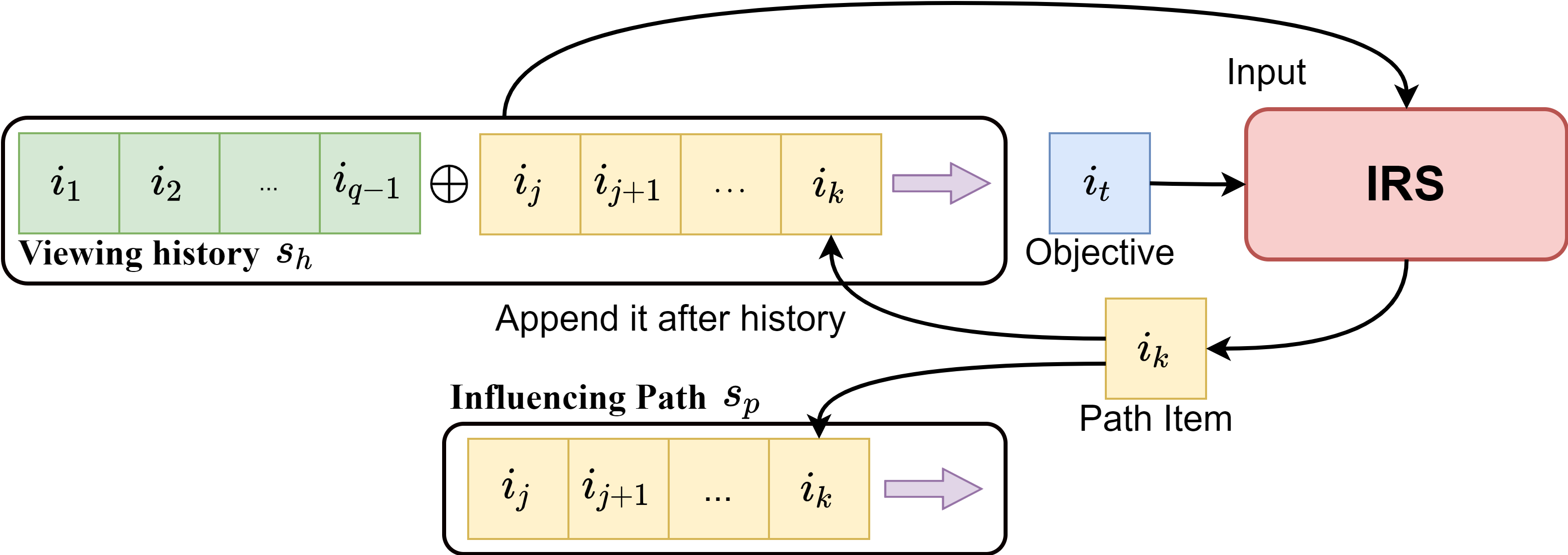
For simplicity, we assume that the user will passively accept any recommendation, and we employ probability measures to evaluate the user’s satisfaction with the influence path. Algorithm 1 demonstrates the overall workflow of IRS. The main goal of IRS is to learn the recommender function that progressively generates the influence path to lead the user towards the objective item and simultaneously satisfy the user’s interests. To achieve this goal, we present two baseline solutions adapted from existing URS and then our novel influential recommender model.
III-B Path-finding Algorithms as IRS
Given the problem setup of IRS, it is natural to consider the influence path generation process as a path-finding problem, namely, finding a path between two vertices on a graph that minimizes the cost. Since the original dataset is not a graph structure, we build an undirected graph from the user-item interaction sequences following the previous practice [33]. First, we map each item in the training dataset to a graph vertex. Then, we assign an edge to two vertices if the corresponding items appear consecutively in an interaction sequence and assign equal weight to each edge. For simplicity, we select the last item in the viewing history as the user’s recent interest and find a path between and the objective item using a path-finding algorithm such as Dijkstra. We name this framework as Pf2Inf.
Figure 3 illustrates an example of Pf2Inf. Given a new interaction history ending at and the objective item , Pf2Inf generates an influence path based on a shortest path algorithm.

III-C Adapting Existing RS with Greedy Search
Despite its simple architecture, Pf2Inf does not take into account the sequential patterns among items in the user’s viewing history. Neither does it work for sparse, disjoint graphs which are likely to exist in the sparse recommendation dataset. For example, in Figure 3, given the interaction history , it fails to find a reasonable path to the objective item by traversing the graph.
An alternative is to adapt an existing RS to IRS using a greedy search strategy. Specifically, we can generate an influence path with the following process: given user ’s viewing history , an existing RS can be used to generate the top- recommendations , which can then be re-sorted based on their distances to the objective item and the closest item is greedily selected into . The recommender repeats the process to generate the whole . The distance between two items can be calculated based on their embeddings (e.g. obtained from item2vec [12]). With this simple strategy, any existing RS can be adapted to generate the influence path, and we name this solution as Rec2Inf.
Depending on the backbone RS, the Rec2Inf framework can enable a recommender system to model user interests and sequential dependencies among items, and approach the objective item at the same time. However, it still suffers from the following limitations: (1) an item is greedily selected into the influence path in each step. The local optimal selections may not ultimately reach the global optimal influence path. For example, if the objective item deviates from the current user interests significantly and all candidate items in have large distances from , will have little effect in selecting the recommended items, hindering the influence path from reaching . (2) The objective item is not involved in the training process, which prevents the RS from planning early for reaching the goal of in the entire recommendation process.
III-D Influential Recommender Network (IRN)
To mitigate the challenges of the IRS framework, we propose Influential Recommender Network (IRN), a neural network model which progressively recommends items to persuade a user to approach the objective. IRN can learn the sequential patterns across item sequences, encode the characteristic of the objective item, and consider personalized impressionability at the same time. As shown in Figure 4, IRN is composed of three components: an embedding layer that vectorizes the input sequence, a stack of decoder layers, each of which comprises a self-attention layer with personalized masking, and an output layer that projects the hidden states of the decoder into probability distributions over items.

III-D1 Item Embedding
As items are originally represented as discrete tokens, we start by embedding them into dense vectors, which can be processed by deep neural networks. We convert items into both token and position embeddings, which, respectively, represent the context and the position of an item in the sequence. Given a sequence of items , we convert it to a sequence of -dimensional vectors , with each denoting the embedding for the j-th item, namely,
| (1) |
where denotes the token embedding matrix and denotes the positional encoding matrix, and ”+” refers to addition. Inspired by the well-known finding in NLP that better initial weights of token embedding can significantly improve the ultimate model performance [24], we use pre-trained embedding generated by the item2vec model [3].
III-D2 Decoder
A Transformer decoder takes the embedding sequence as input and sequentially generates items of the influence path based on the access history and the objective item. The decoder maintains a sequence of hidden states for the items in the sequence. The hidden state for item is computed based on the items before and the objective :
| (2) |
where denotes the hidden state of . The decoder consists of a stack of self-attention layers with each layer updating the hidden states based on the previous layer.
| (3) |
By stacking multiple decoder layers, the model is capable of learning more complicated patterns across the item sequence. In particular, the first decoder layer takes as input the embedding sequence as the initial hidden states: . Here, the self-attention layer performs the layer-wise transformation of the hidden states through the attention mechanism. It takes the hidden states as the input for query, key, and value to produce the aggregated value:
| (4) |
where denote the query, key, and value vectors, respectively. Specifically, we use multi-head attention, which is able to attend to information from different representation subspaces at different positions [22, 28, 20]. To enable the decoder to be aware of the objective item, we extend the self-attention layer with a Personalized Impressionability Mask (PIM). The PIM determines (1) which items can be seen by the attention layer, and (2) to what extent the item will be aggregated to produce the hidden states. We will discuss the two effects of PIM in the following sections.

III-D3 Perceiving objective
PIM is an extension of the standard attention mask in that it enables the decoder to perceive not only previous items but also the objective item. Figures 5(a) and 5(b) illustrate the idea. The standard Transformer decoder utilizes a causal (triangular) attention mask to prevent future items from participating in the prediction. Based on the causal attention, PIM introduces attention weights to the objective (Figure 5(b)). This enables the attention layer to be aware of the objective item in addition to the preceding items so that it can take in the extra effect of in generating the hidden states.
Furthermore, we propose a weighted attention mask to reflect the influence of the objective item (). As shown in Figure 5, each item in the input sequence corresponds to a mask weight (i.e. blue square), which will be added to calculate the attention weight inside the decoder. The item with a larger mask weight may contribute more since its corresponding attention weight is larger. Consequently, the item will be regarded as more relevant in generating the output. Let denote the mask weight for the objective item and denote the mask weight for the preceding history. We enforce the model to pay more attention to the objective item by setting . Additionally, by varying the scale of , we can control the aggressiveness degree of IRN in performing influential recommendations.
III-D4 Personalized Impressionability Factor
Users have personalized curiousness of exploration [46], which may affect their acceptance of external influence. For an impressionable user, IRN can be more aggressive and assign more weight to the objective, while for users who have focused interests, IRN should be less aggressive in approaching the objective and consider more the user’s historical interests. We define the Impressionability that measures the users’ acceptance of persuasion and utilize the Personalized Impressionability Factor, denoted by , to control the aggressiveness of influential recommendation. is integrated into the mask weight so that the self-attention model can have varying strategies for different users. is computed as:
| (5) | ||||
where denotes the embedding of with dimension , denotes the user embedding matrix, and denotes the parameters of the linear transformation. The factor is multiplied by the initial attention mask weight for the objective item , resulting in the final attention weights (Figure 5(c)). By integrating into the decoder, Equations 2 and 3 are extended as:
| (6) |
III-D5 Pre-padding Input Sequences
The original item sequences can have varying lengths. Therefore, to accommodate the PIM, we apply pre-padding on the input sequence instead of the widely used post-padding scheme [9]. For example, if the maximum sequence length is 5, then the pre-padded sequence for is , while the post-padded sequence is , where is the padding token. Pre-padding allows the objective item to stay at a fixed position (i.e., the last item in the sequence) whereas post-padding has different positions for the objective item depending on the sequence length. The fixed position of the objective item avoids extra noise brought to the model due to the variable-length input sequences in position encoding and accelerates the computation [21].
III-D6 Output Probability
Finally, we project the decoder output to the item space with a linear layer and generate the output probability using the softmax function. Formally, the probability distribution for generating the -th item can be computed as:
| (7) |
where is the projection matrix. IRN recommends an influence path by generating items one by one according to the probability distribution at each step.
III-D7 Objective Function
Given a sequence of items for user (), where the last item is selected as the objective item (). Assuming that ’s interests start at , the actual path from to should have maximized probability, which is equivalent to minimizing the conditional perplexity:
| (8) | ||||
Apart from items preceding in the sequence, the conditional probability of considers both the objective item and the personalization of . To avoid numerical underflow, we minimize its logarithmic form instead, which is equivalent to minimizing the cross-entropy loss function:
| (9) |
where . It is worth noting that each sequence belongs to one user and one user may have multiple sequences.
IV Experiment
We evaluate the proposed framework using two commonly used recommendation datasets. To meet the requirement of IRS, we design several new metrics to assess the model performance. Since IRS recommends an item sequence, many sequence-item interactions may not exist in the original dataset, making it difficult to evaluate the user’s acceptance of these items. To mitigate the problem, we use a trained evaluator to provide probability measures for the unknown sequence-item interactions. We will explain in detail the experiment design and outcomes in the remaining sections.
| Dataset | Users | Items | Interactions | Density | Avg. Items |
|---|---|---|---|---|---|
| per User | |||||
| Lastfm | 896 | 2,682 | 28,220 | 1.17% | 31 |
| Movielens-1m | 6,040 | 3,415 | 996,183 | 4.83% | 164 |
IV-A Datasets
Since online user-item interaction datasets with feedback from real users are not available, we design experiments based on offline datasets that are suitable for the influential recommendation. Specifically, we consider datasets that satisfy the following properties : (1) user-item interactions should exhibit sequential patterns and interaction timestamps are available, and (2) cost in user-item interactions should not be too high to be practical. For example, e-commerce purchase datasets may not be suitable because promoting the objective item by asking the user to buy other items is less practical. Taking these requirements into consideration, we select two widely used datasets, namely, Movielens-1m11 1 https://grouplens.org/datasets/movielens/1m and Lastfm22 2 https://grouplens.org/datasets/hetrec-2011/ which have timestamps indicating when the user-item interactions take place. Moreover, watching movies and listening to music have relatively low costs.
IV-A1 Preprocessing
Following the common practice [11, 40], we consider all numeric ratings (tagging behavior) as positive feedback. For both datasets, we group the interaction records by the user and order the sequence by interaction timestamps. For the Lastfm dataset, we combine multiple consecutive behaviors of the same user-item pair into one single interaction. To better reveal the sequential patterns encoded in the dataset, we follow the common practice [26, 20, 45, 28] and filter out users and items with less than interactions. Table I shows the statistics of the final dataset.
IV-A2 Dataset Splitting
We split the dataset into training and testing sets through the following steps. Given a user ’s complete viewing history , we retain the last item for the next-item evaluation task in testing and randomly split the remaining part into multiple continuous, non-overlapping subsequences , where each subsequence’s length is between and . For viewing history that is shorter than , we prolong its length to through padding. We set , for Lastfm and , for Movielens-1m, respectively. The last item of each subsequence is selected as the objective item during the training of IRN. All subsequences of a user constitute the user’s sequence set , and the model training and validation are based on . To construct the testing set, we obtain the starting user behavior sequence for each user. Based on the and an objective item , each IRS framework generates the influence path following the process illustrated in Figure 2. We will further explain the criteria for choosing in Section IV-B1. Finally, we obtain a testing set of size . It is worth noting that the test set does not contain ground-truth paths and each IRS model generates influence paths based on the same test set independently.
IV-B IRS Evaluation
IV-B1 Objective Item Selection
As introduced in previous sections, the objective item can influence the IRS’s strategy when generating the influence path . For the sake of fairness, for each in the testing set, we randomly sample an objective item from the whole item space based on the following criteria: (1) . Under the problem formulation of IRS, the objective should be a new item to the user. (2) has at least interaction records. This prevents unpopular items from being selected as the objective item.
IV-B2 Evaluation Metrics
Different from the traditional “next-item” RS which only needs to evaluate the single recommended item based on a user’s viewing history, IRS has to evaluate the influence path (i.e., a sequence of recommended items), where both the user acceptance and the path’s smoothness need to be taken into account. For example, a long influence path may turn out to be continuously related to the user’s current interest but fail to reach the objective item, while a short influence path may recommend the objective item directly but deviates too much from the user’s interest and is therefore rejected by the user.
In order to measure a user’s interest over the influence path , or whether can better lead the user towards the objective item , we need to estimate the joint probability as well as the conditional probability . This can be formulated as a language model which defines the probability of each sequence appearing in a sequence corpora:
| (10) |
For these concerns, we evaluate the influence path from two aspects: (1) whether the influence path can successfully shift the user interests towards the objective , and (2) whether satisfies the user’s interest. We design and employ the following metrics:
- •
Success Rate () measures the ratio of generated ’s that can successfully reach the objective item within the maximum length (as denoted in Algorithm 1):
(11) - •
Increase of Interest () measures the change of user’s interest in the objective item after being persuaded through :
(12) where “” refers to the concatenation of two sequences; is the probability that the objected item is accepted by a user with viewing sequence . Here we use log form probability to avoid numerical underflow.
- •
Increment of Rank () measures the increase of the ranking for the objective item after being persuaded through :
(13) where denotes the ranking of the objective item based on .
- •
Perplexity (PPL) measures the naturalness and smoothness of the influence path , that is, how likely the path can appear in the viewing history. In our experiment, PPL is defined as the conditional probability of that follows :
(14) where denotes the concatenated sequence of the viewing history and the preceding items of in , and denotes the length of . Note that the logarithm form of perplexity is equivalent to the average of the log probability that the user accepts the path item in each step of the influence path.
IV-B3 IRS Evaluator
As introduced above, the computation of , , and PPL relies on the term , which refers to the probability that item is accepted by a user given the viewing history . This presents a unique challenge for the offline evaluation of IRS with the logged dataset: many sequence-item interactions may not exist in the users’ viewing histories, especially when the sequence is long.
Traditional NLP approaches estimate the term by counting the occurrences of items as follows:
| (15) |
where refers to the times that sequence occurs in the sequence corpora and refers to the new sequence with appended into . Due to the sparsity of RS datasets, there can be many zero counts (i.e., ) in computing the conditional probabilities, which makes the counting approximation approach ineffective.
Inspired by the common practice of simulation based experiments in reinforcement learning based RS [8, 15, 23, 16] and combinatorial recommendation [44, 32], we adopt an independent IRS evaluator to tackle the problem. The evaluator measures the relevance of item by estimating the probability of item following the sequence , namely,
| (16) |
Specifically, we train an independent next-item recommender model which outputs a measurement for the probability term . The recommender model contains a softmax layer which generates a probability distribution over all items given an input sequence . Finally, we compute as:
| (17) | ||||
Although the evaluator is an approximation of real users, it provides a reasonably fair offline evaluation strategy for sequence-item interactions that do not appear in the dataset.
An accurate evaluator should be capable of capturing the sequential patterns encoded in the viewing sequence and recommend the next item accurately. Therefore, we experiment with multiple state-of-the-art sequential recommenders and select the optimal one as the final evaluator. We measure the performance of the evaluator using HR@20 (Hit Ratio) and MRR (Mean Reciprocal Rank):
| (18) | ||||
where denotes the size of the testing set, the viewing history sequence (not containing ) of user , and the ranking of item in each IRS; equals to if the condition “” is true and otherwise. Recall that the last item () of the input sequence is the labelled item.
Specifically, we consider the following models for the IRS evaluator:
- •
GRU4Rec [13] employs the recurrent neural network (RNN) based architecture to model user behavior sequences for sequential recommendation.
- •
Caser [30] utilizes the convolutional neural network (CNN) to learn the sequential patterns of user-item interactions in both horizontal and vertical way.
- •
SASRec [20] models the sequential dynamics of recommendation by using a self-attention-based model, which allows for capturing both long-term and short-term semantics.
- •
Bert4Rec [28] further improves the user behavior sequences modeling with bidirectional self-attention and is considered one of the strongest baselines for the sequential recommendation.
The original models were implemented in various deep learning frameworks, and we port them to PyTorch based on the originally published code33 3 https://github.com/graytowne/caser_pytorch44 4 https://github.com/hidasib/GRU4Rec55 5 https://github.com/kang205/SASRec66 6 https://github.com/FeiSun/BERT4Rec. We tune all hyperparameters of these models using the validation set and compare their results on the testing set.
| Lastfm | Movielens-1M | |||
|---|---|---|---|---|
| Method | ||||
| GRU4Rec | 0.0392 | 0.0081 | 0.243 | 0.063 |
| Caser | 0.0460 | 0.0106 | 0.252 | 0.062 |
| SASRec | 0.0445 | 0.0097 | 0.257 | 0.062 |
| Bert4Rec | 0.0489 | 0.0199 | 0.264 | 0.076 |
Table II shows the comparison results of IRS evaluators. Among the tested sequential recommender models, Bert4Rec has achieved the best performance in terms of all evaluation metrics, with around and improvements against the second-best model. Therefore, Bert4Rec is selected as the evaluator and used to provide a probability measure of in the following experiment discussion.
| Lastfm | Movielens-1M | ||||||||
| (PPL) | (PPL) | ||||||||
| Pf2Inf | Dijkstra | 0.031 | 0.0192 | 3.73 | 9.88 | 0.069 | 0.009 | 362.8 | 6.97 |
| MST | 0.0016 | -0.0531 | -11.5 | 8.13 | 0.031 | -0.026 | 52.0 | 8.47 | |
| Vanilla | POP | 0.00 | -0.0119 | 9.74 | 7.27 | 0.005 | -0.078 | 18.1 | 5.39 |
| BPR | 0.001 | -0.123 | 5.57 | 6.64 | 0.006 | -0.171 | 41.5 | 5.62 | |
| TransRec | 0.00 | -0.0720 | -0.483 | 6.69 | 0.005 | 0.083 | 19.9 | 5.11 | |
| GRU4Rec | 0.001 | -0.0818 | 4.72 | 6.27 | 0.00 | -0.583 | -7.32 | 4.41 | |
| Caser | 0.002 | 0.0110 | 13.6 | 6.71 | 0.00 | -0.887 | 7.36 | 3.78 | |
| SASRec | 0.00 | 0.0257 | -15.0 | 6.36 | 0.001 | -0.003 | -0.918 | 3.95 | |
| Rec2Inf | POP | 0.0234 | 0.203 | 47.7 | 7.46 | 0.019 | 1.35 | 238.9 | 5.89 |
| BPR | 0.0279 | -0.0218 | 41.9 | 6.80 | 0.021 | 0.930 | 242.8 | 6.01 | |
| TransRec | 0.0625 | 0.0218 | 48.9 | 6.77 | 0.042 | 1.59 | 508.0 | 5.50 | |
| GRU4Rec | 0.0140 | 0.0392 | 20.8 | 6.37 | 0.012 | 0.91 | 130.1 | 5.22 | |
| Caser | 0.0246 | 0.0236 | 15.82 | 6.81 | 0.073 | 1.38 | 614.0 | 4.74 | |
| SASRec | 0.0137 | 0.0205 | 42.7 | 7.78 | 0.014 | 1.10 | 139.8 | 6.03 | |
| IRN | 0.142 | 0.572 | 160.7 | 6.65 | 0.259 | 2.61 | 804.7 | 4.94 | |
IV-C Baselines
We compare our approach with two path-finding algorithms under the Pf2Inf framework and six RS baselines under the Rec2Inf framework. Overall, we use the following approaches as baselines:
- •
Dijkstra finds the shortest path between two nodes in the item graph (described in Section III-B). We select the influence path as the first items along the path from the last item in to .
- •
MST constructs a minimum spanning tree from the constructed item graph. We select the influence path using the same process as Dijkstra.
- •
POP sorts all the items by occurrence and recommends the most popular items to the user.
- •
BPR [25] is a commonly used matrix factorization method that optimizes a pairwise objective function.
- •
TransRec [10] models item-item and user-item translation relationships for large-scale sequential prediction.
- •
GRU4Rec [13] is an RNN based model for sequential recommendation.
- •
Caser [30] is a CNN based model for sequential recommendation.
- •
SASRec [20] is a sequential recommender based on self-attention.
For RS approaches under the Rec2Inf framework, we use the recommended hyperparameters in the original implementation and set the size of the candidate set . We calculate the item distance using genre feature vector on Movielens-1m, and item2vec [3] embeddings on Lastfm, respectively.
IV-D Experiment Result
IV-D1 Overall Comparison
Table III shows the overall results of various models on the two datasets. As we can see, IRN significantly outperforms other baselines in terms of , , and on both datasets. In the Lastfm dataset, of the influence paths generated by IRN for the testing set can reach the objective item within steps. In the Movielens-1M dataset, of testing sequences can successfully lead to the objective item, while the strong baseline method Caser can only achieve 7.3%. In terms of PPL, IRN achieves the second best results, only next to TransRec in Lastfm and Caser in Movielens-1m, respectively. It indicates that IRN does not hamper the smoothness of the influence path while achieving superior influencing performance. Note that a trade-off exists between the influencing power of the recommender and the smoothness of the influence path. We will further discuss the aggressiveness of IRS in Section IV-D3.
In comparison, Dijkstra under the Pf2Inf framework achieves greater influencing performance at the cost of high PPL. This indicates that although path-finding algorithms manage to find a path from the viewing history to the objective, it often fails to satisfy the user’s current interests and is likely to be rejected by users in the middle of persuasion. We also compare IRN with the vanilla versions (i.e., the original model without being adapted to the Rec2Inf paradigm) of baselines. The influence path of each vanilla model is generated by repeatedly recommending the item with the maximum . Since the vanilla model is driven solely by users’ current interest, we can observe a and approximately equal to zero for most vanilla baselines. Compared to their vanilla versions, these adapted baselines can achieve a higher and have a significantly larger and , which indicates that the Rec2Inf frameworks are effective in increasing the user’s interest in the objective item. However, the adapted baselines generally have a higher PPL. It is reasonable because they need to pay extra attention to the objective item at each step of the influence path, frequently resulting in a recommendation that suits the user’s interest less.
In summary, IRN outperforms the baselines in most evaluation metrics, which validates its capability of generating natural and smooth influence paths.
IV-D2 Short-term Interests Match
In addition to evaluating the influencing power of the recommender models, we also investigate whether they can achieve comparable performance in the task of traditional next-item recommendation.
Table IV displays the performance of various models in terms of next-item recommendation. In general, baseline models under the IRS framework achieve suboptimal performance compared to the state-of-the-art next-item recommenders. We also observe a performance loss compared to their vanilla versions under the Rec2Inf framework. The reason could be that the IRS needs to shift towards the objective early if is far from the user’s current interest. This cause the model to recommend an unfamiliar item to the user, thus reducing the recommendation accuracy. Yet IRN achieves comparable results with respect to and on the two datasets, with around and performance loss compared to the best-performed . This indicates that even with the objective item , IRN can still capture the user’s current interests without abruptly heading for .
| Lastfm | Movielens-1M | |||||
| GRU4Rec | 0.0392 | 0.0081 | 0.243 | 0.063 | ||
| Next-item | Caser | 0.0460 | 0.0106 | 0.252 | 0.062 | |
| RS | SASRec | 0.0445 | 0.0097 | 0.257 | 0.062 | |
| Bert4Rec | 0.0489 | 0.0199 | 0.264 | 0.081 | ||
| IRS | GRU4Rec | 0.0387 | 0.0079 | 0.198 | 0.047 | |
| Caser | 0.0430 | 0.0102 | 0.250 | 0.061 | ||
| SASRec | 0.0437 | 0.0092 | 0.207 | 0.041 | ||
| IRN | 0.0458 | 0.0190 | 0.242 | 0.073 | ||

IV-D3 Aggressiveness of IRS
One notable phenomenon observed in Section IV-D1 is that even though IRN significantly outperforms the baselines, the majority of the generated influence paths cannot successfully end at the objective item (e.g., is only 14.2% and 25.9% on the two datasets, respectively). In this section, we study this phenomenon by analyzing the aggressiveness of influence paths. We hypothesize that whether can reach the objective item is mainly influenced by two factors: the maximum path length and the Aggressiveness Degree (AD) of each IRS. Hence, we investigate the relation between these two factors and the success rate of reaching the objective item ().
Figure 6 illustrates the relationship between the maximum path length and the success rate. For clarity, we only compare IRN to the strong baselines in the Rec2Inf framework. In general, for all methods, the success rate increases as increases since longer influence paths increase the chance of reaching the objective. In addition to the outstanding performance, IRN achieves a steady improvement of as the influence path length increases, whereas the baselines’ quickly flattens out to a low level. This can be attributed to the fact that IRN incorporates the objective item in the training process, thus enabling long-range planning in the influencing process. In contrast, the baseline models make an influential recommendation at each step independently and locally.
Figure 7 illustrates the impact of aggressiveness degree (AD) when IRS is approaching the objective item. Each recommender has its own parameters to control the AD. As we can see, AD for the baselines is correlated to the size of the candidate set . As introduced in Section III-C, the Rec2Inf framework selects the item that is closest to the objective from the top candidate set. When , this is equivalent to the original recommender system which simply predicts the next item without considering the objective. When is set to the total number of items, it may recommend the objective item directly which has zero distance to itself. Different from the baselines, AD for IRN is related to the objective mask weight . Larger enforces the model to rely more on the objective item in the recommendation.
In order to compare AD’s influence to baselines and IRN, we need to unify AD’s of different methods to the same scale. Therefore, we set 5 levels of for Rec2Inf baselines and 5 levels of for IRN, both 5 levels are then mapped as the x-axis of Figure 7. Figures 7(a) and (b) show the value of under different levels of ADs. As expected, when AD increases, increases accordingly since more attention on the objective item can increase the chance of reaching the objective. In addition, IRN significantly outperforms the baselines given the same AD. This indicates that the model is effective in leading users towards the objective. Figures 7(c) and (d) depict the perplexity over different levels of ADs. A higher perplexity indicates a lower likelihood that users accept the influence paths. As we can see, most baseline methods exhibit a clear trade-off between and PPL (higher tends to have low PPL), probably because the aggressive influencing strategy increases the abruptness of sequential recommendation. In contrast, IRN is superior to other models with a significantly higher and a smaller PPL, demonstrating its capability of effectively leading users towards the objective and maintaining a high level of smoothness. Furthermore, we observe that there does not exist a universal optimal AD which can achieve the best and PPL simultaneously. This indicates that the selection of AD in the IRS framework should be adapted to the requirement of the applications.

IV-D4 Effectiveness of the Personalized Mask Weight

| Mask Type | Lastfm | Movielens-1M | ||||
|---|---|---|---|---|---|---|
| Type 1 | 5.93 | 0.002 | 0.011 | 4.27 | 0.009 | 0.054 |
| Type 2 | 6.55 | 0.118 | 0.477 | 4.92 | 0.232 | 2.01 |
| Type 3 | 6.65 | 0.142 | 0.572 | 4.94 | 0.259 | 2.61 |
As introduced in Section III-D, The Personalized Impressionability Mask (PIM) models a user’s personal impressionability about the persuasion. Table V compares the performance of various masking schemes. In “Type 1” the model will not pay extra attention to the objective (i.e., ), in “Type 2” the objective has a uniform large weight (), and in “Type 3” the model integrates the Personalized Impressionability Factor and the objective has weight . Compared to “Type 1”, “Type 2” has significantly improved the user’s acceptance of the objective item (measured by and ) at the expense of the smoothness of the path (measured by ). The addition of further increases the influence performance by approximately without evident impact to the smoothness.
The IRN learns for each user. We further investigate the distribution over values, as shown in Figure 8. A larger indicates that the user is more adventurous and prefers a larger AD. Thus, recommended items by IRN are more close to the objective. On the other hand, a smaller results in recommendations that depend more on the user’s historical interests. In general, follows a normal distribution on both datasets. This validates our intuition that users are indeed different in accepting influential recommendations and that PIM is effective in modeling their different personalities.
IV-D5 Stepwise evolution of User Interests
To get a deeper insight into the influencing process, we study the evolution of the influence path in each step. This gives us a micro view of how IRS leads the user towards the objective. Specifically, we analyze two probabilities, namely, the “objective probability” (i.e., the probability that the user likes objective item at the influencing step) and “item probability” (i.e., the probability that the user is satisfied with item at the influencing step) over all the influence paths, which can be calculated using the IRS evaluator . To facilitate analysis, we average the two probabilities on the testing sequences. Note that influence paths may have various lengths due to early reach to the objective, which affects the averaging of and . Therefore, we exclude early-success paths which account for only a small fraction given .
Figure 9 presents the results of stepwise user interests evolution. On both datasets, the influence paths generated by IRN can lead the user towards the objective steadily while maintaining a high probability to be accepted by the user. In comparison, influence paths recommended by most adapted baselines cannot steadily lead users to the objective, as evident from their flat curves. In the Movielens-1m dataset, the suboptimal approach Caser also demonstrates a steadily increasing probability curve of the user accepting the objective item, but the increase amplitude is far below IRN. Experiment results show that IRN can consistently utilize the sequential dependence signals accumulated throughout the evolution of the influence path.

IV-D6 Hyperparameter Tuning and Ablation Study
We run IRN with different combinations of hyperparameter settings and find the optimal group of parameters using grid search. We optimize IRN using the Adam algorithm with a dynamic learning rate scheduler which reduces the learning rate by a factor of once the learning stagnates.
The ranges and optimal values of the hyperparameters are shown in Table VI. and refer to the minimum and maximum sequence lengths related to the dataset splitting as introduced in Section IV-A2. denotes the starting learning rate for the model which ranges from to . denotes the embedding size of items, while denotes the embedding size of users. denotes the number of decoder layers, denotes the number of heads for attention, and is related to the weight of the attention mask for the objective item. With the optimal setting of hyperparameters, the training of IRN takes approximately 1 hour on Lastfm and 2 hours on Movielens-1M, respectively, using a machine with one GTX-2080Ti GPU. In terms of scalability, the computational perplexity of IRN is where and refer to the input length and the item set, respectively. The framework can be easily paralleled to multiple GPUs to accelerate the computation without significantly affecting the performance.
| Name | Range | Lastfm | Movielens-1m |
| [30, 40, 50, 60, 70, 80] | 50 | 60 | |
| - | 20 | 20 | |
| Batch size | {64, 128, 256, 512} | 128 | 128 |
| [1e-4, 1e-2] | 8e-3 | 3e-3 | |
| {10, 20, 30, 40} | 40 | 30 | |
| {4, 6, 8, 10,12} | 10 | 10 | |
| {4, 5, 6, 7, 8} | 5 | 6 | |
| {0, 0.25, 0.5, 0.75, 1} | 1 | 1 | |
| {1, 2, 3, 4, 5, 6, 7, 8} | 4 | 6 |
IV-D7 Case Study
In addition to the quantitative studies, we demonstrate the effectiveness of IRN with a real case. We provide a real influence path generated by IRN from the Movielens dataset. As is shown in Table VII, the Mille bolle blu with a genre of “Comedy” was selected as the objective item while the user’s viewing history ends at Bulletproof with a genre of “Action”. In the initial few steps, IRN recommended movies in “Action”, “Adventure”, and “Thriller”. After a few swinging attempts between “Adventure” and “Thriller”, the Space Jam with genres “Adventure”, “Children”, and “Comedy” was recommended, followed by First Kid with genres “Children” and “Comedy”. The last few movies are classified into “Comedy”. From the example, we can observe a smooth genre transition from “Action” to “Comedy”. The results affirm the effectiveness of IRN in leading the user towards the objective item smoothly.
| Name | Genre |
|---|---|
| The last movie in the viewing history: | |
| Bulletproof (1996) | Action |
| The movies in the influence path: | |
| Lost World: Jurassic Park (1997) | Action, Adventure, Sci-Fi, Thriller |
| Chain Reaction (1996) | Action, Adventure, Thriller |
| Anaconda (1997) | Action, Adventure, Thriller |
| Broken Arrow (1996) | Action, Thriller |
| Fled (1996) | Action, Adventure |
| Glimmer Man (1996) | Action, Thriller |
| Space Jam (1996) | Adventure, Animation, Children, |
| Comedy, Fantasy | |
| First Kid (1996) | Children, Comedy |
| Jack (1996) | Comedy, Drama |
| Michael (1996) | Comedy, Romance |
| Mille bolle blu (1993)* | Comedy |
V Conclusion
We introduce a new recommendation paradigm termed Influential Recommender System (IRS), which proactively and incrementally expands a user’s interest toward an objective item by recommending to the user a sequence of items. We design a Transformer-based sequential model Influential Recommender Network (IRN) with Personalized Impressionability Mask (PIM) to model, respectively, the sequential dependencies among the items and individual users’ personalized acceptance of external influence. Evaluation metrics are carefully designed for the influential recommendation task. Experimental results show that IRN significantly outperforms the baseline recommenders and demonstrate IRN’s capability in smooth and progressive persuasion.
Since this is the first work that proposes the idea of influential recommendation, we are in the exploratory stage for this new recommendation problem. Many issues remain to be further studied. We summarize the future work in the following directions. (1) Extend the path-finding baseline by incorporating knowledge graphs (KG). Knowledge graphs have been extensively used in recommendation systems, making them a natural fit of the IRS framework. For example, we can model the user’s historical interests as a subgraph and expand the subgraph toward the objective item. (2) Improve the evaluation of unknown sequence-item interactions. Due to the limitation of the offline dataset used in this work, we utilize an evaluator to stimulate the user’s interest in a new incoming item, which may incur bias in calculating the IRS evaluation metrics. A better solution is to deploy the IRS in an online recommendation platform where honest user feedback is available or to conduct a human experiment to evaluate the generated influence paths. (3) Expand the scope of the objective in IRS. In this work, the proposed framework aims at leading the user to like a single objective item, which naturally leads to a broader problem setting where the objective can be a collection of items, a category, a topic, etc. (4) Consider the stepwise dynamics in generating the influence path. For simplicity, we assume that the user passively accepts the recommended items and evaluates the influence path as a whole. However, in a more practical application scenario, it is important to consider the stepwise user response to a recommended item in approaching the objective. For example, a user may reject an intermediate item in a pre-scheduled influence path, and the IRS needs to alter its strategy by recommending another item to persuade the user towards the objective.
Acknowledgment
The authors would thank anonymous reviewers for their valuable comments and suggestions. This work was sponsored by Research Grants Council HKSAR GRF (No. 16215019), NSFC (No. 62102244), CCF-Tencent Open Research Fund (RAGR20220129), and Guang Dong Innovative Yong Talents Program (No. R5201919).
References
- [1] I. Ajzen. Attitudes and persuasion. 2012.
- [2] I. Arieli and Y. Babichenko. Private bayesian persuasion. Journal of Economic Theory, 182:185–217, 2019.
- [3] O. Barkan and N. Koenigstein. Item2vec: neural item embedding for collaborative filtering. In 2016 IEEE 26th International Workshop on Machine Learning for Signal Processing (MLSP), pages 1–6. IEEE, 2016.
- [4] D. Bergemann and S. Morris. Information design, bayesian persuasion, and bayes correlated equilibrium. American Economic Review, 106(5):586–91, 2016.
- [5] H. Bharadhwaj, H. Park, and B. Y. Lim. Recgan: recurrent generative adversarial networks for recommendation systems. In Proceedings of the 12th ACM Conference on Recommender Systems, pages 372–376, 2018.
- [6] S. Chaiken. The heuristic model of persuasion. In Social influence: the ontario symposium, volume 5, pages 3–39, 1987.
- [7] Y.-K. Che and J. Hörner. Recommender systems as mechanisms for social learning. The Quarterly Journal of Economics, 133(2):871–925, 2018.
- [8] M. Chen, A. Beutel, P. Covington, S. Jain, F. Belletti, and E. H. Chi. Top-k off-policy correction for a reinforce recommender system. In Proceedings of the Twelfth ACM International Conference on Web Search and Data Mining, pages 456–464, 2019.
- [9] M. Dwarampudi and N. Reddy. Effects of padding on lstms and cnns. arXiv preprint arXiv:1903.07288, 2019.
- [10] R. He, W.-C. Kang, and J. McAuley. Translation-based recommendation. In Proceedings of the eleventh ACM conference on recommender systems, pages 161–169, 2017.
- [11] R. He and J. McAuley. Fusing similarity models with markov chains for sparse sequential recommendation. In 2016 IEEE 16th International Conference on Data Mining (ICDM), pages 191–200. IEEE, 2016.
- [12] X. He, L. Liao, H. Zhang, L. Nie, X. Hu, and T.-S. Chua. Neural collaborative filtering. In Proceedings of the 26th international conference on world wide web, pages 173–182, 2017.
- [13] B. Hidasi and A. Karatzoglou. Recurrent neural networks with top-k gains for session-based recommendations. In Proceedings of the 27th ACM international conference on information and knowledge management, pages 843–852, 2018.
- [14] B. Hidasi, A. Karatzoglou, L. Baltrunas, and D. Tikk. Session-based recommendations with recurrent neural networks. arXiv preprint arXiv:1511.06939, 2015.
- [15] J. Huang, H. Oosterhuis, M. de Rijke, and H. van Hoof. Keeping Dataset Biases out of the Simulation: A Debiased Simulator for Reinforcement Learning Based Recommender Systems, page 190–199. 2020.
- [16] J. Huang, H. Oosterhuis, M. de Rijke, and H. van Hoof. Keeping dataset biases out of the simulation: A debiased simulator for reinforcement learning based recommender systems. In Fourteenth ACM Conference on Recommender Systems, pages 190–199, 2020.
- [17] A. Jadbabaie, P. Molavi, A. Sandroni, and A. Tahbaz-Salehi. Non-bayesian social learning. Games and Economic Behavior, 76(1):210–225, 2012.
- [18] E. Kamenica. Bayesian persuasion and information design. Annual Review of Economics, 11:249–272, 2019.
- [19] E. Kamenica and M. Gentzkow. Bayesian persuasion. American Economic Review, 101(6):2590–2615, 2011.
- [20] W.-C. Kang and J. McAuley. Self-attentive sequential recommendation. In 2018 IEEE International Conference on Data Mining (ICDM), pages 197–206. IEEE, 2018.
- [21] G. Li, Y. Xi, J. Ding, D. Wang, B. Liu, C. Fan, X. Mao, and Z. Zhao. Easy and efficient transformer: Scalable inference solution for large nlp model. arXiv preprint arXiv:2104.12470, 2021.
- [22] J. Li, Z. Tu, B. Yang, M. R. Lyu, and T. Zhang. Multi-head attention with disagreement regularization. arXiv preprint arXiv:1810.10183, 2018.
- [23] L. Li, S. Chen, J. Kleban, and A. Gupta. Counterfactual estimation and optimization of click metrics in search engines: A case study. In Proceedings of the 24th International Conference on World Wide Web, pages 929–934, 2015.
- [24] X. Qiu, T. Sun, Y. Xu, Y. Shao, N. Dai, and X. Huang. Pre-trained models for natural language processing: A survey. Science China Technological Sciences, pages 1–26, 2020.
- [25] S. Rendle, C. Freudenthaler, Z. Gantner, and L. Schmidt-Thieme. Bpr: Bayesian personalized ranking from implicit feedback. arXiv preprint arXiv:1205.2618, 2012.
- [26] S. Rendle, C. Freudenthaler, and L. Schmidt-Thieme. Factorizing personalized markov chains for next-basket recommendation. In Proceedings of the 19th international conference on World wide web, pages 811–820, 2010.
- [27] G. Romanyuk and A. Smolin. Cream skimming and information design in matching markets. American Economic Journal: Microeconomics, 11(2):250–76, 2019.
- [28] F. Sun, J. Liu, J. Wu, C. Pei, X. Lin, W. Ou, and P. Jiang. Bert4rec: Sequential recommendation with bidirectional encoder representations from transformer. In Proceedings of the 28th ACM international conference on information and knowledge management, pages 1441–1450, 2019.
- [29] J. Tang, F. Belletti, S. Jain, M. Chen, A. Beutel, C. Xu, and E. H. Chi. Towards neural mixture recommender for long range dependent user sequences. The World Wide Web Conference on - WWW ’19, 2019.
- [30] J. Tang and K. Wang. Personalized top-n sequential recommendation via convolutional sequence embedding, 2018.
- [31] A. Vaswani, N. Shazeer, N. Parmar, J. Uszkoreit, L. Jones, A. N. Gomez, Ł. Kaiser, and I. Polosukhin. Attention is all you need. In Advances in neural information processing systems, pages 5998–6008, 2017.
- [32] F. Wang, X. Fang, L. Liu, Y. Chen, J. Tao, Z. Peng, C. Jin, and H. Tian. Sequential evaluation and generation framework for combinatorial recommender system. arXiv preprint arXiv:1902.00245, 2019.
- [33] J. Wang, P. Huang, H. Zhao, Z. Zhang, B. Zhao, and D. L. Lee. Billion-scale commodity embedding for e-commerce recommendation in alibaba. In Proceedings of the 24th ACM SIGKDD International Conference on Knowledge Discovery & Data Mining, pages 839–848, 2018.
- [34] S. Wang, L. Hu, L. Cao, X. Huang, D. Lian, and W. Liu. Attention-based transactional context embedding for next-item recommendation. 2018.
- [35] S. Wang, L. Hu, Y. Wang, L. Cao, Q. Z. Sheng, and M. Orgun. Sequential recommender systems: Challenges, progress and prospects. In Proceedings of the Twenty-Eighth International Joint Conference on Artificial Intelligence, IJCAI-19, pages 6332–6338, 7 2019.
- [36] S. Wang, L. Hu, Y. Wang, Q. Z. Sheng, M. Orgun, and L. Cao. Modeling multi-purpose sessions for next-item recommendations via mixture-channel purpose routing networks. In Proceedings of the Twenty-Eighth International Joint Conference on Artificial Intelligence, IJCAI-19, pages 3771–3777. International Joint Conferences on Artificial Intelligence Organization, 7 2019.
- [37] Z. Wang, W. Wei, G. Cong, X.-L. Li, X.-L. Mao, and M. Qiu. Global context enhanced graph neural networks for session-based recommendation. In Proceedings of the 43rd International ACM SIGIR Conference on Research and Development in Information Retrieval, pages 169–178, 2020.
- [38] C.-Y. Wu, A. Ahmed, A. Beutel, A. J. Smola, and H. Jing. Recurrent recommender networks. WSDM ’17, pages 495–503. ACM, 2017.
- [39] S. Wu, Y. Tang, Y. Zhu, L. Wang, X. Xie, and T. Tan. Session-based recommendation with graph neural networks. In Proceedings of the AAAI conference on artificial intelligence, volume 33, pages 346–353, 2019.
- [40] Y. Wu, C. DuBois, A. X. Zheng, and M. Ester. Collaborative denoising auto-encoders for top-n recommender systems. In Proceedings of the Ninth ACM International Conference on Web Search and Data Mining, pages 153–162, 2016.
- [41] L. Xiang, Q. Yuan, S. Zhao, L. Chen, X. Zhang, Q. Yang, and J. Sun. Temporal recommendation on graphs via long-and short-term preference fusion. In Proceedings of the 16th ACM SIGKDD international conference on Knowledge discovery and data mining, pages 723–732, 2010.
- [42] H. Ying, F. Zhuang, F. Zhang, Y. Liu, G. Xu, X. Xie, H. Xiong, and J. Wu. Sequential recommender system based on hierarchical attention network. In Proceedings of the 27th International Joint Conference on Artificial Intelligence, IJCAI’18, page 3926–3932. AAAI Press, 2018.
- [43] F. Yuan, A. Karatzoglou, I. Arapakis, J. M. Jose, and X. He. A simple convolutional generative network for next item recommendation. WSDM ’19, page 582–590, 2019.
- [44] Y. Yue and C. Guestrin. Linear submodular bandits and their application to diversified retrieval. Neural Information Processing Systems, 2011.
- [45] T. Zhang, P. Zhao, Y. Liu, V. S. Sheng, J. Xu, D. Wang, G. Liu, and X. Zhou. Feature-level deeper self-attention network for sequential recommendation. In IJCAI, pages 4320–4326, 2019.
- [46] P. Zhao and D. L. Lee. How much novelty is relevant? it depends on your curiosity. In Proceedings of the 39th International ACM SIGIR conference on Research and Development in Information Retrieval, pages 315–324, 2016.