Stellar Rotation and Structure of the Persei Complex
When Does Gyrochronology Start to Work?Facilities: TESS (Ricker et al. 2015), Gaia (Gaia Collaboration et al. 2016; Gaia Collaboration et al. 2022), LAMOST (Cui et al. 2012)
Astropy (Astropy Collaboration et al. 2013; Astropy Collaboration et al. 2018; Astropy Collaboration et al. 2022), astrobase (Bhatti et al. 2017), Matplotlib (Hunter 2007), pandas (Wes McKinney 2010; pandas development team 2022), SciPy (Virtanen et al. 2020), galpy (Bovy 2015), Glueviz (Beaumont et al. 2015; Robitaille et al. 2017), tess-point (Burke et al. 2020), wdwarfdate (Kiman et al. 2022), celerite (Foreman-Mackey et al. 2017), exoplanet (Foreman-Mackey et al. 2021)
Abstract
On the pre-main-sequence, the rotation rates of Sun-like stars are dictated by the interplay between the protostellar disk and the star’s contraction. At ages exceeding 100 million years (Myr), magnetic spin-down erases the initial stellar spin rate and enables rotation-based age dating (gyrochronology). The exact time at which the transition between these two regimes occurs depends on stellar mass, and has been challenging to empirically resolve due to a lack of viable calibration clusters. The Persei open cluster ( Myr, pc) may provide the needed calibrator, but recent analyses of the Gaia data have provided wildly varying views of its age and spatial extent. As such, we analyze a combination of TESS, Gaia, and LAMOST data to calibrate gyrochronology at the age of Per and to uncover the cluster’s true morphology. By assembling a list of rotationally-confirmed Per members, we provide strong evidence that Per is part of a larger complex of similarly-aged stars. Through kinematic back-integration, we show that the most diffuse components of Per were five times closer together 50 Myr ago. Finally, we use our stellar rotation periods to derive a relative gyrochronology age for Per of 67 12% the age of the Pleiades, which yields 86 16 Myr given current knowledge. We show that by this age, stars more massive than 0.8 M⊙ have converged to form a well-defined slow sequence.
Keywords:
Stellar Rotation (1629) — Stellar ages (1581) — Open star clusters (1160) — Clustering (1908)I Introduction
Star clusters form when molecular clouds undergo gravitational collapse. As the clouds collapse, they fragment into clumps and filaments of gas that eventually form stars (André et al. 2014, e.g.,). During this fragmentation process, stars often form in groups of tens to thousands of other stars that are embedded within the cloud (Lada & Lada 2003). As time passes, ionizing radiation, stellar winds, radiation pressure, and supernova shocks expel the remaining dust and gas, resulting in a loosely bound open cluster (Krumholz et al. 2019).
Observational and theoretical evidence support a hierarchical view of star formation. In the hierarchical view, the spatial distribution of stars inherits substructure from the parent cloud, with clusters being just one outcome of star formation in the densest regions (Grudić et al. 2021). The highly non-uniform spatial distribution of stars in young groups such as Sco-Cen (Wright & Mamajek 2018), the Orion complex (Kounkel et al. 2018), and the Taurus complex (Kraus et al. 2017; Krolikowski et al. 2021) are the nearest clear consequences of hierarchical star formation. More distant examples, such as the and Persei double cluster (Dalessandro et al. 2021) and the W3/4/5 regions (Carpenter et al. 2000), show that hierarchical star formation is widespread throughout the Galaxy.
After gas dispersal, the initial configuration of a cluster evolves due to a combination of stellar and galactic dynamics. The outcome at any given time is therefore a product of the initial stellar locations, kinematics, and any subsequent dynamical processing. A few dispersing groups that show the importance of both initial conditions and subsequent dynamics include the Sco-Cen complex (Kerr et al. 2021), the diffuse populations around the Pleiades, IC 2602, Platais 8, and Octans (Gagné et al. 2021), and the Cep-Her complex (Bouma et al. 2022).
Disentangling which observed substructures are primordial and which are a consequence of dynamical evolution is challenging because many processes contribute to a dissolving cluster’s structure. For example, two-body relaxation, combined with the differential rotation of the Galaxy, drives the formation of leading and trailing tidal tails (Binney & Tremaine 2008; Dinnbier & Kroupa 2020a; Dinnbier & Kroupa 2020b, e.g.,). However a separate process that can form diffuse populations around a cluster’s core is the star formation process itself, especially if the parent cloud was already filamentary (Zucker et al. 2018). As an additional complicating factor, a single high-speed encounter between an open cluster and a molecular cloud can remove a significant fraction of the cluster’s binding energy (Spitzer 1958; Ryden 2016). The structure of a dissolving cluster is therefore dictated by a combination of these effects (Lamers et al. 2010, e.g.,), and unambiguous kinematic signatures of each process are needed in order to untangle them.
A separate challenge is identifying stars in diffuse populations in the first place. Tidal tails can extend from hundreds (Jerabkova et al. 2021) to even thousands (Boffin et al. 2022) of parsecs from the core of their associated cluster, and so it can be hard to differentiate bona fide tidal tail members from unrelated field stars. Efforts to address this challenge have been aided by the Gaia mission, whose goal is to precisely track the position and motion of 1 billion stars in the Milky Way. It is only with the arrival of Gaia’s unprecedented astrometric precision and completeness that it has become possible to consistently discover diffuse populations in the peripheries of nearby clusters (Meingast et al. 2021; Bhattacharya et al. 2022, e.g.,). Because identifying stellar clusters in Gaia data is a relatively new exercise, many methods have been proposed for determining cluster membership. Techniques include using clustering algorithms such as DBSCAN (Ester et al. 1996), HDBSCAN (McInnes et al. 2017), and UPMASK (Krone-Martins & Moitinho 2014), using Gaussian Mixture Models (Jaehnig et al. 2021), or performing kinematic analyses on a selected population of stars (Heyl et al. 2021). It is currently unclear which of these methods is the most effective for identifying cluster members and diffuse stellar structures.
One way of determining which clustering method is most effective is by analyzing the rotation periods of candidate cluster members. As stars age, their rotation periods tend to increase as they lose angular momentum due to their magnetized winds (Weber & Davis 1967; Skumanich 1972; Barnes 2007; Mamajek & Hillenbrand 2008). The implication is that stellar rotation can be used to age date stars — a method known as gyrochronology. As stars contract on the pre-main sequence (PMS), their rotation periods decrease due to conservation of angular momentum. If a disk is present, locking between the star’s magnetosphere and the inner disk can inhibit spin-down until the disk disperses, at which time the star will resume spinning down (Koenigl 1991; Long et al. 2005). A solar-mass, solar-metallicity star will take 40 Myr to arrive on the zero-age main sequence (Choi et al. 2016), after which wind braking becomes the dominant mode of angular momentum loss.
Since all stars in an open cluster are born at roughly the same time, provided their rotation rates are dominated by magnetic braking, their rotation periods should trace a smooth trend in effective temperature at any given age. If a star with an anomalous rotation period is found in an open cluster, we can conclude that said star is likely an interloper and not a true cluster member.
Open clusters provide the empirical foundation for gyrochronology. Studies of stellar rotation have been performed for Ophiuchus (Rebull et al. 2018, 1 Myr;), Upper Scorpius (Rebull et al. 2018, 8 Myr;), Tucana-Horologium (Popinchalk et al. 2022, 40 Myr;), Tau (Gagné et al. 2020, 62 Myr) the Pleiades (Rebull et al. 2016, 120 Myr;), Pisces-Eridanus (Curtis et al. 2019b, 120 Myr;), Blanco 1 (Gillen et al. 2020, 146 Myr;), NGC 2516 (Bouma et al. 2021, 150 Myr;), Praesepe (Douglas et al. 2017; Rampalli et al. 2021, 670 Myr;), the Hyades (Douglas et al. 2019, 727 Myr;), NGC 6811 (Curtis et al. 2019a, 1 Gyr;), NGC 752 (Agüeros et al. 2018, 1.4 Gyr;) and Ruprecht 147 (Curtis et al. 2020, 2.7 Gyr;). These studies have established a universal slow sequence for G-dwarf rotation at 120 Myr (Fritzewski et al. 2020). However, no rich calibration clusters at an intermediate age of 70–100 Myr have yet been studied. It is therefore unclear what stellar mass ranges, if any, have converged to form a slow rotation sequence at this earlier time.
Given the current landscape, Per is a prime cluster to use to calibrate gyrochronology because it is at an age (70–100 Myr) where stellar rotation has yet to be explored, while its close proximity (170 pc) means that TESS photometry can be exploited to obtain rotation periods for a large numbers of its candidate members. The guiding questions for this work are as follows:
- 1.
How do stars rotate as a function of effective temperature at the age of Per?
- 2.
What is the best clustering method to use for identifying diffuse stellar structures based on positions and velocities?
- 3.
What is the true morphology of Per?
We first provide an overview of the Persei cluster (Section II), and proceed by describing the eight different clustering studies included in our analysis (Section III). We detail how we derived rotation periods from the TESS data (Section IV), and describe our reddening correction, effective temperature scale, and empirical isochrone age calculations (Section V). These considerations inform our main gyrochronology analysis (Section VI), which we then use to evaluate false-positive rates from different clustering methodologies (Section VII), as well as Per’s morphology (Section VIII). Our closing discussion (Section IX) touches on topics of interest including white dwarfs in Per, the cluster’s metallicity, interpretation of the cluster’s morphology in the broader context of cluster dispersal, and the implications of Per’s rotation sequence for the effectiveness of gyrochronology at young ages. We conclude in Section X.
II Per

The first known description of Per (Melotte 20, Collinder 39, Theia 133, Crius 229, , , Myr, pc; Gaia Collaboration et al. 2018) was reported by Giovanni Batista Hodierna 1654, an astronomer at the Duke Court of Montechiaro (Fodera-Serio et al. 1985, see also). Hodierna cataloged Per as a “Luminosae”, or a region containing stars resolvable by the naked eye, likely visible because of its large number of hot, massive stars. Per is noticeably absent from the Messier Catalog, but was cataloged as a moving cluster by Eddington 1910 and as a large, extended cluster by Melotte 1915. Figure 1 shows an image of Per four degrees across and centered on Per’s right ascension and declination. The bright, blue stars that early astronomers used to detect Per are shown here and demonstrate why Per is sometimes referred to as an OB association.
Literature ages for Per vary, but it is younger than the Pleiades on most age scales. Some representative reported ages include: 51.3 Myr (Mermilliod 1981, isochrone analysis;), Myr (Galindo-Guil et al. 2022, lithium depletion boundary (LDB) measurements;), Myr (Stauffer et al. 1999, LDB measurements;), and 96–100 Myr (Pamos Ortega et al. 2022, Scuti pulsations;). The metallicity of Per similarly has a wide range of reported values (all in terms of [Fe/H]): (Boesgaard & Friel 1990), -0.05 (Chen et al. 2003), (Netopil et al. 2016), and 0.18 (Pöhnl & Paunzen 2010).
Rotation periods for Per members have previously been determined using ground-based photometry (Stauffer et al. 1987; Stauffer et al. 1989; O’dell & Collier Cameron 1993; Prosser et al. 1993; Prosser et al. 1995; Prosser & Grankin 1997; Barnes 2003; Mamajek & Hillenbrand 2008; Messina et al. 2010; Gallet & Bouvier 2015, e.g.,), but no comprehensive study of Per’s rotation periods has yet been undertaken in the era of space-based light curves. This is partially due to the limitations of ground-based photometry and a lack of large membership lists, but also because Per’s low galactic latitude puts the cluster in a crowded region of the galaxy, making it harder to distinguish bona fide Per members from unrelated field stars. The combination of TESS’s all-sky survey and updated lists of cluster members from Gaia means that Per’s rotation periods can now be explored in a more complete way than was possible in the past.
In summary, Per’s close proximity (170 pc), large spatial extent, young age, and substantial population (Meingast et al. 2021, ,) make it an ideal cluster on which to perform a rotation analysis.
III Sample Selection
We select our sample of candidate Per members based on previously published membership lists. We focus our search on lists derived from studies that use Gaia data due to Gaia’s unprecedented sensitivity, completeness, and precision. After a literature review, we identify eight studies as presenting the most significant membership lists available for Per: Cantat-Gaudin et al. 2018, Kounkel & Covey 2019, Lodieu et al. 2019, Heyl et al. 2021, Jaehnig et al. 2021, Kerr et al. 2021, Meingast et al. 2021, and Moranta et al. 2022. Each paper and its method of determining cluster membership is discussed in Appendix A.
These studies can be divided into three categories:
- 1.
Studies that used an unsupervised clustering algorithm to perform a blind search on Gaia data (Kounkel & Covey 2019; Kerr et al. 2021; Moranta et al. 2022).
- 2.
Studies that used a clustering algorithm and prior information about the cluster, such as membership lists or previously reported positions and velocities (Cantat-Gaudin et al. 2018; Jaehnig et al. 2021; Meingast et al. 2021).
- 3.
Studies that did not use a clustering algorithm but that did incorporate prior information about the cluster into their analysis (Lodieu et al. 2019; Heyl et al. 2021).
The effectiveness of each clustering analysis will be analyzed in Section VII and discussed in Section IX.3. We also note that although we do not extend our search for Per candidates beyond the eight papers in this section, Lodieu et al. 2019 did concatenate Per membership lists published as far back as 1956. As such, we consider our sample to be relatively complete. The number of candidates from each study is shown in Table 1.
| Paper | N | Nunique | NLC | NPer | Nfinal | True Positive Rate | |
|---|---|---|---|---|---|---|---|
| Cantat-Gaudin et al. 2018 | 873 | 17 | 856 | 806 | 227 | 92.6 ±7.2 | 18 |
| Kounkel & Covey 2019 | 2643 | 1187 | 2444 | 2286 | 674 | 76.7 ±7.7 | 19 |
| Lodieu et al. 2019 | 3162 | 1870 | 2997 | 2722 | 299 | 95.5 | 21 |
| Heyl et al. 2021 | 1336 | 342 | 1231 | 1162 | 264 | 82.9 ±6.6 | 21 |
| Jaehnig et al. 2021 | 601 | 0 | 592 | 560 | 171 | 95.3 | 18 |
| Kerr et al. 2021 | 1852 | 274 | 1721 | 1631 | 428 | 82.6 ±7.0 | 20 |
| Meingast et al. 2021 | 1223 | 104 | 1176 | 1117 | 314 | 86.7 ±5.4 | 19 |
| Moranta et al. 2022 | 165 | 19 | 160 | 151 | 124 | 92.7 ±4.4 | 13 |
Note. — Candidate counts in our analysis. N is the number of candidates from each study, Nunique is the number of candidates unique to that study, NLC is the number of candidates for which we were able to generate a light curve, NPer is the number of candidates for which we obtained a valid period measurement, Nfinal is the number of candidates that pass all selection criteria defined in Section IV, True Positive Rate is the percentage of stars from each study that are rotationally consistent with Per membership (see Section VII for a detailed analysis), and is the Gaia apparent magnitude limit of each study’s reported Per members.
IV TESS Rotation Periods
We began our analysis by combining the lists of Per candidates into one main list. This gave us a total of 5754 candidate cluster members. To measure the rotation periods of these stars, we used the full-frame image data from the two-year primary TESS mission (Ricker et al. 2015). Using the tess-point software (Burke et al. 2020), we determined that TESS observed candidate Per members in sectors 5, 6, 14, 15, 16, 17, 18, 19, 20, 24, 25, and 26 of the primary mission, starting in November 2018 for sector 5 and ending in July 2020 for sector 26. However, due to Per’s low galactic latitude, it lies in a crowded region of the galaxy. TESS’s 21-arcsecond pixel size and the high stellar surface density in this region can make standard aperture photometry unreliable. We addressed this challenge by using the difference imaging pipeline (Bhatti et al. 2019) developed through the Cluster Difference Imaging Photometric Survey (CDIPS; Bouma et al. 2019). Briefly summarized, this pipeline uses known stellar locations and reference fluxes from Gaia DR2 to extract flux measurements from TESS full frame images. The photometry is performed on difference images that are constructed for each sector, camera, and CCD by subtracting out an astrometrically-aligned and velocity aberration-corrected reference image from each target full-frame image.
Our photometric reduction yielded 6330 light curves for 5226 candidate cluster members, with more than one light curve per star meaning that the candidate was observed in more than one TESS sector. We were unable to generate light curves for 528 stars in our sample. The main reason for the difference is that the TESS primary mission was not an all-sky survey: 401 of the missing stars did not fall on the TESS CCDs. The remaining stars for which we did not generate light curves had null or magnitudes in Gaia DR2, which are necessary for our pipeline to compute a given star’s reference brightness in the TESS bandpass. The stars with null or values tend to be faint stars with a mean of 18.5 mags. Our analysis used only the smallest aperture size available, with a radius of 1 TESS pixel, to minimize crowding. We used the PCA co-trended light curves, following the considerations discussed in Appendix B of Bouma et al. 2021.
After generating the light curves we performed two cleaning steps. First, each light curve was median-normalized. If more than one sector of TESS data was available for a star, we then stitched each sector of TESS data together to make one light curve containing all available TESS data. We then masked 0.7 days at the beginning and end of each spacecraft orbit to remove edge effects that are often present in TESS data.
We used two different methods to search for periodicity in each light curve: Phase Dispersion Minimization (Stellingwerf 1978) and Generalized Lomb-Scargle (Zechmeister & Kürster 2009), as implemented in astrobase (Bhatti et al. 2017). We also computed the autocorrelation function (ACF) for each light curve, but did not include it in our analysis as we found that the PDM and GLS methods produce more consistent and robust results for our data. In each light curve, we searched for periods between 0.1 days and 14 days and recorded the first, second, and third most prominent periodogram peaks and the respective powers produced by each method.
Due to the large volume of light curves included in this analysis, we designed automated quality checks to rule out light curves where no significant periodicity is present and only keep light curves that show clear stellar variability. To be included in our sample of stars with rotation consistent with Per membership, we required each light curve to pass the following series of checks:
- 1.
Brightness: . We found that we could not reliably determine the periods of any stars fainter than Gaia DR3 phot_g_mean_mag = 17.
- 2.
Crowding: There must be no stars that are greater than 1/10th as bright as the target star within 21 arcseconds (1 TESS pixel) of the target star. If multiple stars with rotation signals fall within the aperture used to produce the light curves, it can be hard to tell which star corresponds to which rotation signal.
- 3.
Internal Consistency: The rotation period returned by the GLS and PDM methods must be within 5 of each other. If this criterion is met, we adopted the period measured by the PDM method as the period of the light curve. If the periods were not within five percent of each other, we checked to see if either method returned a sub-peak that matched the best period returned by the other method. If so, we flagged this as a possible detection, visually inspected the phase-folded light curve to determine the true period (if present), and assigned to the light curve the period from the method that returned the true period (often the GLS method). If no match was found, we concluded that no significant period was present in the data.
- 4.
Periodogram Strength: The power of the most prominent periodogram peak had to be less than 0.9 if the PDM period was selected and greater than 0.1 if the GLS period was selected. By default, the GLS periodogram is normalized in the same way as in Lomb 1976 so that the periodogram power always lies between 0 and 1.
- 5.
SNR: We defined a signal-to-noise metric as follows.
(1) where A90-10 quantifies the amplitude of the light curve by measuring the range between the 90th and 10th percentiles in the flux of the light curve. P2PRMS measures the noise of the light curve by determining the point-to-point variation in the flux and is obtained by calculating the 84th - 50th percentile of the distribution of the sorted residuals from the median value of Fj = Fj - Fj+1, where j is an epoch index. is the number of period cycles present in the data. We required each light curve to have SNR 6 in order to be included in our sample.
- 6.
External Consistency: We required each star to fall below the Pleiades slow sequence as defined in Rebull et al. 2016. To define this cutoff, we fitted a polynomial to the Pleiades color-rotation distribution at - . Two days were added to the rotation periods calculated by this fit to ensure we did not remove stars too close to the slow sequence. We made no cuts at colors redder than (spectral types later than K4V).
Our analysis returned a rotation period for 4835 of the 5226 candidates for which we were able to generate a light curve. Of these 4835 candidates, 855 had at least one light curve that passed our automated quality checks. The number of stars that pass each of our filters is shown in Table 2.
| Paper | NLC | N1 | N2 | N3 | N4 | N5 | N6 | Nauto | Nfinal |
|---|---|---|---|---|---|---|---|---|---|
| Cantat-Gaudin et al. 2018 | 856 | 668 | 389 | 615 | 719 | 759 | 779 | 237 | 227 |
| Kounkel & Covey 2019 | 2444 | 1988 | 1137 | 1844 | 2070 | 2171 | 2246 | 702 | 674 |
| Lodieu et al. 2019 | 2997 | 980 | 638 | 1482 | 1737 | 2524 | 2845 | 312 | 299 |
| Heyl et al. 2021 | 1231 | 798 | 497 | 856 | 976 | 1083 | 1142 | 281 | 264 |
| Jaehnig et al. 2021 | 592 | 467 | 270 | 441 | 512 | 529 | 547 | 179 | 171 |
| Kerr et al. 2021 | 1721 | 1190 | 744 | 1187 | 1355 | 1490 | 1583 | 444 | 428 |
| Meingast et al. 2021 | 1176 | 874 | 528 | 867 | 993 | 1037 | 1083 | 327 | 314 |
| Moranta et al. 2022 | 160 | 160 | 145 | 140 | 153 | 153 | 150 | 126 | 124 |
Note. — The number of candidate cluster members that pass each automated filter described in Section IV, with the subscript in each column name corresponding to the filter number. NLC is the number of stars for which we were able to generate a light curve, N1 is the number of stars with 17, N2 is the number of stars with no close and bright companions, N3 is the number of stars with a light curve for which the PDM and GLS methods agree on the period, N4 is the number of stars with a light curve that has a prominent power in the periodogram, N5 is the number of stars with a light curve that passes our signal-to-noise metric, N6 is the number of stars with a rotation period that falls below the the slow sequence of the Pleiades (plus two days), Nauto is the number of stars that pass each automated check, and Nfinal is the number of stars that pass all selection criteria.
As a final quality check on our rotation periods, we manually inspected each light curve and its phase-folded light curve to ensure that periodicity is present, to correct aliases, and to identify any light curves that should be removed from our sample based on morphology that was not captured in the above quality checks. We assigned a letter grade to each light curve:
- •
j — junk. This designation was assigned to a light curve if the light curve was excessively noisy, dominated by scattered light, or if we were not confident in our period determination. We designated 15 light curves as junk.
- •
c — cluster member. This designation was used for objects that were gyrochronally consistent with Per membership and had positions on a color–absolute magnitude diagram (CAMD) that were consistent with Per membership, but that had light curves affected by various systemic and physical effects. Such examples included: eclipsing binaries, light curves where multiple rotation periods are present, and light curves with low-amplitude periodicity. We assigned a ‘c’ designation to 61 objects.
- •
g — gold. This designation was used for objects that showed clean, clear evidence of rotational variability. We consider this to be our highest quality sample and gave this designation to 748 stars.
- •
f — field. These were stars that, due to their position on a CAMD, showed evidence for being field stars. We assigned the ‘f’ designation to 31 stars and removed them from our analysis before continuing.
After our automated and manual quality checks, we obtained high-quality rotation periods for 809 of the 5226 stars in our original candidate list. In the rest of our analysis, whenever we need a sample of stars with clean rotation periods (e.g., when calibrating gyrochronology at the age of Per), we use only stars with the ‘g’ designation. Otherwise, we use stars with both the ‘g’ and ‘c’ designation, as the stars in the ‘c’ sample are still consistent with being Per members.
IV.1 Uncertainties on Rotation Periods
There is no consensus in the literature on the best way to calculate uncertainties for stellar rotation periods derived from a periodogram analysis. One motivating reason to calculate uncertainties on rotation periods to accurately compare the rotation sequences of one cluster to another. If the rotation periods have large uncertainties, it will be difficult to define where the rotation sequence of the cluster truly lies, making analyses such as deriving ages more difficult. Uncertainties are also useful in long-term studies of stellar evolution, where the quality of historical data is incredibly important and lack of uncertainties can make it difficult to understand the veracity of rotation period measurements.
Some methods for calculating uncertainties on rotation periods include:
- •
Examining the extent to which physical effects, such as spot evolution and differential rotation, affect ability to extract an acceptable phase folded light curve from the data (Gruner & Barnes 2020).
- •
Calculating rotation periods for stars with multiple observations and comparing the periods from each observation (Reinhold & Hekker 2020).
- •
Using equations from Horne & Baliunas 1986 or Lamm et al. 2004 (Messina et al. 2010, e.g.,).
- •
Computing the ACF and using the standard deviation in the vertex location of each peak in the ACF as the uncertainty (Holcomb et al. 2022).
- •
Calculating the full-width at half-maximum (FWHM) or half-width at half-maximum (HWHM) of the most prominent peak in the periodogram (Holcomb et al. 2022; Cole-Kodikara et al. 2022; Healy & McCullough 2020).
- •
Using Gaussian Processes (GPs) to model stellar variability, with rotation period one hyperparameter included in the GP model (Angus et al. 2018; Gordon et al. 2021).
Although this is not a complete list of methods present in the literature, it does illustrate the large variety of methods that have been used in the literature to calculate uncertainties on stellar rotation periods. One of the most common methods of calculating uncertainties is by estimating either the full-width at half-maximum (FWHM) or half-width at half-maximum (HWHM) of the most prominent peak in the GLS periodogram or most prominent dip in the PDM periodogram. However, the peak width in the periodogram does not depend on the number of observations or the signal-to-noise ratio present in the data, and often does not change with the quality or quantity of data present (VanderPlas 2018). Plus, the FWHM and HWHM generally overestimate the uncertainties in periodogram results. We therefore do not consider the FWHM or HWHM to be an accurate approximation of the uncertainty.
Instead, we chose to use an empirical approach to calculating uncertainties. For each light curve, we removed the first 20 of the light curve and recalculated the periodogram. The part of the light curve that was removed was then added back in, the next removed, and the periodogram recalculated. We repeated this procedure over the length of the light curve and took the standard deviation of the best periods found by each of the five periodogram runs to be the uncertainty in the rotation period measurement. The idea behind this method is that for a high signal to noise light curve that shows strong sinusoidal variation, removing of the light curve before calculating the period will have almost no effect on the period that the periodogram finds, resulting in smaller uncertainties. Conversely, removing of the light curve will have a strong effect on noisy light curves with weaker rotation signals, resulting in a larger uncertainty. We settled on removing of the light curve at a time as removing more of the light curve results in unreasonably large uncertainties (or cases where the periodogram fails to detect a period) and removing less results in no significant change to the calculated periods when compared to the period calculated using the full light curve.
To validate this method, we chose five stars from our sample and calculated uncertainties using our method above and with GPs. To calculate uncertainties using GPs, we followed the method defined in Gordon et al. 2021 and used celerite (Foreman-Mackey et al. 2017) as implemented in exoplanet (Foreman-Mackey et al. 2021) to build a GP model consisting of two quasi-periodic terms to capture the stellar rotation and an additional term to capture any remaining variability in the light curve. The results of this test are as follows:
- •
Gaia DR2 247179456693727744 ( d)
- –
Our uncertainty: d
- –
GP uncertainty: d
- –
- •
Gaia DR2 249307187793232768 ( d)
- –
Our uncertainty: 0.005 d
- –
GP uncertainty: 0.002 d
- –
- •
Gaia DR2 450859866869548544 ( d)
- –
Our uncertainty: 0.771 d
- –
GP uncertainty: 0.996 d
- –
- •
Gaia DR2 247787692782638976 ( d)
- –
Our uncertainty: 0.570 d
- –
GP uncertainty: 0.229 d
- –
- •
Gaia DR2 441573048067694592 ( d)
- –
Our uncertainty: 0.126 d
- –
GP uncertainty: 0.201 d
- –
This test shows that our method returns uncertainties similar to those found using GPs, with the added benefit of being more computationally efficient and easier to implement than GPs. For our analysis, we only calculated uncertainties for stars with the ‘g’ and ‘c’ designations as defined above. Although uncertainties on stellar rotation periods have historically not been handled robustly in the literature, software packages such as PIPS (Murakami et al. 2022) are making progress toward easy-to-use and accurate methods for calculating uncertainties.

V Adopted Age, Reddening, and Effective Temperature Scale
Before continuing in our analysis, we corrected for reddening and converted the dereddened colors to effective temperatures. Per’s low galactic latitude means that it is likely subject to reddening and its large spatial extent may mean that differential reddening should be taken into account.
We corrected for reddening and extinction by using the STILISM dust maps from Lallement et al. 2018 and Capitanio et al. 2017. The STILISM maps were derived by selecting low-extinction SDSS-APOGEE DR14 red giants and their published empirical extinction coefficients from Gaia and 2MASS. Their extinction coefficients were then compared to their atmospheric parameters to derive extinctions and distance-extinction pairs were inverted to create the map. The STILISM dust maps take as input a star’s galactic longitude, galactic latitude, and distance and return the reddening values . For each star, we used the Gaia DR2 extinction law presented in Gaia Collaboration et al. 2018 to derive extinction coefficients using , where and is calculated from Equation (1) of Gaia Collaboration et al. 2018 and the polynomial coefficients presented in their Table 1. This procedure was repeated for each Gaia photometry band (G, BP, and RP). This allowed us to individually correct for each star’s extinction and to derive a reddening value for Per of .
The dereddened Gaia DR2 values were then converted to effective temperatures by using the calibration from Section A.1 of Curtis et al. 2020. Curtis et al. noted that Gaia DR2 effective temperature values do not account for reddening and are therefore incorrect in regions of substantial reddening, such as in Per. To remedy this, they built a sample of stars with effective temperatures calculated from three benchmark studies (Boyajian et al. 2012; Mann et al. 2015; Brewer et al. 2016) and fit a polynomial to the stars’ sequence in color-effective temperature space, allowing them to derive a relation that accurately estimates effective temperatures from dereddened Gaia DR2 photometry with a typical scatter of 50K. Converting Gaia colors to effective temperatures has the effect of giving the slow sequence more dynamic range, making it easier to visualize how stellar rotation changes as a function of effective temperature.
V.1 Empirical Isochrone Age
We began our age estimation for Per by first deriving an empirical isochrone-based age for Per using the method developed by Gagné et al. 2020 and implemented in Bouma et al. 2022. We began by taking the 5226 stars for which we were able to generate at least one TESS light curve and cleaned our membership list by adopting the quality cuts suggested by Gaia Collaboration et al. 2018, Appendix B. These cuts were designed to select sources with valid photometry and astrometry while still including binaries. We adopted membership lists for IC 2602 and the Pleiades from Cantat-Gaudin et al. 2018 and performed the same filtering on each cluster before continuing.
Figure 3 shows the results. The Per locus falls between the Pleiades and IC 2602, which implies that its age is intermediate to those two clusters. Closer inspection reveals that the Per locus is slightly closer to IC 2602 (38 Myr Mermilliod 1981; David & Hillenbrand 2015; Bossini et al. 2015; Randich et al. 2018; Kounkel & Covey 2019; 52.5 Myr Galindo-Guil et al. 2022; 46 Myr Dobbie et al. 2010) than the Pleiades (112 Myr Dahm 2015; 127.4 Myr Galindo-Guil et al. 2022), indicating that Per is likely closer in age to IC 2602 than it is to the Pleiades.
Before proceeding, we also removed stars with a RUWE value 1.2 and manually removed any stars that were clear outliers in the CAMD. We then followed the same procedure as in Bouma et al. 2022: we binned stars in the CAMD by passing a moving box average over the CAMD in 0.10 mag bins, fitted a spline to the binned values, and generated a piecewise grid of empirical isochrones between the ages of IC 2602 and the Pleiades. To derive a probability distribution function for the age of Per, we then assumed a Gaussian likelihood that treated the interpolated isochrones as the “model” and Per’s isochrone as the “data” (Gagné et al. 2020, Equation (7) from). The final age and uncertainty values were evaluated using the resulting posterior probability distribution. This method assumed that each cluster evolves toward the ZAMS linearly in time.


The resulting empirical pre-main-sequence age for Per based on its K5V through M3V dwarfs is 70 Myr, with relative uncertainties of 15. The main uncertainties come from the adopted LDB ages of IC 2602 and the Pleiades, which could skew the inferred empirical isochrone age to anywhere between 60 and 80 Myr. On a relative scale, Per seems to be 40-50 Myr younger than the Pleiades, and 20-25 Myr older than IC 2602. This is consistent with the observation that it is located closer to IC 2602 in the CAMD than to the Pleiades. To retain an age scale tied to the homogeneous one presented by Galindo-Guil et al. 2022, for our adopted Per age we assume LDB ages of 52.5 Myr for IC 2602 and 127.4 Myr for the Pleiades. This yields an empirical isochrone age for Per of Myr.
VI Gyrochronology at the age of Per
VI.1 Defining A Gyrochronology Sample
In order to calibrate gyrochronology, we needed a set of single stars with high-quality rotation period measurements. Due to disk-locking and in rare cases tidal synchronization, binary stars often have faster rotation periods than single stars of the same age and will comprise a significant majority of stars on the fast sequence (Stauffer et al. 2016; Gillen et al. 2020; Bouma et al. 2021, e.g.,). We therefore took the following steps to remove potential binary stars from our sample:
- 1.
We plotted Per’s sequence in three different color–absolute magnitude diagrams ( vs , vs , and vs ) and manually removed any over-luminous stars in each diagram.
- 2.
We required Gaia RUWE 1.2.
- 3.
We manually removed outliers from a diagram of Gaia DR3 radial_velocity_error versus phot_g_mean_mag, which can be indicative of single-lined spectroscopic binarity.
- 4.
We removed any stars for which the non_single_star flag was set in Gaia DR3.
- 5.
We required the periodogram for each star to not have another peak within 70 of the height of the main periodogram peak.
We additionally relaxed our crowding requirement (filter 2 from Section IV) because we found that the crowding requirement was removing most K and M-dwarfs from our sample. The core of Per was defined by manually selecting stars that lie in the spatially most concentrated part of the cluster and removing stars that had a velocity dispersion greater than 5 km s-1 from the median of the manually selected group of stars. The position and velocity of the core is then taken to be the median position and velocity of the remaining stars. We then calculated the velocity difference between each star and the core’s median and velocity, and only selected stars within three times the median absolute deviation (MAD) of the {} velocity distributions (3 km s-1). The physical distance from each star to the core in XYZ space was also calculated, and we selected only stars within one MAD in spatial distance from the core (30 pc). Performing our velocity cuts in two-dimensional {} space instead of three-dimensional UVW space allowed us to keep M-dwarfs in our sample, which would otherwise be removed because of Gaia’s radial velocity magnitude requirement (). After this cut we were left with 238 stars. Figure 2 shows this sample of stars plotted against all stars in our sample.
VI.2 Stellar Rotation in Per
Figure 4 shows Per’s rotation sequence compared to that of other young, benchmark open clusters: Blanco 1 (Gillen et al. 2020, 120 Myr;), the Pleiades (Rebull et al. 2016, 120 Myr;), Pisces-Eridani (Curtis et al. 2019b, 120 Myr;), NGC 3532 (Fritzewski et al. 2021, 300 Myr;), Group X (Messina et al. 2022, 300 Myr;), and Praesepe (Rampalli et al. 2021, 670 Myr;). Each cluster’s list of members was cleaned following the same procedure as in Section VI.1 (minus the check on periodogram powers). As temperature decreases, Per’s rotation periods increase until 5000K, at which point the slow sequence becomes less defined and the scatter in observed rotation periods increases. At temperatures between 4500–5000K, the scatter in Per’s rotation periods increases before rotation periods tend to decrease below 4000K. The transition from increasing to decreasing rotation periods happens at hotter temperatures in Per than it does for the Pleiades (4500K), Group X and NGC 3532 (4000K), or Praesepe (3500K). The scatter in rotation periods at temperatures less than 4500K is also smaller in Per than in the comparison clusters.
The fact that the slow sequence of every comparison cluster lies above that of Per, the transition from increasing to decreasing rotation periods takes place at hotter temperatures than in the comparison clusters, and the scatter in rotation periods at cool temperatures is less than in the comparison clusters all indicate that Per is younger than each comparison cluster. This comparison is discussed further in Section IX.5.
In Figure 5, we plot the Pleiades rotation sequence from Rebull et al. 2016, our Per rotation sequence, and the 100 Myr gyrochrone from Spada & Lanzafame 2020. Effective temperatures for the gyrochrones presented in Spada & Lanzafame 2020 were interpolated from the given (B-V) colors by using the tables provided by Pecaut & Mamajek 2013. The Spada & Lanzafame 2020 gyrochrone does not appear to provide a satisfactory fit for the observed rotation sequences of either Per or the Pleiades. To derive an empirical fit, we manually selected stars on the slow sequence and fitted a sixth-order polynomial to the data. This result is shown in Figure 5.
VI.3 A Differential Gyrochronology Age for Per
We determined a gyrochronology age for Per by following Douglas et al. 2019, who derived a differential gyrochronology age for the Hyades by comparing the slow sequence of the Hyades to that of Praesepe. We did the same here, except by comparing the slow sequence of Per to that of the Pleiades.
Members of the Pleiades were taken from Rebull et al. 2016, cleaned following the same procedure defined in Section VI.1, and their dereddened colors were converted to effective temperature values. As can be seen in Figure 4, the slow sequences for clusters of different ages begin to overlap at temperatures greater than 6000K. At temperatures less than 5000K, Per’s slow sequence begins to show significant scatter and loses definition. Gyrochronology at this age therefore seems to be most applicable to stars between 5000K and 6000K, so we removed stars outside of this temperature range before proceeding. Any stars that still fall below the slow sequence of Per or the Pleiades were then manually removed so we could perform a direct comparison between each cluster’s slow sequence.
We used the following equation to derive ages for each star:
| (2) |
where and are the rotation period and age of the comparison star, respectively, and are the rotation period and age of the model star, and is the braking index. In reality this braking index depends on both stellar age and mass (Curtis et al. 2020). We therefore could not use the braking index given in Douglas et al. 2019 here since their braking index was calibrated for Praesepe (670 Myr). If we did use Praesepe’s braking index, our resulting differential gyrochronology age would be younger than Per’s true differential gyrochronology age. Instead, we derived a new braking index for Per by using Equation 2 and the Sun. We assumed that the Sun has an age of 4567 Myr (Chaussidon 2007) and a fixed rotation period of 26.09 days (Donahue et al. 1996). We also adopted the Gaia DR2 color of the sun as 0.817 mag from Douglas et al. 2019, which converts to 5789 50 K using the color-effective temperature relation from Curtis et al. 2020.
A sixth-order polynomial was then fitted to Per’s slow sequence between 5000 and 6500 K and used to predict the Sun’s rotation period at the age of Per. Fitting a polynomial to temperatures between 5000 and 6500 K ensures we are accurately capturing the shape of Per’s slow sequence. The lithium depletion boundary age given by Galindo-Guil et al. 2022 for Per is Myr, which is in very good agreement with our empirical isochrone age ( Myr). If we assumed an age for Per of 79.0 Myr, this resulted in a predicted solar rotation period of 3.30 days and a braking index of 0.511. If we repeated the same procedure with the Pleiades (assuming an age of Myr from Galindo-Guil et al. 2022), we derived a braking index of 0.546.
Finally, Equation 2 was rearranged to derive an age for Per. We applied this equation to every star in Per’s slow sequence between 5000K and 5700K (15 total stars) to derive a differential gyrochronology age for Per of 86 16 Myr. This differential gyrochronology age indicates that Per is the age of the Pleiades (or 42 Myr younger than the Pleiades). Our gyro age is consistent with both the LDB age and isochrone age within uncertainties but, given the strong agreement between the LDB age and the isochrone age and the precision of the LDB age, we conclude that the LDB age is the best age determination for Per.
VII True Positive Rate of Each Sample
Each of the eight papers from which we draw Per candidates derived their list of candidates using their own method. This begs the question: which method is the most successful at recovering true Per members? For the purposes of this analysis, we will take the term “true positive” to mean the number of stars that are rotationally consistent with cluster membership. There are reasons that a star could be a true cluster member and not have a measurable rotation period, such as by having a pole-on orientation, and those objects will appear as non-members according to our analysis. To assess the true positive rate, from each study we took all candidates for which we were able to generate at least one light curve and only kept candidates that passed the following filters:
- 1.
phot_g_mean_mag 13
- 2.
There must be no stellar companions greater than 1/10th as bright as the candidate within 21 arcseconds of the candidate.
Since Moranta et al. 2022 required each of their stars to have a valid Gaia radial velocity (RV) measurement, their sample of cluster members did not extend to magnitudes fainter than . As such, we only considered stars brighter than here so that we could directly compare the results of each clustering study. Filter (2) was used when defining our final sample of rotation periods and was applied again here so we could draw an equal comparison between each study and our final sample. After visual inspection of the data, we saw that we are able to confidently detect rotation periods between . We randomly generated 1000 ranges between , with a minimum range of 0.1 mags and a maximum range of 2.5 mags. We allowed the low end of each range to vary between = 0.5 and = 2.9 and the high end of the range to vary between =0.6 and =3.0, always maintaining a minimum of 0.1 mag between the low and high ends. For each paper, any color range containing less than 5 candidates was thrown away before proceeding. The true positive rate for each range was then calculated as the number of stars from each study with rotation period measurements that passed our quality checks in Section IV over the number of candidates from each study. The final true positive rate was taken to be the mean true positive rate over all randomly defined ranges and the uncertainty was the standard deviation in the same sample. There were three main reasons why a star that was identified in a previous study did not pass our quality checks here: the star is too faint (and therefore cannot be measured using TESS), has at least one close and bright companion (and therefore as measured by TESS could be ambiguous), or the star does not have significant stellar rotation. 49.6 of the stars we consider are fainter than our magnitude limit and 31.0 of stars have a close and bright companion. These stars were removed from our sample. The remaining stars that failed our automated checks did so because they did not have strong stellar rotation signals — an indication that they are likely to not be cluster members. This procedure gave the following true positive rates (these rates are also reported in Table 1):
- •
Cantat-Gaudin et al. 2018: 92.6 7.2
- •
Kounkel & Covey 2019: 76.7 7.7
- •
Lodieu et al. 2019: 95.5
- •
Heyl et al. 2021: 82.9 6.6
- •
Jaehnig et al. 2021: 95.3
- •
Kerr et al. 2021: 82.6 7.0
- •
Meingast et al. 2021: 86.7 5.4
- •
Moranta et al. 2022: 92.7 4.4
Cantat-Gaudin et al. 2018, Lodieu et al. 2019, Jaehnig et al. 2021, and Moranta et al. 2022’s samples all have the highest true-positive rates and are consistent with each other within uncertainties. Kounkel & Covey 2019 has the lowest true-positive rate, with 77 of their sample being composed of true Per members.
Out of Kounkel & Covey 2019, Kerr et al. 2021, and Moranta et al. 2022, Moranta et al. 2022 was the only study to require each of their candidate members to have a valid RV measurement (taken from Gaia EDR3). Incorporating Gaia RVs allowed Moranta et al. 2022 to calculate UVW space positions for each candidate with a precision of 0.1-1.0 km/s, which is comparable to the intrinsic velocity dispersions in open clusters. Their clustering analysis was then performed in six dimensions, whereas the most any other study used was five dimensions. The addition of RV measurements and the extra dimension used in the clustering analysis are likely responsible for the high true positive rate recovered in our work.
Lodieu et al. 2019’s clustering analysis is also highly effective, but their membership list was based off of previously reported Per members, many of whom are spectroscopically confirmed. Since they did not perform a search on Gaia data like the other seven studies here, their true-positive rate is likely biased by selection effects. It should be noted that the true-positive rate quoted above is only for members that Lodieu et al. reported as lying within the tidal radius of Per. Lodieu et al. performed their analysis in their study using only members within Per’s tidal radius and so we chose to use only those objects here. If we instead perform the true-positive analysis on their full list of candidates that extend to three times Per’s tidal radius, we find that the true-positive rate drops to , showing that Lodieu et al.’s clustering method is still highly effective even at larger distances from Per’s core. Since this analysis only considers stars with , we draw no conclusions about contamination at the faint end of each sample.
| Parameter | Example Value | Description |
|---|---|---|
| dr2_source_id | 138206721826797056 | Gaia DR2 source identifier |
| dr3_source_id | 138206721826797056 | Gaia DR3 source identifier |
| n_sectors | 1 | Number of TESS sectors with CDIPS light curves |
| period | 4.009 | Adopted rotation period (days) |
| uncertainty | 1.2 | Uncertainty on rotation period (days) |
| pdm_period | 4.009 | Period determined using Phase Dispersion Minimization (days) |
| lsp_period | 4.009 | Period determined using Generalized Lomb Scargle (days) |
| pdm_power | 0.181 | Phase Dispersion Minimization periodogram value for best period |
| lsp_power | 0.849 | Generalized Lomb Scargle periodogram value for best period |
| teff_curtis20 | 4586 | Effective temperature (K) |
| p2p_rms | 1580.94 | Peak-to-peak root-mean-square value (ppm) |
| a_90_10 | 38760.76 | Light curve amplitude (ppm) |
| snr | 52.46 | Signal-to-noise ratio |
| ra | 48.592 | Gaia DR3 right ascension (deg) |
| dec | 35.084 | Gaia DR3 declination (deg) |
| pmra | 25.353 | Gaia DR3 proper-motion (mas yr-1) |
| pmdec | -26.469 | Gaia DR3 proper-motion (mas yr-1) |
| parallax | 6.205 | Gaia DR3 parallax (mas) |
| radial_velocity | 2.79 | Gaia DR3 radial velocity (km s-1) |
| phot_bp_mean_mag | 13.267 | Apparent Gaia DR3 GBP magnitude |
| phot_rp_mean_mag | 11.922 | Apparent Gaia DR3 GRP magnitude |
| phot_g_mean_mag | 12.667 | Apparent Gaia DR3 G magnitude |
| phot_bp_mean_mag_0 | 7.091 | Gaia DR3 GBP magnitude (absolute, extinction-corrected) |
| phot_rp_mean_mag_0 | 5.803 | Gaia DR3 GRP magnitude (absolute, extinction-corrected) |
| phot_g_mean_mag_0 | 6.523 | Gaia DR3 G magnitude (absolute, extinction-corrected) |
| X | -135.53 | Galactocentric X position (pc) |
| Y | 68.01 | Galactocentric Y position (pc) |
| Z | -52.47 | Galactocentric Z position (pc) |
| U | -23.87 | Galactocentric U velocity (km s-1, corrected for LSR) |
| V | -36.27 | Galactocentric V velocity (km s-1, corrected for LSR) |
| W | -13.96 | Galactocentric W velocity (km s-1, corrected for LSR) |
| v_l | 27.186 | Tangential velocity (with correction applied) (km s-1) |
| v_b | -6.195 | Tangential velocity (km s-1) |
| in_meingast | True | Star in Meingast et al. 2021 |
| in_kerr | False | Star in Kerr et al. 2021 |
| in_kc | False | Star in Kounkel & Covey 2019 |
| in_cg | False | Star in Cantat-Gaudin et al. 2018 |
| in_jaehnig | False | Star in Jaehnig et al. 2021 |
| in_lodieu | False | Star in Lodieu et al. 2019 |
| in_moranta | False | Star in Moranta et al. 2022 |
| in_heyl | False | Star in Heyl et al. 2021 |
| manual_check | g | Results of manual check on phase-folded light curve |
| flag_quality_period | True | Flag indicating if star has a high quality rotation period detection |
| flag_benchmark_period | True | Flag indicating if star is likely a single star |
| in_gyro_sample | False | Star appears in sample of stars used to calibrate gyro |
| flag_nbhr_count | True | Flag indicating if star has a bright neighbor within a 21 arcsecond radius |
Note. — Table 3 is published in its entirety in a machine-readable format. It contains all 5226 candidates for which we were able to generate a CDIPS light curve. To access the stars used to calibrate gyrochronology in Section VI, use the in_gyro_sample flag. Candidates that are rotationally-consistent with Per membership are flagged using flag_quality_period.
VIII Morphology of Per


With rotation periods in hand, we turn to investigating the morphology of Per. Three of the studies included here reported previously undiscovered extensions of Per. Meingast et al. 2021 found tidal tails in Per extending tens of parsecs away from the core. Kerr et al. 2021 designated Per as POB3-1 and found an additional subcluster 20∘ to the southwest, which they designated as POB3-2. The authors noted that POB3-2 lies closer in space to parts of the Greater Taurus region but that there is a branch of low-density stars connecting POB3-2 to Per. They additionally noted that POB3-2 appears to be kinematically closer to Per than to Greater Taurus but that they lack the RV coverage to definitively confirm its association with Per. Finally, Kounkel & Covey 2019 reported that Per is part of part of a much larger group of spatially and kinematically associated stars, which they designated Theia 133. Per’s distribution in XYZ space is plotted in Figures 6, 7, and 8, and the different regions analyzed in this section are visualized in Figure 9.
VIII.1 Theia 133 from Kounkel Covey 2019
Theia 133: Upper
Kounkel & Covey 2019 reported that Per is part of a large spatial structure that they designated as Theia 133. One of the most prominent features of this structure is an additional region extending from Per’s core 100 pc towards the galactic center and in the direction of galactic rotation. Moranta et al. 2022 found that one of their newly identified groups, Crius 226, is located in the same region as this extension and appears to be related to Per, Theia 133, and Theia 209. Moranta et al. 2022 also noted that Crius 226 forms a bridge in XY space between Theia 133 and Theia 209.
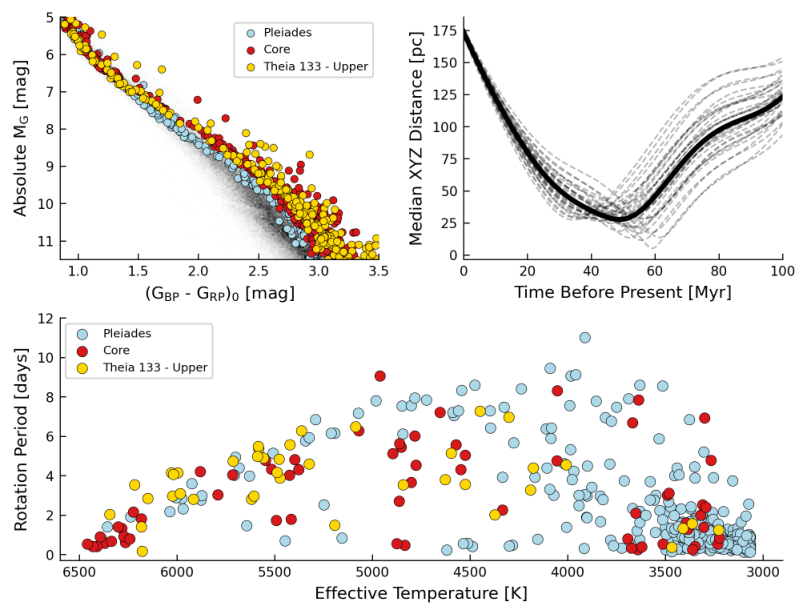

Figure 10 shows that the rotation sequence for stars in this extended upper region overlaps with Per’s sequence, indicating the two regions are approximately coeval. To further analyze whether these two regions are related, we used galpy (Bovy 2015) and MWPotential2014 to back-integrate both the median positions of each region for 100 Myr. galpy is a galactic dynamics software package that allows the user to model the evolution of orbiting bodies in various gravitational potentials. The potential we used is MWPotential2014, which is a simple and accurate model of the Milky Way’s potential and is a combination of individual potentials for each of the Milky Way’s bulge, disk, and dark matter halo. The results are shown in the upper-right panel of Figure 10: Per’s core and the upper extension came within 30 pc of each other 45–50 Myr ago. In other words, these two groups were at least a factor of five closer together in the past, which strongly suggests that they are related to each other. See Appendix B and Figure 18 for additional discussion on the viability of our back-integrations at young ages. We additionally investigated using LAMOST metallicity measurements to constrain the metallicity of this region but found that LAMOST coverage in this region is sparse and so exclude LAMOST measurements from this part of the analysis.
As an additional check on the upper region, we plotted Per, the Pleiades, and the upper region on a CAMD in the upper-left panel of Figure 10. Per is younger than the Pleiades so has more stars on the pre-main-sequence, meaning that it lies above the Pleiades on the CAMD. The upper region lies directly on top of Per’s CAMD sequence, indicating that, like the rotation sequence, the two regions are roughly co-eval.
The median UVW velocity of the upper region differs from that of Per’s core by 4.8 km s-1. To determine whether coeval groups of stars could have a velocity difference of this magnitude by the age of Per, we performed the following numerical experiment. First, to determine a representative starting position and velocity for the core of Per, we manually selected members of the core using the Glueviz software package (Beaumont et al. 2015; Robitaille et al. 2017), calculated their median position and velocity, and then back-integrated for 100 Myr using galpy’s built-in MWPotential2014 potential. Glueviz is a software package that allows the user to manually interact with and visualize differences between large data sets. We then defined 1000 test particles in the vicinity of this starting location, and gave them UVW velocities drawn from a uniform distribution ranging between -1 and 1 km s-1 around the starting UVW velocity of Per’s core. We also required the total UVW velocity to always fall in a 0.01 km s-1 range around 1 km s-1. Each particle was then integrated forward in time to present day. The velocity difference between Per’s median UVW velocity and the UVW velocity of each test particle was calculated at each step of the integration. We then calculated the median UVW velocity difference between the test particles and Per at each step to show how the velocity distribution evolved over time. This procedure was repeated for initial UVW velocity differences of 1.5, 2, 2.5, and 3 km s-1. Figure 11 shows the results. Objects that were born at the location of Per with an initial velocity difference of 1 km s-1 from Per will have a velocity difference of almost 2 km s-1 after 100 Myr. Similarly, stars with an initial velocity difference of 3 km s-1 will have a velocity difference of nearly 6 km s-1 today.
The implication of Figure 11 is that the present-day UVW velocity difference between the core of Per and the upper-region of Theia 133 is physically plausible given an initial velocity difference of 2 km . The observed dispersions of young stellar associations easily allows such a difference (Gagné & Faherty 2018). The combination of overlapping rotation and color–absolute magnitude sequences, the small relative velocity difference, and the two regions coming within 30 pc of each other in the past, strongly suggests that the upper region and Per are indeed related. Once field contaminants have been removed, there are 333 stars in this region (with a total mass of ), with the lowest-mass star having an absolute = 15.25 mags (Pecaut & Mamajek 2013, ;).

Theia 133: Lower
Kounkel & Covey 2019 reported an additional region that lags behind Per in XY space, which was also partially recovered by Kerr et al. 2021. To investigate whether this lower region is related to Per, we performed a similar analysis as for the upper extension to Per. To define this region’s spatial extent, we used Glueviz to manually divide it from the rest of the cluster and removed stars that also overlap with POB3-2, Meingast et al.’s tidal tails, the upper extension, and Per’s core. As can be seen in Figure 6, we recovered periods for 209 of the 341 stars that were expected to have rotation periods in this region. These rotation periods are plotted against the rotation sequence of both Per’s core and the Pleiades in Figure 12. The lower region’s slow sequence lies below that of the Pleiades and overlaps with that of Per. Plus, the transition from increasing rotation periods to decreasing rotation periods occurs at hotter temperatures in this region than in the Pleiades, indicating Per and this lower region have similar ages. As an additional check on age, we plot the stars that have rotation periods on a CAMD. The lower region’s sequence on the CAMD overlaps with Per’s and also indicates they have similar ages.
Groups of stars originating from the same molecular cloud should have the same chemical composition. To explore whether or not this lower region and Per are co-chemical, we employed LAMOST DR7 metallicities (Cui et al. 2012). After searching LAMOST DR7 LRS data for matches with stars in our sample, we found that LAMOST has measurements for 55 stars in this region. When the lower region’s metallicity measurements are plotted over metallicity measurements for Per’s core (Figure 12), we find that the sequences overlap, indicating that the two regions share similar metallicities.
As we did for the upper extension, we performed a back-integration for the lower extension. We again used only stars that are rotationally-consistent with Per membership and back-integrate the median position and velocity of the core and the lower extension. The median XYZ distance between the core and the lower extension over the last 100 Myr is shown in the upper-right panel in Figure 12 and shows that the two regions have remained spatially close over the last 100 Myr, with their distance from each other never increasing or decreasing by more than pc.
Finally, the lower region’s median UVW velocity is separated from the median UVW velocity of Per’s core by only 1.1 km s-1. Taken together, the lower region’s rotation periods, CAMD, metallicity, back-integration, and velocity provide strongly suggestive evidence that the lower region is related to Per. This region contains 660 stars for a total mass of .
VIII.2 Per’s Tidal Tails

We then turned our attention to the diffuse groups reported by Meingast et al. 2021 to lead and lag the core of the cluster. For brevity, we call these the tidal tails, though their tidal origin has yet to be confirmed. Figure 6 shows that rotationally-consistent cluster members are clearly present in these regions. To more accurately define stars inside and outside of Per’s tidal tails, we adopted the tidal radius of 10.0 pc from Meingast et al. 2021, which they defined as the radius where the cluster volume density drops below the density in the field. We therefore assumed that any cluster members residing within a 10 pc radius around the center of the core were members of the core and any cluster members residing more than 10 pc from the center of the core were “corona” or tidal tail members. We compare Per’s core sequence on a CAMD to that of the tidal tails and the Pleiades in the upper-left panel in Figure 13. The CAMD sequence of the core and the tidal tails overlaps and is elevated above the Pleiades’ sequence, indicating that the core and the tidal tails are coeval and younger than the Pleiades.
The rotation sequence of the tidal tails is plotted in the lower-left panel in Figure 13. Like the CAMD, the rotation sequence of Meingast et al. 2021’s tidal tails overlaps with Per’s slow and fast sequences, indicating that the tails and Per’s core are coeval. Their positioning below the Pleiades and turn over at hotter temperatures than the Pleiades indicates that both the core and the tidal tails are younger than the Pleiades.
We also compare LAMOST DR7 metallicity measurements for Per’s core and tidal tails in the lower-right panel in Figure 13. The metallicity sequence of the tails and the core overlap, indicating that the stars in each region share similar metallicities. As a final step, we back-integrated the median position and velocity of both the leading and trailing tidal tails. We defined the leading tail as consisting of all stars that are more than 10 pc away from the center of the core in the direction of galactic rotation and the trailing tail as all stars that are more than 10 pc away from the center of the core in the opposite direction of galactic rotation. We find that the median position of each tail was further away from Per’s core in the past — a finding that is at odds with the idea that the tails formed via evaporation. The upper-right and center-right panels in Figure 13 show the median distance between the core and each tail over the last 100 Myr.
These rotation periods, combined with the kinematic and spatial clustering analysis performed by Meingast et al., the overlapping sequences on the CAMD, and similar LAMOST metallicity sequences, suggest that the tidal tails are related to Per. The back-integration shows the tidal tails moving further away from Per’s core in the past. Possible explanations for this behavior will be discussed in Section IX.4.2.
The binary fraction at different locations in the cluster is a final quantity of dynamical interest. Deacon & Kraus 2020 found that the binary fraction in the cores of denser clusters is lower than in the field. If the same holds true here, we would expect Per’s core to have a lower binary fraction than the tails. We estimated the binary fraction in Per using two different tracers. First, we counted how many stars have a Gaia RUWE 1.2. Stassun & Torres 2021 found that Gaia EDR3 RUWE values even slightly in excess of 1.0 may signify unresolved binaries in Gaia. As such, we made a first comparison of how many stars in each region have RUWE values greater than 1.2. Using our sample of rotationally-consistent cluster members, we find that of stars in the core have RUWE compared to in the tails. Binaries can also appear as over-luminous stars on a CAMD, so as a second step we cut out all stars in vs , , and space that lie above Per’s sequence on a CAMD. Combined with the RUWE 1.2 filter, this gives a binary fraction of for the core and for the tails. We therefore conclude that Per’s core does indeed show evidence of having a lower binary fraction than its tidal tails. Accounting for the relevant Poissonian uncertainties and selection effects would be an interesting area for future study.
VIII.3 POB3-2 from Kerr et al. 2021
We broke our analysis of POB3-2 into three parts: refining the velocity difference between Per and POB3-2, analyzing only stars that Kerr et al. 2021 defines as being part of POB3-2, and then additionally considering stars that their clustering analysis identifies as being unclustered members of the POB3 region but that still spatially overlap with POB3-2.
We obtained RV measurements for stars in POB3-2 by querying Gaia DR3 for each of the 74 stars that Kerr defines as comprising POB3-2 and found that 24 of said stars have RV measurements. The RV measurements were then combined with Gaia DR3 right ascension, declination, proper motion, and parallax to derive UVW space velocities for each star. We compared the median UVW space velocity of POB3-2 to that of Per’s core and find that the median velocities of the two regions differ by km s-1 for a total velocity difference of 6.5 km s-1. Referring back to Figure 11, this velocity difference would imply a primordial velocity difference of 3.3 km s-1, assuming that the two structures were initially at the same location. Given the velocity dispersions of young stellar associations, this is high, but not entirely unreasonable (Gagné & Faherty 2018).

We additionally investigated the rotation sequence, back-integration, and metallicities of POB3-2. Of the 74 stars that Kerr identifies as comprising POB3-2, we recovered rotation periods for only 13 stars, only one of which falls on Per’s slow or fast sequence. In Section IV, we recovered rotation periods for 855 out of 5226 total candidates, or of candidates. The recovery rate for POB3-2 is as well. POB3-2’s rotation sequence is plotted in the lower-left panel in Figure 14. Of the 13 stars in POB3-2 with measured rotation periods, only one star passes the possible binary filters defined in Section VI.1 so we plot all 13 stars in the lower-left panel in Figure 14. The back-integration shows that the median position of the stars in POB3-2 for which we were able to obtain a rotation period only increases in the past relative to Per’s median position. The LAMOST metallicity coverage of POB3-2 was sparse and is included for completeness, though we draw no conclusions from it due to the low number of stars with metallicity measurements in this region. The back-integration and metallicity measurements are shown in the upper-right and lower-right panels in Figure 14, respectively.
The CAMD sequence for POB3-2 overlaps with Per’s CAMD sequence, indicating that the two regions share a similar age. However, the back-integration, velocity difference, and lack of stars that overlap with Per’s rotation sequence all cast doubt on POB3-2 being related to Per. If we include the unclustered members of POB3 from Kerr’s analysis, the number of stars for which we were able to derive rotation periods rises to 30 and results in three stars appearing to overlap with Per’s slow sequence. We conclude that POB3-2 (), at least as defined in Kerr et al. 2021, is likely an unrelated population due to its large velocity difference and lack of stars on the slow sequence, but note that there are additional stars present in the area that Kerr et al. 2021 does not consider to be members of POB3-2 but that are rotationally-consistent with Per membership.
IX Discussion
IX.1 White Dwarfs in Per
White dwarfs can be used to provide an independent age estimate for stellar clusters (Hansen et al. 2002, e.g.,). Casewell et al. 2015 used UKIRT and SuperCOSMOS data to identify 14 white dwarf candidates in Per but were unable to confirm any of the candidates as bona fide cluster members. Lodieu et al. 2019 found that two candidates from Casewell et al. 2015 were in their list of kinematic Per candidates, but both candidates lie outside of Per’s tidal radius and have total ages older than the cluster’s age. Miller et al. 2022 searched for candidate white dwarfs that might have escaped from Per in the past and recover two previously-reported candidates (both candidates were also identified by Lodieu et al. 2019 and Heyl et al. 2021) and discover three new white dwarf candidates at distances greater than 100 pc from the center of the cluster. They confirm that three of their five candidates have cooling ages that are consistent with cluster membership and note that all three are more massive than any other cluster member found using Gaia astrometry.
The list of Per candidates defined in Section III can be used to search for additional white dwarf candidates. As such, we cross-match our list of 5226 candidate Per members with the Gentile Fusillo et al. 2021 catalog of white dwarfs in Gaia EDR3 and identify 23 candidate white dwarfs. All 23 of these candidates have probabilities of being a white dwarf in excess of 99 according to Gentile Fusillo et al. 2021. Two of these white dwarfs are also present in the LAMOST DR8 catalog of white dwarfs: Gaia DR3 173927625524478464 and Gaia DR3 435725089313589376. Gentile Fusillo et al. 2021 calculates stellar surface gravity and effective temperature for each star by assuming a pure-H, pure-He, or mixed H/He atmospheric model, and reports parameters for each model. We use wdwarfdate (Kiman et al. 2022), combined with effective temperature and surface gravity measurements from the Gentile Fusillo et al. catalog or LAMOST DR8 (when applicable) to estimate ages for each white dwarf in our sample. We find that four objects have cooling ages younger than our gyrochronology age for Per: Gaia DR3 173927625524478464 (cooling age: Myr; total age: Myr), Gaia DR3 435725089313589376 (cooling age: Myr; total age: Myr), Gaia DR3 244003693457188608 (cooling age: Myr; total age: Myr), and Gaia DR3 439597809786357248 (cooling age: Myr; total age: Myr). The total age for each white dwarf exceeds Per’s age. This brings up three possibilities: these white dwarfs are not true Per members, the white dwarfs are cluster members and the model for their cooling sequence evolution does not account for intrinsic scatter in the population, or our empirical isochrone and gyrochronology ages for Per are incorrect. Given that the isochrone, gyrochronology, and LDB ages for Per all agree, we prefer the explanation that these white dwarfs are not true Per members. Additionally, Gaia DR3 439597809786357248’s total age is only 2- discrepant from Per’s LDB age and empirical isochrone age. Spectroscopic follow-up of Gaia DR3 439597809786357248 would therefore be useful to prove or disprove its association with Per.
IX.2 Per’s Metallicity
As mentioned in Section II, values for Per’s metallicity reported in the literature have ranged from sub-solar (Boesgaard & Friel 1990, -0.054 0.046;) to super-solar (Pöhnl & Paunzen 2010, 0.18;). To further explore its metallicity, we cross-match our list of stars that are rotationally-consistent with Per membership with the LAMOST DR7 LRS Stellar Parameter Catalog of A, F, G and K Stars and LAMOST LRS Catalog of gM, dM, and sdM stars (Luo et al. 2022). The LAMOST metallicity scale is known to systematically vary with effective temperature (Andrews et al. 2022, e.g.,), so we choose to analyze Per’s metallicity by comparing its LAMOST effective temperature vs metallicity sequence to that of the Pleiades and Praesepe. The Hyades were also considered but did not have as complete of coverage in LAMOST as the Pleiades and Praesepe. Figure 15 shows that Praesepe’s sequence falls above that of both Per and the Pleiades, indicating that Praesepe is the most metal-rich cluster of the three. The sequences of both Per and the Pleiades overlap, indicating that they have similar metallicities, though Per’s sequence might lie slightly above that of the Pleiades.
In the same spirit as the differential gyro age in Section VI, we now derive a differential estimate of Per’s metallicity by fitting a polynomial to each cluster’s LAMOST metallicity sequence. If we compare Per’s measured LAMOST metallicities to those estimated by the fit to Praesepe’s sequence, we find that Per’s sequence lies 0.16 dex below Praesepe’s sequence. Assuming a metallicity for Praesepe of dex (D’Orazi et al. 2020), we find that Per has a metallicity of dex (median and 1-sigma). For comparison, if we repeat the same procedure to measure the metallicity of the Pleiades, we find a metallicity of dex (median and 1-sigma), which is nearly identical to the metallicity reported in Soderblom et al. 2009. It therefore appears that Per’s metallicity is marginally super-solar.
IX.3 What is the best method for identifying diffuse stellar structures?
In Section VII, we derived a true-positive rate of Per members from eight independent studies (Appendix A). There are additional metrics besides the true-positive rate that can be used to assess how well a clustering algorithm performs. For example, a receiver operating characteristic curve can be used to show how the true and false positive rates change at different thresholds and so includes more information than just the true positive rate. Similarly, the false-negative rate is important. Moranta et al. 2022 for instance had a very high true-positive rate, but missed the larger complex that other studies recovered. Here, we focus on only the true-positive rate and its implications for the effectiveness of each study.
As noted, Moranta et al. 2022’s study has the highest true-positive rate of the three studies that used an unsupervised clustering algorithm to perform a blind search on Gaia data, likely due to its inclusion of Gaia RV measurements and its full 6D clustering analysis. Kounkel & Covey 2019, Heyl et al. 2021, and Meingast et al. 2021 all identify stellar structures beyond Per’s core, with Meingast et al. having the highest true-positive rate of the three. It follows that these three studies would have naturally have lower true-positive rates than other studies that focus on identifying cluster cores because more field contaminants will be present further away from cluster cores.
Choice of input parameters, clustering algorithm settings, and scaling of physical parameters should all be taken into account when performing a clustering analysis and can affect the outcome of the clustering analysis. The first important consideration is what physical parameters should be used for the analysis. For example, should the clustering analysis be performed with sky-projected, galactocentric, or cylindrical positions and velocities, or some combination? In order for galactocentric and cyclindrical velocities to be calculated, each star needs to have a valid RV measurement, many of which are available in Gaia. One drawback of requiring stars to have a Gaia RV measurement is that this requirement will exclude low-mass stars. That being said, not requiring stars to have RV measurements requires a careful treatment of projection effects. Kerr et al. 2021 performed their clustering analysis in {} space with HDBSCAN and find an additional region potentially related to Per, POB3-2 (see Section VIII.3). However, this region’s lack of rotation periods that overlap with Per’s rotation sequence and large UVW velocity difference from Per’s core indicate that it is likely not related. Meingast et al. 2021 included an excellent discussion of projection effects as part of their analysis.
Additionally, these clustering algorithms often require careful thought when setting the parameters used in the analysis, such as the number of stars allowed per cluster and the radius within which to search for stars. Given that changing these input parameters will change the number, size, and distribution of clusters that the algorithm finds, clustering algorithms are somewhat tautological and need verification through other means (as done in this work). The scaling of physical parameters must also be taken into account. The variance in every dimension needs to be similar in relative units because this is all the clustering algorithm sees. Improper feature scaling will result in the parameters that have a broad range of values governing the clustering results. This can be solved by normalizing the input data so that each input parameter contributes proportionally to the clustering algorithm. Moranta et al. 2022 and Kerr et al. 2021 both discuss how to address scaling velocities and positions so they can be clustered together.
Hunt & Reffert 2021 performed a similar analysis on Gaia DR2 data by searching for clusters in Gaia DR2 data with DBSCAN, HDBSCAN, and Gaussian Mixture Models. They find that of the methods they studied, HDBSCAN is the most effective at recovering true-positive cluster members. This is in agreement with our results since HDBSCAN was used in Moranta et al. 2022 and results in the lowest false-positive rate of all studies included here. However, given that our studies with the lowest and highest true-positive rates both used HDBSCAN, it appears that the choice of physical parameters, clustering settings, and space scaling (as reported above) are just as important of considerations as which clustering algorithm to use.
Lodieu et al. 2019, Heyl et al. 2021, and Jaehnig et al. 2021 all do not use clustering algorithms such as DBSCAN, HDBSCAN, or UPMASK to identify stellar clusters. Lodieu et al.’s and Jaehnig et al.’s samples have true-positive rates that are consistent with Moranta et al. 2022 within uncertainties. However, each of these three studies bases their search off of previously-reported positions and/or membership lists for Per, which likely helps them find true-positive members. Cantat-Gaudin et al. 2018 falls into that same category even though it uses a clustering algorithm.
This provides evidence that although clustering algorithms like DBSCAN, HDBSCAN, and UPMASK can be effective tools for recovering stellar clusters, the methods employed by Lodieu et al. and Jaehnig et al. prove to be equally-effective methods for determining cluster membership that do not rely on unsupervised clustering algorithms. There are also studies not considered here that explore promising clustering techniques, such as combining 3D parameter space with Gaussian Mixture Models and the Mahalanobis distance (Deb et al. 2022), using DBSCAN combined with a neural network trained on Gaia photometry (Castro-Ginard et al. 2022), and using a combination of k-nearest neighbors and Gaussian Mixture Models (Agarwal et al. 2021).
IX.4 What is the true morphology of Per?
In Section VIII, we examined four different proposed extensions to Per and used isochrone ages, gyrochronology ages, LAMOST metallicities, and back-integration to show that nearby regions of similarly-aged stars are related to Per. We now turn our attention to discussing what these findings mean for how each region could have formed.
IX.4.1 Theia 133

In Section VIII.1, we showed that the large, diffuse structures that comprise Theia 133 from Kounkel & Covey 2019 do appear to be related to Per. We now ask: what are these diffuse structures and how did they form?
Our preferred explanation is that Per is part of a dispersed complex of similarly aged stars and that the upper and lower regions are distinct structures within that complex. Clusters can inherit hierarchical structure from their molecular clouds (Grudić et al. 2021, e.g.,). The clouds can have complex shapes, sometimes resembling filaments more than spheres (Großschedl et al. 2018, e.g.,). Our back-integration from Section VIII.1 shows that the core of Per and the median position of the upper region were within 30 pc of each other in the past. This is well within the typical size scales of molecular filaments (Zucker et al. 2018). If the upper region is composed of stars that evaporated from Per’s core, we would expect the upper region to be made primarily of low mass stars due to mass segregation. However, four of the ten highest mass stars in our sample of stars that are rotationally consistent with Per membership are located in the upper region. The observed number of high-mass stars in the upper region could be explained if the upper region formed adjacent to Per, as it would then be its own grouping of stars and not comprised of evaporated stars from Per’s core.
Another possible scenario for forming the upper and lower regions is that the extensions could be part of Per’s tidal tails. The lower extension shares metallicities and both isochronal and gyrochronal ages with Per, so they are likely related. However, the lower region’s back-integration shows that its distance from Per’s core has oscillated by 20 pc over the last 100 Myr while remaining relatively constant. If the lower region is part of Per’s tidal tails, its separation from Per should decrease in the past, which is not what we see. The separation between the upper region and the core does decrease in the past, but does not come within 30 pc of Per’s core, also indicating that it is likely a separate population. Referring to Figure 16, the core, lower extension, and upper extension all appear to be co-moving — another indication that they are related.
We have shown here that Per is part of a complex of similarly aged stars but there are other studies that mention even further extensions. Gagné et al. 2020 found that the Tau association is very likely related to Per, Theia 160, Cas-Tau (David et al. 2018, Cas-Tau was described in), and e Tau and u Tau (Liu et al. 2020, e and u Tau were originally discovered in). Moranta et al. 2022 notes that they find an additional group, Crius 226, which may be related to Per, Theia 133, and Theia 209, and forms a bridge in XY space between Theia 133 and Theia 209. With more and more clustering studies being released, it’s almost certain that additional clusters will be found that appear to be related to Per. It would be very worthwhile to repeat the rotation-based analysis presented here on all clusters that appear to be related to Per in order to gain a better understanding for the true size and morphology of the Persei complex.
IX.4.2 Per’s Tidal Tails
Tidal tails can form due to either gas expulsion or dynamical evaporation (Baumgardt & Kroupa 2007; Dinnbier & Kroupa 2020a). Once star formation in giant molecular clouds forms massive stars, feedback removes most gas and mass from the system, transforming the embedded cluster into an open cluster. During gas expulsion, stars continue to move at their pre-gas expulsion speeds, but since most of the mass has been removed from the system, their outward motions increase. Depending on the star-formation efficiency, clusters can lose as many as 2/3 of their stars during gas expulsion (Dinnbier & Kroupa 2020a, e.g.,). The remaining stars then revirialize before evaporation of low-mass stars becomes the main source of mass-loss in the cluster. Gas expulsion and evaporation then both contribute to the formation of tidal tails.
However, if the tails formed purely from evaporation, they would be comprised of mostly low-mass stars. Due to mass segregation, low-mass stars should preferentially be located in the outer regions of the cluster. -body simulations predict that tidal tails that form only via gas expulsion should not be mass-segregated, while those that form only via dynamical evaporation should be mass-segregated (Dinnbier & Kroupa 2020b). Gas expulsion acts early in a cluster’s life and on all stars regardless of mass, while dynamical evaporation acts only on low mass stars and makes them travel at low speeds so they stay closer to the core.
To explore if the mass distribution of the tails, we interpolate stellar masses from our dereddened and corrected Gaia values using the tables from Pecaut & Mamajek 2013. Figure 17 shows the 50 of tidal tail stars that reside closest to Per’s core in XYZ space are comprised of a higher number of low-mass stars and lower number of high-mass stars, while the opposite is true for the 50 of stars furthest from Per’s core. If the tails formed purely from evaporation, we would expect the least massive stars to be located in the outer reaches of the cluster. Furthermore, our back-integration shows that both the leading and the trailing tails were not closer to the core of the cluster in the past. If the tails formed purely form dynamical evaporation, we would expect the tails to be closer to the cluster in the past. One possible explanation is that the tails themselves are primordial. They are the same age and metallicity as Per’s core so are likely related, but the mass distribution in the tails and their distance from the core in the past mean that the tails could be comprised at least partially of stars that formed in the same vicinity as Per’s core, but not directly a part of it.
The orientation of the tidal tails recovered by Meingast et al. 2021 and here also matches expectations from simulations. The Coriolis force causes tidal tails to be elongated in the direction of galactic rotation (Dinnbier & Kroupa 2020b). As a cluster moves around the Galaxy, stars that are located closer to the galactic center will experience differential rotation and speed up, forming a leading arm tilted towards the galactic center. Both of these features and shown in Figure 13.
IX.5 How do stars rotate at the age of Per?
On the pre-main-sequence (PMS), stars contract until their core pressures and temperatures are sufficient to fuse hydrogen, which marks the beginning of the zero-age main sequence (ZAMS). High-mass stars reach the ZAMS more quickly than low-mass stars. As a star contracts, its rotation rate generally increases due to conservation of angular momentum. An exception that can stall this spin-up is disk-locking, which locks the rotation period of the star to that of the inner disk wall (Koenigl 1991; Rebull et al. 2018). Once on the ZAMS, angular momentum is carried away by magnetized stellar winds, resulting in spin-down (Weber & Davis 1967). For our purposes, there are two factors that affect magnetic braking in the unsaturated regime: the star’s mass and rotation. Magnetic braking has a mass dependence that causes low-mass stars with a radiative and convective envelope to spin-down more quickly than high-mass stars (Barnes & Kim 2010; Johnstone et al. 2015; Ahuir et al. 2020; Matt et al. 2015). This is why the slow sequence has the shape it does — once on the main-sequence, high mass stars take much longer to spin down than low-mass stars, leading to the trend of increasing rotation period with decreasing mass at a given age.
Internal angular momentum transport may also affect stellar rotation rates (Spada & Lanzafame 2020). As PMS stars contract, radiative cores begin to develop and partially replace the already-existing convective cores (Kunitomo et al. 2017; Spada & Lanzafame 2020). In the early-PMS, the radiative and convective zones rotate together, making the star roughly a rigid body. However, at the end of the PMS phase, wind braking is at its most efficient and internal angular momentum transport between the radiative and convective zones cannot keep up with the angular momentum loss from wind-braking, leading to differential rotation between the two zones (Spada & Lanzafame 2020). This differential rotation persists for the early-main sequence before internal rotational coupling again becomes more efficient than wind-braking. It is the interplay of these two modes of angular momentum transport that is currently the preferred explanation for the stalled spin-down seen in older clusters such as Praesepe and NGC 6811 (Curtis et al. 2020; Spada & Lanzafame 2020). Per is at an age where wind-braking is expected to be dominant over rotational-coupling at every mass range considered. As such, the observed spin-down seen at effective temperatures 5000K in Figure 4 is due to wind-braking, with lower mass stars losing angular momentum more quickly due to the mass-dependence of wind-braking.
Per’s observed rotation periods increase as temperature decreases until temperatures of 5000K. At this temperature, stars have already converged onto the main-sequence where PMS contraction has stopped and wind-braking is the dominant effect, thereby leading to angular momentum loss and decreasing rotation periods. At temperatures between 4500K and 5000K, the scatter in Per’s observed rotation periods increases and erases the slow sequence seen at hotter temperatures. This temperature range corresponds to a color range of . Figure 3 shows that this color range corresponds to the color at which Per stars are just beginning to arrive on the ZAMS, meaning that wind-braking and PMS contraction are both affecting stellar rotation. This transition appears to happen at 4500K for the Pleiades, 4000K for Group X and NGC 3532, and 3500K for Praesepe and follows the arrival of each cluster’s low-mass stars on the ZAMS. At temperatures below 4500K, rotation periods once again decrease because stars have not yet reached the main-sequence so PMS contraction dominates over magnetic braking, leading to short rotation periods. The apparent scatter in rotation periods at 4500K indicates that these stars still contain the rotation information imprinted on them at birth and have yet to lose significant angular momentum.
As stars age, magnetic braking carries away more and more angular momentum, resulting in slower rotation periods at a given mass in older stars. This trend is confirmed here. Per, the youngest cluster in Figure 4 at 79 Myr, has a slow sequence that lies below that of the other clusters in the figure. Because Per is younger than the other clusters, magnetic braking has not had a chance to slow stellar rotation as much as it has for the other clusters, leaving Per’s stars to rotate faster at a given mass than in other clusters. The trend mentioned in Godoy-Rivera et al. 2021 that, at a given mass in the saturated regime, the difference in rotation rates between fast and slow rotators increases with age is also recovered in Figure 4. The difference between the fastest and slowest rotators in Praesepe between 3000K and 3500K is in excess of 20 days, compared to 7.5 days for similar rotators at the age of the Pleiades. This suggests that, at a fixed mass, rapid rotators lose less angular momentum than slow rotators in the saturated regime. Per’s M-dwarfs also appear to have longer rotation periods than stars in the 120 Myr age range. This is because the M-dwarfs at Per’s age have not had as much time to contract as stars in the Pleiades, leading to longer rotation periods.
As noted in several other studies (Meibom et al. 2007; Bouma et al. 2021; Kounkel et al. 2022, e.g.,), the fast sequence is mostly comprised of binaries. There are four stars from the Pleiades, three from Per, and one from Group X that are fast rotators but that survived our binarity filter. One potential explanation for this is disk-locking. In stellar systems with disks, the magnetic field lines from the star can thread the disk, exerting a torque that prevents the star from undergoing PMS contraction. Once the disk dissipates, the star is then free to contract. It is possible that the six stars on the fast sequence in Figure 4 had disks with longer than average lifetimes and so underwent PMS contraction at a later time than other stars in the cluster, resulting in a faster rotation period at a given mass than would otherwise be expected.
X Conclusion
TESS rotation periods have been combined with Gaia photometry and astrometry to analyze the Persei open cluster. Our main conclusions are as follows:
- 1.
By Per’s age, single stars hotter than 5000K (K2V, 0.8) have formed a slow sequence. If we assume an LDB age for Per of Myr (Galindo-Guil et al. 2022), we derive a braking index of 0.51 for stars of this age and effective temperature. At temperatures below 4500K, stars of Per’s age are still on the pre-main-sequence, and at temperatures between 4500K and 5000K, the competing effects of PMS contraction and magnetic spin-down lead to a large variance in observed rotation periods. A 1 star will take Myr to arrive on the ZAMS, while a 0.6 star will take Myr (Choi et al. 2016). At the age of Per, a star with mass 0.75 (K) will have just arrived on the ZAMS; it appears some additional time is required for such stars to reach the slow-rotator sequence.
- 2.
Per is part of a larger complex of similarly-aged stars. Three regions appear to be related to the core of Per: a lower extension (), upper extension (), and the tidal tails as reported by Meingast et al. 2021 (). The lower extension has the same metallicity, isochrone age, and gyrochrone age as Per, and its separation from Per’s core seems to not have significantly changed over the last 100 Myr. The upper extension similarly shares isochrone and gyrochrone ages with Per. Even though the upper extension is currently 175 pc from the core of the cluster, it was five times closer 45–50 Myr ago. The “tidal tails” have the expected metallicity, isochrone, and gyrochrone ages, but their back-integration is inconsistent with the expected signature of expansion; they may be primordial. The lack of mass segregation between the tidal tails and core is a separate line of evidence that supports this possibility.
- 3.
The most effective clustering analyses leverage Gaia’s full 6D position and velocity data to identify bona fide cluster members. True cluster members can be recovered with a high true-positive rate using multiple different clustering algorithms, so the choices of which parameters to use when clustering, the settings adopted in the clustering itself, and how the input data is scaled matter just as much — if not more — than the specific algorithm used.
- 4.
The metallicity of Per is consistent with the Pleaides within 1-. We use LAMOST DR7 LRS spectra to derive a metallicity for Per of dex.
This analysis makes Per a new benchmark cluster for studies on the evolution of stellar rotation. It also provides a new lower anchor for when gyrochronology begins to become applicable. Beyond stellar rotation, our understanding of Persei itself is far from complete. With multiple studies now arguing that additional groups are related to the core of Per, it is clear that more work is needed to understand the full extent and morphology of the complex. Disentangling how the present-day configuration of Per was produced by a mix of its primordial structure and dynamical processing remains an exciting prospect for future work.
Appendix A Descriptions of Each Study’s Clustering Analysis
A.1 Cantat-Gaudin et al. 2018
Cantat-Gaudin et al. 2018 used Gaia DR2 data to derive membership lists and mean parameters for 1229 clusters. The authors started by compiling a list of known clusters and their candidates from previously published catalogs and papers (Dias et al. 2002; Kharchenko et al. 2013, for Per:). A cone search centered on the cluster position from the literature was then performed and all stars with phot_g_mean_mag 18 and a parallax within 0.5 mas of their expected parallax were kept. The authors noted that Per has a large apparent proper motion dispersion and applied no additional constraints on proper motion before running the cluster through the membership assignment code UPMASK. UPMASK uses k-means clustering to identify small groups of stars in 3D astrometric space (, , ). A “veto” step was then performed where the groups identified by UPMASK were compared to a random distribution and a binary yes/no was returned if the group was more/less concentrated than the random distribution. To determine membership probability, the authors performed the grouping and vetoing step multiple times, each time redrawing new values of , , and . This procedure was run 10 times and produced a final list of 873 candidate Per members.
A.2 Kounkel Covey 2019
Kounkel & Covey 2019 used Gaia DR2 to derive shapes and ages for clusters, associations, and comoving groups within 1 kpc and 30 degrees. Their search focused on the galactic mid-plane and extended solar neighborhood between 100 and 1000 pc. Unlike some other papers in our sample (Cantat-Gaudin et al. 2018; Meingast et al. 2021), Kounkel & Covey 2019 did not perform a literature search to get initial positions and/or velocities for stellar clusters. Instead, they applied a series of filters to the full Gaia DR2 sample ( 30 degrees, parallax 1 mas, and six other quality cuts) to derive a sample of 19.55 million stars. The 5D data set of galactic coordinates and , parallax, and proper motion from this sample was then run through HDBSCAN. They then iterated over several different parallax cuts to improve sensitivity to associations between 100 pc and 1000 pc from the Sun. The authors noted that the galactic coordinate grid is discontinuous at degrees and that some structures that cross this boundary became artificially split. For the structures that became split, the authors performed multiple runs of HDBSCAN for different ranges of and manually stitched their results together. Kounkel & Covey 2019 found 2643 members of Per (which they designated as Theia 133).
A.3 Lodieu et al. 2019
Lodieu et al. 2019 used a combination of Gaia DR2 data and previously published literature data to provide updated distances, kinematics, and membership lists for Per, the Pleiades, and Praesepe. The authors combined membership lists from 13 previously published surveys of Per to make a collection of candidate members, which they crossmatched with Gaia DR2 and kept only those with high-quality astrometry (parallax 1 mas, RUWE 1.4). To determine cluster membership, the authors used the kinematic procedure from Perryman et al. 1998. Briefly, this procedure involved transforming Gaia parallaxes into distances, calculating the barycenter and space velocity of the cluster, then estimating the expected transverse and radial velocities at the position of each candidate member. Candidates were selected if they had velocities within of the common cluster motion. Any outliers were then discarded before the mean cluster barycenter and velocity were recalculated. This process was repeated until no outliers remain. The authors calculated the tidal radius of Per (9.5 pc) and reported as their candidates all stars that passed the kinematic procedure outlined above and that were within three times the tidal radius of Per, for a total of 2069 stars. We note that the authors reported all of their candidates, regardless of distance to the center of Per, in their list of Per candidates available online. There are 3162 stars available in this table. In the this analysis, we only used the 517 candidates that Lodieu marked as being within the tidal radius of Per unless otherwise specified.
A.4 Heyl et al. 2021
Heyl et al. 2021 used Gaia EDR3 to determine past and present cluster members for Per, NGC 2451A, IC 2391, and IC 2602. The authors started by conducting two cone searches centered on Per’s position from Gaia Collaboration et al. 2018. The aim of the two cone searches was to construct a complete sphere of radius 60 pc around the cluster with a narrow cone and a complete hemisphere of radius 90 pc on the nearside of the cluster with a broad cone. In the case of Per, this selected all objects in Gaia EDR3 within 250 pc of the sun that lie within 28 degrees of Per on the sky and a second region within 200 pc of the sun and within 45 degrees of the cluster on the sky. The mean cluster position and velocity were then calculated and the sample of candidate stars was defined to be all stars within 10 pc of the cluster center that have proper motions within 5 mas yr-1 of the cluster’s median proper motion. Projection effects were not accounted for. An additional analysis was then performed to look for stars that have escaped from Per. This was done by calculating the velocity of each star relative to Per and its distance from Per as a function of time. These values were then compared to the star’s current position, with the reasoning being that each star has to have moved to its current position within the lifetime of Per. They found 1336 candidate Per members.
A.5 Jaehnig et al. 2021
Jaehnig et al. 2021 used Extreme Deconvolution Gaussian Mixture Models (XDGMM) and Gaia DR2 data to characterize 420 previously reported clusters and discover 11 new clusters. They began by compiling a list of clusters from Ahumada & Lapasset 2007, Dias et al. 2002, and Kharchenko et al. 2013. The candidates for each cluster came from a Gaia DR2 search with a target field of view centered on the cluster’s median position from these three studies and an opening angle equal to 1.5 times the largest cluster angular diameter from the same studies. Any targets with proper motion more than 10 sigma away from the cluster median were removed and only the 10,000 stars with the highest probability of being cluster members based off of their parallax were kept. Proper motions and parallax were then scaled to create an appropriate shape in parameter space before the XDGMM fit is performed. Each cluster was fit nine times with anywhere between 2 and 10 Gaussian components and the best fit was chosen according to the Bayesian Information Criterion. The differential entropy, a measure of the compactness of each Gaussian component, was then calculated and the component with the lowest differential entropy was designated as the cluster component. Individual membership probabilities were then calculated using bootstrap re-sampling on the selected Gaussian component. This procedure identified 601 Per candidates. We note that the membership list from Jaehnig et al. 2021 does not contain any unique candidates (i.e. all of the stars contained in Jaehnig’s membership list are also contained in the seven other studies included in our sample).
A.6 Kerr et al. 2021
Kerr et al. 2021 used Gaia DR2 and HDBSCAN to create the deepest and most comprehensive study of young stellar associations in the local neighborhood to date. The authors created their sample of Gaia DR2 objects by selecting all objects in Gaia DR2 with a parallax 3 mas and imposing quality cuts on unit weight error, BP/RP flux excess factor, visibility periods, and flux error to define a clean sample of candidates with reliable photometric measurements. In order to confirm that a star is young, a model population of 10 million stars was created that allows factors that could affect the photometric youth of a star, such as metallicity, multiplicity, and reddening, to be taken into account. Posterior distributions in mass and age were generated in the sample population corresponding to the locations of each star in the Gaia DR2 population, and the probability that each star is a young star was then estimated by integrating the age posterior over all ages less than 50 Myr. Stars with a probability of being a young star greater than 0.1 then underwent an additional parallax cut to create a final sample of 28,340 stars. The galactocentric XYZ positions and and tangential velocities for each star were then run through HDBSCAN. A total of 27 young associations were found in this population. HDBSCAN was then re-run on 10 of these populations that show visible substructure in order to characterize the hierarchical structures in each region. This process gave 1853 candidates in the Per region.
A.7 Meingast et al. 2021
Meingast et al. 2021 used Gaia DR2 data to determine the morphology and dynamical structure of 10 nearby ( 500 pc) and young (30–300 Myr) open star clusters with Gaia DR2 data, one of which is Per. To start, the authors computed the mean cluster position and velocity of alpha per by using only stars from Cantat-Gaudin et al. 2018 that were designated as Per members and had membership probabilities greater than 0.8. All stars that fell within a large box (300 pc in X, 500 pc in Y, and 100 pc in Z) centered on the mean cluster position were then designated as candidates. Any candidate with a velocity greater than 1.5 km/s away from the bulk cluster velocity was filtered out and DBSCAN was used to extract overdensities in XYZ space from the remaining sample. The authors note that measurement errors in geometric distances along the line of sight resulted in elongated cluster structures. This issue was addressed by using extreme deconvolution to obtain deconcolved distances and, therefore, a more accurate shape for Per. Meingast et al. 2021 reported 1223 stars in Per and estimated there to be 91 field star contaminants in their sample.
A.8 Moranta et al. 2022
Moranta et al. 2022 used HDBSCAN with full 6-dimensional XYZ galactic positions and UVW space velocities of stars within 200 pc from Gaia EDR3 to identify 50 previously known associations, 32 new stellar streams, 9 extensions of groups recovered by Kounkel & Covey 2019, and 8 new coronae. The authors defined their sample by selecting only stars in Gaia EDR3 with parallax above 5 mas and RUWE 3. The XYZ and UVW positions, velocities, and their respective uncertainties were then calculated with a Monte Carlo simulation and stars with uncertainties greater than 3 pc or 3 km s-1 were rejected, creating a sample of 303,540 stars. The UVW velocities of each star in the sample were given the same dimensions as the XYZ positions through a transformation (multiplying each UVW velocity by 12 pc/km s-1) before the stars were run through HDBSCAN, where the authors placed more importance on the kinematic distribution of the cluster than the spatial distribution. This procedure found 165 Per candidates.
Appendix B Back-integrations at Young Ages
As can be seen in Figure 10, Per’s core and the upper extension reached their minimum separation of 30 pc around 50 Myr ago. Beyond 50 Myr ago, the separation between the two regions increases. Why? When embedded clusters are born, the vast majority of mass in the cluster is contained in the gas itself, with only a few percent of the cloud’s mass eventually being converted into stars. As the cluster ages, the gas that is not used in the star formation process is expelled. The model that we used for our back integrations only takes into account the Milky Way’s potential and does not take into account the gravitational potential of the gas from the early stages of the cluster’s life. The extra mass from the gas contributes to the cluster’s gravitational potential and should overwhelm the gravitational potential of the Milky Way at close enough distances from the core, rendering the back integration inaccurate at the young ages when the core and upper extension were closest together.
To quantify this effect, we compared the potential of a point source with molecular cloud-like masses to the potential of the Milky Way at Per’s distance from the center of the Milky Way ( pc). Both potentials were modeled in galpy with MWPotential2014 for the Milky Way’s potential and KeplerPotential for the point source’s potential. KeplerPotential is the galpy implementation of a standard point source potential. For each mass in a range of masses from to , we calculated the point source’s potential and iterated outwards in distance until the point source’s potential was smaller than the Milky Way’s potential. The results of this procedure are displayed in Figure 18 and show that for the core and upper extension’s minimum separation of 30 pc, a cloud would be needed to overcome the Milky Way’s potential. This is roughly double the mass of the Taurus GMC (Larson 1981) and, given that Taurus is known to have on the order of hundreds of members (Kounkel & Covey 2019; Kerr et al. 2021, see e.g.) instead of thousands of members like Per, this appears to be a very reasonable mass requirement.
Appendix C Selection Function

We provide four different ways to select members of our Per sample in Table 3:
- 1.
flag_quality_period: selects the 938 stars that pass our automated and manual quality checks on rotation period.
- 2.
manual_check = g: selects the 863 stars that pass our manual vetting.
- 3.
flag_benchmark_period: selects the 593 stars that pass our binary checks defined in Section VI.1.
- 4.
in_gyro_sample: selects the 238 stars that are used to calibrate gyrochronology.
Figure 19 shows the effect of each of these selection functions in rotation-effective temperature space.
Appendix D Supplementary Figures

We additionally include diagnostic plots for all 855 stars with a rotation period measurement that passed our automated quality checks and 131 additional stars that are included in our set of stars used to calibrate gyrochronology. An example is given in Figure 20. Basic information about each star is plotted in the upper-left panel. The CDIPS light curve is plotted in the upper-right panel with a horizontal red bar to indicate the rotation period. The GLS and PDM periodograms and light curves phase folded on the period from the three most prominent peaks in each periodogram are shown in the next rows. Dashed vertical red lines in the periodogram mark the location of double and half of the period measured by each method. The lower-left panel is the star’s location on Per’s rotation–color diagram and the bottom-right panel is the star’s location on a CAMD, with the grey points representing field stars and black points representing all 986 stars with a rotation period measurement that passed our automated quality checks or that was included in our gyrochronology sample.
References
- Agarwal et al. (2021) Agarwal, M., Rao, K. K., Vaidya, K., & Bhattacharya, S. 2021, MNRAS, 502, 2582, doi: 10.1093/mnras/stab118
- Agüeros et al. (2018) Agüeros, M. A., Bowsher, E. C., Bochanski, J. J., et al. 2018, ApJ, 862, 33, doi: 10.3847/1538-4357/aac6ed
- Ahuir et al. (2020) Ahuir, J., Brun, A. S., & Strugarek, A. 2020, A&A, 635, A170, doi: 10.1051/0004-6361/201936974
- Ahumada & Lapasset (2007) Ahumada, J. A., & Lapasset, E. 2007, A&A, 463, 789, doi: 10.1051/0004-6361:20054590
- André et al. (2014) André, P., Di Francesco, J., Ward-Thompson, D., et al. 2014, in Protostars and Planets VI, ed. H. Beuther, R. S. Klessen, C. P. Dullemond, & T. Henning, 27, doi: 10.2458/azu_uapress_9780816531240-ch002
- Andrews et al. (2022) Andrews, J. J., Curtis, J. L., Chanamé, J., et al. 2022, AJ, 163, 275, doi: 10.3847/1538-3881/ac6952
- Angus et al. (2018) Angus, R., Morton, T., Aigrain, S., Foreman-Mackey, D., & Rajpaul, V. 2018, MNRAS, 474, 2094, doi: 10.1093/mnras/stx2109
- Astropy Collaboration et al. (2013) Astropy Collaboration, Robitaille, T. P., Tollerud, E. J., et al. 2013, A&A, 558, A33, doi: 10.1051/0004-6361/201322068
- Astropy Collaboration et al. (2018) Astropy Collaboration, Price-Whelan, A. M., Sipőcz, B. M., et al. 2018, AJ, 156, 123, doi: 10.3847/1538-3881/aabc4f
- Astropy Collaboration et al. (2022) Astropy Collaboration, Price-Whelan, A. M., Lim, P. L., et al. 2022, apj, 935, 167, doi: 10.3847/1538-4357/ac7c74
- Barnes (2003) Barnes, S. A. 2003, ApJ, 586, 464, doi: 10.1086/367639
- Barnes (2007) —. 2007, ApJ, 669, 1167, doi: 10.1086/519295
- Barnes & Kim (2010) Barnes, S. A., & Kim, Y.-C. 2010, ApJ, 721, 675, doi: 10.1088/0004-637X/721/1/675
- Baumgardt & Kroupa (2007) Baumgardt, H., & Kroupa, P. 2007, MNRAS, 380, 1589, doi: 10.1111/j.1365-2966.2007.12209.x
- Beaumont et al. (2015) Beaumont, C., Goodman, A., & Greenfield, P. 2015, in Astronomical Society of the Pacific Conference Series, Vol. 495, Astronomical Data Analysis Software an Systems XXIV (ADASS XXIV), ed. A. R. Taylor & E. Rosolowsky, 101
- Bhattacharya et al. (2022) Bhattacharya, S., Rao, K. K., Agarwal, M., Balan, S., & Vaidya, K. 2022, MNRAS, doi: 10.1093/mnras/stac2906
- Bhatti et al. (2019) Bhatti, W., Bouma, L., & Yee, S. 2019, waqasbhatti/cdips-pipeline: cdips-pipeline v0.1.0, 0.1.0, Zenodo, Zenodo, doi: 10.5281/zenodo.3370324
- Bhatti et al. (2017) Bhatti, W., Bouma, L. G., & Wallace, J. 2017, Astrobase, Zenodo, doi: 10.5281/zenodo.1185231
- Binney & Tremaine (2008) Binney, J., & Tremaine, S. 2008, Galactic Dynamics: Second Edition
- Boesgaard & Friel (1990) Boesgaard, A. M., & Friel, E. D. 1990, ApJ, 351, 467, doi: 10.1086/168484
- Boffin et al. (2022) Boffin, H. M. J., Jerabkova, T., Beccari, G., & Wang, L. 2022, MNRAS, 514, 3579, doi: 10.1093/mnras/stac1567
- Bossini et al. (2015) Bossini, D., Miglio, A., Salaris, M., et al. 2015, MNRAS, 453, 2290, doi: 10.1093/mnras/stv1738
- Bouma et al. (2021) Bouma, L. G., Curtis, J. L., Hartman, J. D., Winn, J. N., & Bakos, G. Á. 2021, AJ, 162, 197, doi: 10.3847/1538-3881/ac18cd
- Bouma et al. (2019) Bouma, L. G., Hartman, J. D., Bhatti, W., Winn, J. N., & Bakos, G. Á. 2019, ApJS, 245, 13, doi: 10.3847/1538-4365/ab4a7e
- Bouma et al. (2022) Bouma, L. G., Curtis, J. L., Masuda, K., et al. 2022, AJ, 163, 121, doi: 10.3847/1538-3881/ac4966
- Bovy (2015) Bovy, J. 2015, ApJS, 216, 29, doi: 10.1088/0067-0049/216/2/29
- Boyajian et al. (2012) Boyajian, T. S., von Braun, K., van Belle, G., et al. 2012, ApJ, 757, 112, doi: 10.1088/0004-637X/757/2/112
- Brewer et al. (2016) Brewer, J. M., Fischer, D. A., Valenti, J. A., & Piskunov, N. 2016, ApJS, 225, 32, doi: 10.3847/0067-0049/225/2/32
- Burke et al. (2020) Burke, C. J., Levine, A., Fausnaugh, M., et al. 2020, TESS-Point: High precision TESS pointing tool, Astrophysics Source Code Library, record ascl:2003.001. http://ascl.net/2003.001
- Cantat-Gaudin et al. (2018) Cantat-Gaudin, T., Jordi, C., Vallenari, A., et al. 2018, A&A, 618, A93, doi: 10.1051/0004-6361/201833476
- Capitanio et al. (2017) Capitanio, L., Lallement, R., Vergely, J. L., Elyajouri, M., & Monreal-Ibero, A. 2017, A&A, 606, A65, doi: 10.1051/0004-6361/201730831
- Carpenter et al. (2000) Carpenter, J. M., Heyer, M. H., & Snell, R. L. 2000, ApJS, 130, 381, doi: 10.1086/317352
- Casewell et al. (2015) Casewell, S. L., Dobbie, P. D., Geier, S., Lodieu, N., & Hambly, N. C. 2015, MNRAS, 451, 4259, doi: 10.1093/mnras/stv1280
- Castro-Ginard et al. (2022) Castro-Ginard, A., Jordi, C., Luri, X., et al. 2022, A&A, 661, A118, doi: 10.1051/0004-6361/202142568
- Chaussidon (2007) Chaussidon, M. 2007, in Lectures in Astrobiology, ed. M. Gargaud, H. Martin, & P. Claeys, 45, doi: 10.1007/978-3-540-33693-8_2
- Chen et al. (2003) Chen, L., Hou, J. L., & Wang, J. J. 2003, AJ, 125, 1397, doi: 10.1086/367911
- Choi et al. (2016) Choi, J., Dotter, A., Conroy, C., et al. 2016, ApJ, 823, 102, doi: 10.3847/0004-637X/823/2/102
- Cole-Kodikara et al. (2022) Cole-Kodikara, E. M., Barnes, S. A., Weingrill, J., & Granzer, T. 2022, arXiv e-prints, arXiv:2207.11063. https://arxiv.org/abs/2207.11063
- Cui et al. (2012) Cui, X.-Q., Zhao, Y.-H., Chu, Y.-Q., et al. 2012, Research in Astronomy and Astrophysics, 12, 1197, doi: 10.1088/1674-4527/12/9/003
- Curtis et al. (2019a) Curtis, J. L., Agüeros, M. A., Douglas, S. T., & Meibom, S. 2019a, ApJ, 879, 49, doi: 10.3847/1538-4357/ab2393
- Curtis et al. (2019b) Curtis, J. L., Agüeros, M. A., Mamajek, E. E., Wright, J. T., & Cummings, J. D. 2019b, AJ, 158, 77, doi: 10.3847/1538-3881/ab2899
- Curtis et al. (2020) Curtis, J. L., Agüeros, M. A., Matt, S. P., et al. 2020, ApJ, 904, 140, doi: 10.3847/1538-4357/abbf58
- Dahm (2015) Dahm, S. E. 2015, ApJ, 813, 108, doi: 10.1088/0004-637X/813/2/108
- Dalessandro et al. (2021) Dalessandro, E., Varri, A. L., Tiongco, M., et al. 2021, ApJ, 909, 90, doi: 10.3847/1538-4357/abda43
- David & Hillenbrand (2015) David, T. J., & Hillenbrand, L. A. 2015, ApJ, 804, 146, doi: 10.1088/0004-637X/804/2/146
- David et al. (2018) David, T. J., Mamajek, E. E., Vanderburg, A., et al. 2018, AJ, 156, 302, doi: 10.3847/1538-3881/aaeed7
- Deacon & Kraus (2020) Deacon, N. R., & Kraus, A. L. 2020, MNRAS, 496, 5176, doi: 10.1093/mnras/staa1877
- Deb et al. (2022) Deb, S., Baruah, A., & Kumar, S. 2022, MNRAS, 515, 4685, doi: 10.1093/mnras/stac2116
- Dias et al. (2002) Dias, W. S., Alessi, B. S., Moitinho, A., & Lépine, J. R. D. 2002, A&A, 389, 871, doi: 10.1051/0004-6361:20020668
- Dinnbier & Kroupa (2020a) Dinnbier, F., & Kroupa, P. 2020a, A&A, 640, A84, doi: 10.1051/0004-6361/201936570
- Dinnbier & Kroupa (2020b) —. 2020b, A&A, 640, A85, doi: 10.1051/0004-6361/201936572
- Dobbie et al. (2010) Dobbie, P. D., Lodieu, N., & Sharp, R. G. 2010, MNRAS, 409, 1002, doi: 10.1111/j.1365-2966.2010.17355.x
- Donahue et al. (1996) Donahue, R. A., Saar, S. H., & Baliunas, S. L. 1996, ApJ, 466, 384, doi: 10.1086/177517
- D’Orazi et al. (2020) D’Orazi, V., Oliva, E., Bragaglia, A., et al. 2020, A&A, 633, A38, doi: 10.1051/0004-6361/201936651
- Douglas et al. (2017) Douglas, S. T., Agüeros, M. A., Covey, K. R., & Kraus, A. 2017, ApJ, 842, 83, doi: 10.3847/1538-4357/aa6e52
- Douglas et al. (2019) Douglas, S. T., Curtis, J. L., Agüeros, M. A., et al. 2019, ApJ, 879, 100, doi: 10.3847/1538-4357/ab2468
- Eddington (1910) Eddington, A. S. 1910, MNRAS, 71, 43, doi: 10.1093/mnras/71.1.43
- Ester et al. (1996) Ester, M., Kriegel, H.-P., Sander, J., & Xu, X. 1996, in Proceedings of the Second International Conference on Knowledge Discovery and Data Mining, KDD’96 (AAAI Press), 226–231
- Fodera-Serio et al. (1985) Fodera-Serio, G., Indorato, L., & Nastasi, P. 1985, Journal for the History of Astronomy, 16, 1
- Foreman-Mackey et al. (2017) Foreman-Mackey, D., Agol, E., Ambikasaran, S., & Angus, R. 2017, AJ, 154, 220, doi: 10.3847/1538-3881/aa9332
- Foreman-Mackey et al. (2021) Foreman-Mackey, D., Luger, R., Agol, E., et al. 2021, exoplanet: Gradient-based probabilistic inference for exoplanet data & other astronomical time series, 0.5.1, Zenodo, doi: 10.5281/zenodo.7191939
- Fritzewski et al. (2020) Fritzewski, D. J., Barnes, S. A., James, D. J., & Strassmeier, K. G. 2020, A&A, 641, A51, doi: 10.1051/0004-6361/201936860
- Fritzewski et al. (2021) —. 2021, A&A, 652, A60, doi: 10.1051/0004-6361/202140894
- Gagné et al. (2020) Gagné, J., David, T. J., Mamajek, E. E., et al. 2020, ApJ, 903, 96, doi: 10.3847/1538-4357/abb77e
- Gagné & Faherty (2018) Gagné, J., & Faherty, J. K. 2018, ApJ, 862, 138, doi: 10.3847/1538-4357/aaca2e
- Gagné et al. (2021) Gagné, J., Faherty, J. K., Moranta, L., & Popinchalk, M. 2021, ApJ, 915, L29, doi: 10.3847/2041-8213/ac0e9a
- Gaia Collaboration et al. (2016) Gaia Collaboration, Prusti, T., de Bruijne, J. H. J., et al. 2016, A&A, 595, A1, doi: 10.1051/0004-6361/201629272
- Gaia Collaboration et al. (2018) Gaia Collaboration, Babusiaux, C., van Leeuwen, F., et al. 2018, A&A, 616, A10, doi: 10.1051/0004-6361/201832843
- Gaia Collaboration et al. (2021) Gaia Collaboration, Smart, R. L., Sarro, L. M., et al. 2021, A&A, 649, A6, doi: 10.1051/0004-6361/202039498
- Gaia Collaboration et al. (2022) Gaia Collaboration, Vallenari, A., Brown, A. G. A., et al. 2022, arXiv e-prints, arXiv:2208.00211. https://arxiv.org/abs/2208.00211
- Galindo-Guil et al. (2022) Galindo-Guil, F. J., Barrado, D., Bouy, H., et al. 2022, A&A, 664, A70, doi: 10.1051/0004-6361/202141114
- Gallet & Bouvier (2015) Gallet, F., & Bouvier, J. 2015, A&A, 577, A98, doi: 10.1051/0004-6361/201525660
- Gentile Fusillo et al. (2021) Gentile Fusillo, N. P., Tremblay, P. E., Cukanovaite, E., et al. 2021, MNRAS, 508, 3877, doi: 10.1093/mnras/stab2672
- Gillen et al. (2020) Gillen, E., Briegal, J. T., Hodgkin, S. T., et al. 2020, MNRAS, 492, 1008, doi: 10.1093/mnras/stz3251
- Godoy-Rivera et al. (2021) Godoy-Rivera, D., Pinsonneault, M. H., & Rebull, L. M. 2021, ApJS, 257, 46, doi: 10.3847/1538-4365/ac2058
- Gordon et al. (2021) Gordon, T. A., Davenport, J. R. A., Angus, R., et al. 2021, ApJ, 913, 70, doi: 10.3847/1538-4357/abf63e
- Großschedl et al. (2018) Großschedl, J. E., Alves, J., Meingast, S., et al. 2018, A&A, 619, A106, doi: 10.1051/0004-6361/201833901
- Grudić et al. (2021) Grudić, M. Y., Kruijssen, J. M. D., Faucher-Giguère, C.-A., et al. 2021, MNRAS, 506, 3239, doi: 10.1093/mnras/stab1894
- Gruner & Barnes (2020) Gruner, D., & Barnes, S. A. 2020, A&A, 644, A16, doi: 10.1051/0004-6361/202038984
- Hansen et al. (2002) Hansen, B. M. S., Brewer, J., Fahlman, G. G., et al. 2002, ApJ, 574, L155, doi: 10.1086/342528
- Healy & McCullough (2020) Healy, B. F., & McCullough, P. R. 2020, ApJ, 903, 99, doi: 10.3847/1538-4357/abbc03
- Heyl et al. (2021) Heyl, J., Caiazzo, I., Richer, H., & Miller, D. R. 2021, arXiv e-prints, arXiv:2110.04296. https://arxiv.org/abs/2110.04296
- Hodierna (1654) Hodierna, G. B. 1654, De systemate orbis cometici deque admirandis coeli characteribus explicantur, necnon vie Com etarum, per orbem cometicum multiplices opuscula duo, in quorum primo cometarum causae disquiruntur, & indicantur. In secundo vero quid, quales, quotue sint stellae luminosae, nebulae, necnon, & occultae, manifestantur & rerum caelestium studiosis commendantur, doi: 10.3931/e-rara-444
- Holcomb et al. (2022) Holcomb, R. J., Robertson, P., Hartigan, P., Oelkers, R. J., & Robinson, C. 2022, ApJ, 936, 138, doi: 10.3847/1538-4357/ac8990
- Horne & Baliunas (1986) Horne, J. H., & Baliunas, S. L. 1986, ApJ, 302, 757, doi: 10.1086/164037
- Hunt & Reffert (2021) Hunt, E. L., & Reffert, S. 2021, A&A, 646, A104, doi: 10.1051/0004-6361/202039341
- Hunter (2007) Hunter, J. D. 2007, Computing in Science & Engineering, 9, 90, doi: 10.1109/MCSE.2007.55
- Jaehnig et al. (2021) Jaehnig, K., Bird, J., & Holley-Bockelmann, K. 2021, ApJ, 923, 129, doi: 10.3847/1538-4357/ac1d51
- Jerabkova et al. (2021) Jerabkova, T., Boffin, H. M. J., Beccari, G., et al. 2021, A&A, 647, A137, doi: 10.1051/0004-6361/202039949
- Johnstone et al. (2015) Johnstone, C. P., Güdel, M., Brott, I., & Lüftinger, T. 2015, A&A, 577, A28, doi: 10.1051/0004-6361/201425301
- Kerr et al. (2021) Kerr, R. M. P., Rizzuto, A. C., Kraus, A. L., & Offner, S. S. R. 2021, ApJ, 917, 23, doi: 10.3847/1538-4357/ac0251
- Kharchenko et al. (2013) Kharchenko, N. V., Piskunov, A. E., Schilbach, E., Röser, S., & Scholz, R. D. 2013, A&A, 558, A53, doi: 10.1051/0004-6361/201322302
- Kiman et al. (2022) Kiman, R., Xu, S., Faherty, J. K., et al. 2022, AJ, 164, 62, doi: 10.3847/1538-3881/ac7788
- Koenigl (1991) Koenigl, A. 1991, ApJ, 370, L39, doi: 10.1086/185972
- Kounkel & Covey (2019) Kounkel, M., & Covey, K. 2019, AJ, 158, 122, doi: 10.3847/1538-3881/ab339a
- Kounkel et al. (2022) Kounkel, M., Stassun, K. G., Bouma, L. G., et al. 2022, AJ, 164, 137, doi: 10.3847/1538-3881/ac866d
- Kounkel et al. (2018) Kounkel, M., Covey, K., Suárez, G., et al. 2018, AJ, 156, 84, doi: 10.3847/1538-3881/aad1f1
- Kraus et al. (2017) Kraus, A. L., Herczeg, G. J., Rizzuto, A. C., et al. 2017, ApJ, 838, 150, doi: 10.3847/1538-4357/aa62a0
- Krolikowski et al. (2021) Krolikowski, D. M., Kraus, A. L., & Rizzuto, A. C. 2021, AJ, 162, 110, doi: 10.3847/1538-3881/ac0632
- Krone-Martins & Moitinho (2014) Krone-Martins, A., & Moitinho, A. 2014, A&A, 561, A57, doi: 10.1051/0004-6361/201321143
- Krumholz et al. (2019) Krumholz, M. R., McKee, C. F., & Bland-Hawthorn, J. 2019, ARA&A, 57, 227, doi: 10.1146/annurev-astro-091918-104430
- Kunitomo et al. (2017) Kunitomo, M., Guillot, T., Takeuchi, T., & Ida, S. 2017, A&A, 599, A49, doi: 10.1051/0004-6361/201628260
- Lada & Lada (2003) Lada, C. J., & Lada, E. A. 2003, ARA&A, 41, 57, doi: 10.1146/annurev.astro.41.011802.094844
- Lallement et al. (2018) Lallement, R., Capitanio, L., Ruiz-Dern, L., et al. 2018, A&A, 616, A132, doi: 10.1051/0004-6361/201832832
- Lamers et al. (2010) Lamers, H. J. G. L. M., Baumgardt, H., & Gieles, M. 2010, MNRAS, 409, 305, doi: 10.1111/j.1365-2966.2010.17309.x
- Lamm et al. (2004) Lamm, M. H., Bailer-Jones, C. A. L., Mundt, R., Herbst, W., & Scholz, A. 2004, A&A, 417, 557, doi: 10.1051/0004-6361:20035588
- Larson (1981) Larson, R. B. 1981, MNRAS, 194, 809, doi: 10.1093/mnras/194.4.809
- Liu et al. (2020) Liu, J., Fang, M., & Liu, C. 2020, AJ, 159, 105, doi: 10.3847/1538-3881/ab6b22
- Lodieu et al. (2019) Lodieu, N., Pérez-Garrido, A., Smart, R. L., & Silvotti, R. 2019, A&A, 628, A66, doi: 10.1051/0004-6361/201935533
- Lomb (1976) Lomb, N. R. 1976, Ap&SS, 39, 447, doi: 10.1007/BF00648343
- Long et al. (2005) Long, M., Romanova, M. M., & Lovelace, R. V. E. 2005, ApJ, 634, 1214, doi: 10.1086/497000
- Luo et al. (2022) Luo, A. L., Zhao, Y. H., Zhao, G., & et al. 2022, VizieR Online Data Catalog, V/156
- Mamajek & Hillenbrand (2008) Mamajek, E. E., & Hillenbrand, L. A. 2008, ApJ, 687, 1264, doi: 10.1086/591785
- Mann et al. (2015) Mann, A. W., Feiden, G. A., Gaidos, E., Boyajian, T., & von Braun, K. 2015, ApJ, 804, 64, doi: 10.1088/0004-637X/804/1/64
- Matt et al. (2015) Matt, S. P., Brun, A. S., Baraffe, I., Bouvier, J., & Chabrier, G. 2015, ApJ, 799, L23, doi: 10.1088/2041-8205/799/2/L23
- McInnes et al. (2017) McInnes, L., Healy, J., & Astels, S. 2017, The Journal of Open Source Software, 2, doi: 10.21105/joss.00205
- Meibom et al. (2007) Meibom, S., Mathieu, R. D., & Stassun, K. G. 2007, ApJ, 665, L155, doi: 10.1086/521437
- Meingast et al. (2021) Meingast, S., Alves, J., & Rottensteiner, A. 2021, A&A, 645, A84, doi: 10.1051/0004-6361/202038610
- Melotte (1915) Melotte, P. J. 1915, MmRAS, 60, 175
- Mermilliod (1981) Mermilliod, J. C. 1981, A&A, 97, 235
- Messina et al. (2010) Messina, S., Desidera, S., Turatto, M., Lanzafame, A. C., & Guinan, E. F. 2010, A&A, 520, A15, doi: 10.1051/0004-6361/200913644
- Messina et al. (2022) Messina, S., Nardiello, D., Desidera, S., et al. 2022, A&A, 657, L3, doi: 10.1051/0004-6361/202142276
- Miller et al. (2022) Miller, D. R., Caiazzo, I., Heyl, J., Richer, H. B., & Tremblay, P.-E. 2022, ApJ, 926, L24, doi: 10.3847/2041-8213/ac50a5
- Moranta et al. (2022) Moranta, L., Gagné, J., Couture, D., & Faherty, J. K. 2022, arXiv e-prints, arXiv:2206.04567. https://arxiv.org/abs/2206.04567
- Murakami et al. (2022) Murakami, Y. S., Jennings, C., Hoffman, A. M., et al. 2022, MNRAS, 514, 4489, doi: 10.1093/mnras/stac1538
- Netopil et al. (2016) Netopil, M., Paunzen, E., Heiter, U., & Soubiran, C. 2016, A&A, 585, A150, doi: 10.1051/0004-6361/201526370
- O’dell & Collier Cameron (1993) O’dell, M. A., & Collier Cameron, A. 1993, MNRAS, 262, 521, doi: 10.1093/mnras/262.2.521
- Pamos Ortega et al. (2022) Pamos Ortega, D., García Hernández, A., Suárez, J. C., et al. 2022, MNRAS, 513, 374, doi: 10.1093/mnras/stac864
- pandas development team (2022) pandas development team, T. 2022, pandas-dev/pandas: Pandas 1.4.3, v1.4.3, Zenodo, doi: 10.5281/zenodo.6702671
- Pecaut & Mamajek (2013) Pecaut, M. J., & Mamajek, E. E. 2013, ApJS, 208, 9, doi: 10.1088/0067-0049/208/1/9
- Perryman et al. (1998) Perryman, M. A. C., Brown, A. G. A., Lebreton, Y., et al. 1998, A&A, 331, 81. https://arxiv.org/abs/astro-ph/9707253
- Pöhnl & Paunzen (2010) Pöhnl, H., & Paunzen, E. 2010, A&A, 514, A81, doi: 10.1051/0004-6361/200810855
- Popinchalk et al. (2022) Popinchalk, M., Faherty, J. K., Curtis, J. L., et al. 2022, arXiv e-prints, arXiv:2211.05258. https://arxiv.org/abs/2211.05258
- Prosser & Grankin (1997) Prosser, C. F., & Grankin, K. N. 1997, Rotation Periods of Open Cluster Stars. IV., Center for Astrophysics Preprint Series No. 4539, 12 pages
- Prosser et al. (1993) Prosser, C. F., Shetrone, M. D., Marilli, E., et al. 1993, PASP, 105, 1407, doi: 10.1086/133322
- Prosser et al. (1995) Prosser, C. F., Shetrone, M. D., Dasgupta, A., et al. 1995, PASP, 107, 211, doi: 10.1086/133541
- Rampalli et al. (2021) Rampalli, R., Agüeros, M. A., Curtis, J. L., et al. 2021, ApJ, 921, 167, doi: 10.3847/1538-4357/ac0c1e
- Randich et al. (2018) Randich, S., Tognelli, E., Jackson, R., et al. 2018, A&A, 612, A99, doi: 10.1051/0004-6361/201731738
- Rebull et al. (2018) Rebull, L. M., Stauffer, J. R., Cody, A. M., et al. 2018, AJ, 155, 196, doi: 10.3847/1538-3881/aab605
- Rebull et al. (2016) Rebull, L. M., Stauffer, J. R., Bouvier, J., et al. 2016, AJ, 152, 113, doi: 10.3847/0004-6256/152/5/113
- Reinhold & Hekker (2020) Reinhold, T., & Hekker, S. 2020, A&A, 635, A43, doi: 10.1051/0004-6361/201936887
- Ricker et al. (2015) Ricker, G. R., Winn, J. N., Vanderspek, R., et al. 2015, Journal of Astronomical Telescopes, Instruments, and Systems, 1, 014003, doi: 10.1117/1.JATIS.1.1.014003
- Robitaille et al. (2017) Robitaille, T., Beaumont, C., Qian, P., Borkin, M., & Goodman, A. 2017, glueviz v0.13.1: multidimensional data exploration, 0.13.1, Zenodo, doi: 10.5281/zenodo.1237692
- Ryden (2016) Ryden, B. 2016, Dynamics, Ohio State Graduate Astrophysics Series (Office of Distance Ed & eLearning at OSU). https://books.google.com/books?id=DAOYCwAAQBAJ
- Skumanich (1972) Skumanich, A. 1972, ApJ, 171, 565, doi: 10.1086/151310
- Soderblom et al. (2009) Soderblom, D. R., Laskar, T., Valenti, J. A., Stauffer, J. R., & Rebull, L. M. 2009, AJ, 138, 1292, doi: 10.1088/0004-6256/138/5/1292
- Spada & Lanzafame (2020) Spada, F., & Lanzafame, A. C. 2020, A&A, 636, A76, doi: 10.1051/0004-6361/201936384
- Spitzer (1958) Spitzer, Lyman, J. 1958, ApJ, 127, 17, doi: 10.1086/146435
- Stassun & Torres (2021) Stassun, K. G., & Torres, G. 2021, ApJ, 907, L33, doi: 10.3847/2041-8213/abdaad
- Stauffer et al. (2016) Stauffer, J., Rebull, L., Bouvier, J., et al. 2016, AJ, 152, 115, doi: 10.3847/0004-6256/152/5/115
- Stauffer et al. (1989) Stauffer, J. R., Hartmann, L. W., & Jones, B. F. 1989, ApJ, 346, 160, doi: 10.1086/167996
- Stauffer et al. (1987) Stauffer, J. R., Schild, R. A., Baliunas, S. L., & Africano, J. L. 1987, PASP, 99, 471, doi: 10.1086/132007
- Stauffer et al. (1999) Stauffer, J. R., Barrado y Navascués, D., Bouvier, J., et al. 1999, ApJ, 527, 219, doi: 10.1086/308069
- Stellingwerf (1978) Stellingwerf, R. F. 1978, ApJ, 224, 953, doi: 10.1086/156444
- VanderPlas (2018) VanderPlas, J. T. 2018, ApJS, 236, 16, doi: 10.3847/1538-4365/aab766
- Virtanen et al. (2020) Virtanen, P., Gommers, R., Oliphant, T. E., et al. 2020, Nature Methods, 17, 261, doi: 10.1038/s41592-019-0686-2
- Weber & Davis (1967) Weber, E. J., & Davis, Leverett, J. 1967, ApJ, 148, 217, doi: 10.1086/149138
- Wes McKinney (2010) Wes McKinney. 2010, in Proceedings of the 9th Python in Science Conference, ed. Stéfan van der Walt & Jarrod Millman, 56 – 61, doi: 10.25080/Majora-92bf1922-00a
- Wright & Mamajek (2018) Wright, N. J., & Mamajek, E. E. 2018, MNRAS, 476, 381, doi: 10.1093/mnras/sty207
- Zechmeister & Kürster (2009) Zechmeister, M., & Kürster, M. 2009, A&A, 496, 577, doi: 10.1051/0004-6361:200811296
- Zucker et al. (2018) Zucker, C., Battersby, C., & Goodman, A. 2018, ApJ, 864, 153, doi: 10.3847/1538-4357/aacc66