Real-time quantum error correction beyond break-even
Abstract
The ambition of harnessing the quantum for computation is at odds with the fundamental phenomenon of decoherence. The purpose of quantum error correction (QEC) is to counteract the natural tendency of a complex system to decohere. This cooperative process, which requires participation of multiple quantum and classical components, creates a special type of dissipation that removes the entropy caused by the errors faster than the rate at which these errors corrupt the stored quantum information. Previous experimental attempts to engineer such a process faced an excessive generation of errors that overwhelmed the error-correcting capability of the process itself. Whether it is practically possible to utilize QEC for extending quantum coherence thus remains an open question. We answer it by demonstrating a fully stabilized and error-corrected logical qubit whose quantum coherence is significantly longer than that of all the imperfect quantum components involved in the QEC process, beating the best of them with a coherence gain of . We achieve this performance by combining innovations in several domains including the fabrication of superconducting quantum circuits and model-free reinforcement learning.
Implementing a single correctable logical qubit requires a physical system with a large state space. It should accommodate the code subspace and its redundant replicas where the logical information will be displaced without distortion when physical errors occur Knill and Laflamme 1997. This redundancy is inextricably associated with an additional operational cost of QEC, known as the control overhead. In the search for an efficient way to alleviate its detrimental effects, bosonic codes Gottesman et al. 2001; Mirrahimi et al. 2014; Michael et al. 2016; Grimsmo et al. 2020 based on the state space of a harmonic oscillator have been proposed as a promising alternative to the standard approach based on registers of physical qubits Shor 1995; Steane 1996; Fowler et al. 2012. In hybrid architectures, these two approaches are complementary, with qubit-register codes built upon logical qubits dynamically protected with efficient base-layer bosonic QEC Noh and Chamberland 2020; Darmawan et al. 2021; Terhal et al. 2020.
Although some aspects of QEC have been demonstrated with superconducting circuits Ofek et al. 2016; Hu et al. 2019; Campagne-Ibarcq et al. 2020; Gertler et al. 2021; Krinner et al. 2022; Zhao et al. 2022; Sundaresan et al. 2022; Acharya et al. 2022, trapped ions de Neeve et al. 2022; Ryan-Anderson et al. 2021; Egan et al. 2021, and spins in solid-state systems Waldherr et al. 2014; Abobeih et al. 2022; Xue et al. 2022, the control overhead prevents current-day experiments from getting to the heart of what QEC promises to achieve – extending the lifetime of quantum information stored in the system. This extension is quantified by the gain , defined as the ratio between the coherence time of an actively error-corrected logical qubit and the best passive qubit encoding in the same system. The break-even point is reached at . A bosonic cat-code experiment Ofek et al. 2016 managed to achieved , but with a code that continuously shrinks to the vacuum state. Other experiments with various bosonic codes Hu et al. 2019; Campagne-Ibarcq et al. 2020; Gertler et al. 2021 and qubit-register codes Krinner et al. 2022; Zhao et al. 2022; Sundaresan et al. 2022; Acharya et al. 2022 have achieved .
We demonstrate full code stabilization and error correction with gain using the Gottesman-Kitaev-Preskill (GKP) encoding Gottesman et al. 2001 of a logical qubit into grid states of an oscillator. The QEC of this code was previously realized in superconducting circuits Campagne-Ibarcq et al. 2020 and trapped ions de Neeve et al. 2022. In our work, similarly to Campagne-Ibarcq et al. 2020, the oscillator is an electromagnetic mode of a superconducting cavity whose quantum state is manipulated using a transmon ancilla, see Fig. 1(a). Our system has an average relaxation and dephasing time of and for the tantalum-based transmon Place et al. 2021, and and for the high-purity aluminum cavity Reagor et al. 2016. We implement in this system a “trickle-down” QEC scheme based on the proposals in Refs. Royer et al. 2020; de Neeve et al. 2022, which includes real-time classical processing and measurement-based feedback. We train the QEC circuit parameters in-situ with reinforcement learning (RL) Sutton and Barto 2018; Schulman et al. 2017; Guadarrama et al. 2018, ensuring their adaptation to the real error channels and control imperfections of our system. At peak performance, the achieved lifetimes of logical Pauli eigenstates are and , and the logical Pauli error probabilities per QEC cycle are and . With such low logical error probabilities, we explore the QEC process on a previously inaccessible time scale of thousands of cycles, subjecting to scrutiny the standard assumptions of the theory of QEC, such as the stationarity of error rates and absence of leakage-induced correlations. Finally, we perform error-injection experiments to identify the major factors limiting logical performance and chart the path towards the next-generation logical qubit.

Engineering error correction
We now explain the principles of our experiment. Its core idea is to realize an artificial error-correcting dissipation that removes the entropy from the system in an efficient manner by prioritizing the correction of frequent small errors, while not neglecting rare large errors. This idea is illustrated in Fig. 2(a) for a cartoon system in which redundancy is achieved with only 4 orthogonal subspaces in total, where is the code subspace and are the error subspaces. In this example, the dissipation scheme is maximally efficient from the perspective of entropy removal, since it corrects any error in a single step. Such an approach is taken by all qubit-register stabilizer codes, where measurement of the stabilizers, syndrome decoding, and recovery, when composed, realize a dissipation channel of high Kraus rank. Although this approach can also be applied to the oscillator grid code (see Methods), its implementation entails large control overhead, which in practice might bring more errors than it is designed to correct. By contrast, the trickle-down dissipation scheme has the capacity to correct all the same errors, but it is not able to do so in a single step. Importantly, the most probable small errors, corresponding to the error space , are still corrected in a single step. Owing to this simplification, such an approach reduces control overhead in the grid code, and therefore it was adopted in our work. The continuous-time version of approach was also demonstrated for other bosonic codes in Lescanne et al. 2020; Gertler et al. 2021.
The stabilizer generators of an ideal square grid code are and , where is the length of a grid unit cell, and is the displacement operator for an oscillator with creation and annihilation operators and . Logical Pauli operators of the ideal code are defined as and . The ideal codewords obey perfect translation symmetry in phase space and thus contain an infinite amount of energy. The finite-energy code is obtained by applying a normalizing envelope operator to the ideal codewords, where parametrizes the code family that approaches the ideal code in the limit. In phase space, this parameter controls the extent of the codewords and the squeezing of their probability peaks. Our experimental Wigner functions of the codewords with are shown in Fig. 1(c). The operators of the finite-energy code are obtained through the similarity transformation induced by the envelope operator Royer et al. 2020, for example, .
To realize an error-correcting dissipation channel for the finite-energy code, there is at our disposal a single ancilla qubit and a classical controller. In principle, with such resources, it is possible to implement arbitrary quantum channels of Kraus rank by recycling the ancilla times and using feedback operations conditioned on the state of the classical -bit memory of the controller Lloyd and Viola 2001; Shen et al. 2017. Here, we construct a rank-4 error correction channel as a composition of two rank-2 dissipators that drive the system towards the eigenspace of the finite-energy code stabilizers . A general rank-2 dissipation can be implemented as a unitary that entangles the system with the ancilla qubit, followed by ancilla projective measurement with outcome , and a classically-conditioned unitary , see Fig. 2(b).
In our experiment, any unitary is compiled down to a set of primitive operations: qubit rotations around any equatorial axis implemented as Gaussian pulses with spectral corrections Chen et al. 2016; oscillator displacements implemented as Gaussian pulses; relatively slow conditional rotations implemented by waiting a certain amount of time under the dispersive coupling Hamiltonian with ; and virtual oscillator rotations implemented dynamically on the field-programmable gate array (FPGA) in . These primitives are used to construct a fast echoed conditional displacement gate as shown in Fig. 2(b), whose speed is enhanced compared to the native interaction strength by a large factor – magnitude of the intermediate displacement in phase space Campagne-Ibarcq et al. 2020; Eickbusch et al. 2021.
Both rank-2 dissipators are then implemented as follows: the unitary is decomposed as a parametrized circuit consisting of layers of qubit rotations and entangling gates, while the unitary is realized as only a virtual rotation, see Fig. 2(b). The role of is twofold: to implement switching between and by changing the quadrature of the oscillator by , and to compensate for a spurious rotation due to the always-on dispersive coupling . The role of is to approximate the mapping of the finite-energy stabilizer onto the state of the ancilla together with autonomous back-action that pushes the state from the error spaces towards the code space. Several ansätze for decomposition of were proposed in Ref. Royer et al. 2020. We adopt a modified version of the so-called small-big-small (SBS) protocol, named to reflect the relative amplitudes of the three conditional displacement gates that it contains: , see Supp. Info. S4.3 for further details.
A single application of the resulting composite dissipator realizes a QEC cycle; we refer to applications of constituent dissipators as evenodd cycles. In our implementation, the duration of a QEC cycle is , which includes execution of unitary gates, ancilla measurements, and real-time processing and decision making by the controller.

Learning QEC circuit parameters
While the SBS ansatz and gate calibrations lead to a functioning QEC process, the highest level of performance cannot be achieved with a crude model of the system based on a few independently calibrated parameters – any such model will inevitably contain unrealistic assumptions. Some model inaccuracies and unknown control imperfections can be compensated by closed-loop optimization with direct feedback from the experimental setup. Previously, pulse-level optimization was successfully utilized to improve gate fidelities Kelly et al. 2014; Rol et al. 2017; Werninghaus et al. 2021; Baum et al. 2021, but it was never applied to enhance the performance of QEC. Here, for the first time, we apply a real-time reinforcement learning agent to this task, as illustrated in Fig. 1(b). We use the proximal policy optimization (PPO) algorithm Schulman et al. 2017; Guadarrama et al. 2018, which was shown in simulations to outperform other approaches on high-dimensional problems with stochastic objective that arise in quantum control Sivak et al. 2022. We parametrize the QEC circuit with parameters that include the amplitudes of various primitive pulses in the circuit decomposition, parameters of the ancilla reset, etc.
The training episodes begin with dissipative pre-cooling of the oscillator followed by feedback cooling to prepare the system ground state , see Methods. Then, a logical Pauli eigenstate or is initialized with a method from Eickbusch et al. 2021, and a candidate QEC protocol is run for cycles. We chose this duration to enhance the signal-to-noise ratio of the reward, similar to the technique used to sample randomized benchmarking cost functions Kelly et al. 2014; Rol et al. 2017; Werninghaus et al. 2021; Baum et al. 2021. At the end of the episode, the reward for the RL agent is obtained by measuring the logical Pauli operator or (depending on the initial state), which provides a proxy for the logical lifetime. This logical measurement is done with one-bit phase estimation of the ideal-code Pauli operators Terhal and Weigand 2016; Campagne-Ibarcq et al. 2020, and its fidelity is intrinsically limited to Terhal et al. 2020. Although there exist methods of logical readout adapted to the finite code envelope Royer et al. 2020; de Neeve et al. 2022; Hastrup and Andersen 2021, we use the phase estimation method to avoid biasing the RL agent towards a particular finite envelope size and to let it pick the optimal size given the error channels of our system.
By construction, the reward incentivizes the RL agent to find a QEC protocol that leads to the longest logical qubit lifetime. The typical evolution of the average reward during the training is shown in Fig. 2(c). The performance level indicated with a black triangle is achieved with independent calibrations of the system and control parameters, see Supp. Info. S2. The RL agent significantly improves upon this baseline performance in two stages: in the first hundred training epochs, the agent corrects large errors in the initial parameter values, and in the subsequent few hundreds of epochs, it fine-tunes the circuit parameters to achieve the highest performance.
Several trends in the learning trajectories highlight the benefits of the model-free RL approach; we elucidate them in more detail in the Supp. Info. S4.4. Here, we only highlight a single illustrative example. In our implementation of the gate, there exists a nontrivial tradeoff between coherent and incoherent errors: the gate can be implemented faster by displacing the oscillator further in phase space, i.e., populating it with more intermediate photons, but this makes the gate more susceptible to high-order nonlinear effects Eickbusch et al. 2021. Moreover, some choices of this intermediate photon number can result in a Stark shift of the ancilla into resonance with a spurious degree of freedom, e.g., a two-level defect Klimov et al. 2018; Lisenfeld et al. 2019. How these tradeoffs translate into logical qubit performance is difficult to model, but the RL agent can learn the optimal value of the large intermediate displacement without a model. As shown in Fig. 2(d), it chose to reduce the intermediate photon number, improving the performance of QEC at the cost of a much slower gate.
Observing QEC beyond break-even

After the training is finished, we pick the best performing QEC circuit for further characterization. Here, we focus on the ability of QEC to create a good quantum memory, i.e. to convert the effect of passage of time into an identity channel that preserves all qubit states.
A metric quantifying the deviation of any quantum channel from the identity is the average channel fidelity, where the integral is over the uniform measure on the qubit state space, normalized so that . In general, this fidelity decays over time in a nontrivial way, but to leading order it evolves as , where the decay rate is equivalent to an average decoherence rate of all pure states on the qubit Bloch sphere. Conveniently, it suffices to average across the six Pauli eigenstates alone Nielsen 2002, leading to an experimental procedure for extracting that can be applied to any kind of qubit irrespective of its error channel. In Fig. 3, we show the results of such an experiment, conducted for three different qubit encodings in our system: the subspace of the transmon, the subspace of the oscillator, and grid code of the oscillator (with and without QEC).
Both the and qubits are subject to amplitude damping and white-noise dephasing channels, captured by their respective and times, with fidelity decay constant given by . From the perspective of a quantum memory, the best uncorrectable physical qubit in our system is , shown in Fig. 3(b), which achieves . The qubit, shown for completeness in Fig. 3(a), only achieves .

Higher excited states of the oscillator have shorter lifetime due to bosonic enhancement of spontaneous emission. Therefore, as with any QEC code, encoding a qubit using grid states incurs an immediate penalty in the fidelity decay rate. Moreover, this natural decay, shown in Fig. 3(c) with empty circles, takes the grid states outside the logical manifold and eventually towards the vacuum state .
Our error correcting dissipation stabilizes the grid code manifold and, together with naturally occurring dissipation, leads to a logical Pauli channel within this manifold, with the lifetimes of logical Pauli eigenstates of and . Under the Pauli channel, the fidelity decay constant is given by , which in our experiment amounts to .
The principal metric characterizing the quality of QEC from the perspective of quantum memory is the coherence gain of an actively error-corrected logical qubit over the best passive qubit encoding. In our experiment, the highest achieved gain is , confidently beyond break-even.
QEC process characterization
Having characterized the logical qubit as a quantum memory, we next examine the properties of the QEC process. Ancilla measurement outcomes, referred to as syndromes, inform us which stochastic path the QEC process has taken in each cycle. In Fig. 4(a) we show a (statistically unrepresentative) sample of these outcomes that comprise trajectories of different experimental shots. Such a dataset contains an immense amount of information about the QEC process, not available in previous experiments with the grid code QEC Campagne-Ibarcq et al. 2020; de Neeve et al. 2022.
To interpret this dataset, we adopt here a simplified model of trickle-down dissipation such as depicted in Fig. 2(a), which captures the essence of our QEC process. The caveats of this model and the exact Kraus decomposition of our QEC circuit are provided in Supp. Info. S4.2. In this simplified model, the outcome indicates that the state was projected onto the code space, while an outcome indicates that the state was transferred one level down the error hierarchy, partially or completely correcting an error.
From the dataset in Fig. 4(a), we observe that the vast majority of outcomes are (green), which means that errors are rare. The stochastic pattern of outcomes (yellow) reflects randomly occurring errors. Most errors are small and, when corrected, leave single isolated outcomes. An example syndrome string likely generated by a large error in one quadrature is indicated with an arrow: it has a characteristic pattern. We also observe isolated ancilla leakage events (red). Leakage to is reset in the same cycle with high probability. Sometimes, leakage persists for multiple cycles (streak of red), due to the transmon escaping to a state higher than , which is not addressed in our reset scheme.
The average probability of each outcome as a function of time is shown Fig. 4(b), where the process starts from a state. After about cycles of initial state correction, the process settles into a dynamical equilibrium which persists for at least a hundred thousand cycles (the longest measured here) without any notable increase of the error rates over time. Detailed analysis reveals that the QEC process is nearly stationary, with residual deviations from stationarity caused by the transmon leakage to states higher than at a rate per cycle, see Supp. Info. S4.6.
In this dynamical equilibrium, physical errors excite the quantum state out of the code space with probability per QEC cycle, as deduced from the statistics of syndrome outcomes. The competition between physical errors and error-correcting dissipation results in a “thermal” distribution across the subspaces with probability of occupying the code space, see Methods. Having justifies the use of low-rank error-correcting dissipation in our system, which is sufficient to prevent physical errors from accumulating and causing logical errors. At the highest achieved QEC gain, the logical Pauli error probabilities per QEC cycle are and . By comparing the total logical error probability, , to the physical error probability , we conclude that of the errors are successfully corrected by our process.
Since rare large errors require several cycles to be corrected, the QEC process is weakly time-correlated with a correlation length of cycles, see Supp. Info. S4.6. To understand these correlations, in Fig. 4(c) we inject displacement errors along the position quadrature and monitor the syndromes that they produce as a function of time. Such errors leave traces of outcomes in proportion to their distance to the closest logical operation. For example, a displacement of length , equivalent to a logical identity, leaves no syndrome trace; a displacement of length is close to a logical bit-flip of the finite-energy code, and hence it leaves only a small syndrome trace; on the other hand, a midway displacement of length makes a large-distance error which takes the longest time to correct with a low-rank dissipator, generating a lasting trace of outcomes.
This displacement error injection experiment confirms that errors indeed generate the syndromes, but do these syndromes herald the occurrence of errors? To verify this, we perform post-selection of trajectories with different syndrome patterns. In particular, we discard trajectories that have consecutive outcomes in the same-quadrature cycles, with resulting post-selected decay of Pauli eigenstates shown in Fig. 4(d). In the case , post-selection eliminates rare large-distance errors and improves the fidelity lifetime only by a factor , but at the cost of rejection probability of per cycle. On the other hand, in the case , post-selection eliminates relatively frequent small errors that are close to identity, as well as rare large uncorrectable errors that are close to a logical operation. It is because of the latter that the fidelity lifetime in this setting improves by a factor , but with a more severe rejection probability of per cycle. These favorable post-selection results indicate that such a method can be used for probabilistic preparation of high-fidelity logical states, including the magic states required for universal quantum computing Bravyi and Kitaev 2005, which is left for future investigation.
Conclusion and Outlook
In this work, we used real-time error correction to realize a fully stabilized logical qubit whose lifetime is more than doubled compared to the best passive qubit encoding in the system, marking the transition of QEC from proof-of-principle studies to a practical tool for enhancing quantum memories. Our work improves upon previous QEC experiments, which do not protect the logical identity operator Ofek et al. 2016, protect only one of the logical Pauli operators or Grimm et al. 2020; Lescanne et al. 2020; Chen et al. 2021, implement correction in post-processing Krinner et al. 2022; Zhao et al. 2022; Acharya et al. 2022, require post-selection Andersen et al. 2020, and do not reach break-even Hu et al. 2019; Gertler et al. 2021; Campagne-Ibarcq et al. 2020; Krinner et al. 2022; Zhao et al. 2022; Acharya et al. 2022. Instrumental for this achievement, among other factors, was the adoption of a model-free learning framework, improved fabrication technique for the ancilla transmon, and a novel grid-code QEC protocol.
Performing additional experiments, we identified the core challenges that need to be addressed to ensure future progress of grid-code QEC. In particular, by studying long-time system stability, we found that occasional collapses of the logical performance are strongly correlated with appearance of spurious degrees of freedom in the system. Their resonant interaction with the Stark-shifted transmon ancilla degrades the fidelity of our operations, see Supp. Info. S4.10. In the short term, this effect could be mitigated by adopting a tunable ancilla and periodically re-training the QEC circuit to find better spectral locations. In the long term, the behavior of these defects needs to be understood, as they pose even greater danger for scaled-up quantum devices Krinner et al. 2022; Zhao et al. 2022; Acharya et al. 2022.
In addition, we expect that considerable enhancement can be gained by tailoring the QEC process not only to error channels of the oscillator, but also those of the ancilla. Our QEC circuit is fault-tolerant with respect to ancilla phase-flip errors by design Royer et al. 2020. With the transmon ancilla used here, the sensitivity of the logical lifetime to ancilla phase flips is times smaller than to ancilla bit flips, as found with noise injection experiments, see Supp. Info. S4.9. Future development should incorporate robustness against ancilla bit flips, either through path-independent control Ma et al. 2020; Rosenblum et al. 2018 or by adopting a biased-noise ancilla Puri et al. 2019.
Acknowledgments
We acknowledge discussions with R. Cortiñas, J. Claes, and A. Mi. This research was supported by the U.S. Army Research Office (ARO) under grants W911NF-18-1-0212 and W911NF-16-1-0349, and by the U.S. Department of Energy, Office of Science, National Quantum Information Science Research Centers, Co-design Center for Quantum Advantage (C2QA) under contract number DE-SC0012704. The views and conclusions contained in this document are those of the authors and should not be interpreted as representing official policies, either expressed or implied, of the U.S. Government. The U.S. Government is authorized to reproduce and distribute reprints for Government purpose notwithstanding any copyright notation herein. Fabrication facilities use was supported by the Yale Institute for Nanoscience and Quantum Engineering (YINQE) and the Yale SEAS Cleanroom.
Author contributions
V.S., A.M. and A.E. built the experimental setup. R.J.S. contributed to experimental apparatus. I.T., S.G. and L.F. fabricated the ancilla transmon chip. B.R., S.S. and S.M.G. developed the theory. B.R., V.S., A.E. and B.B. developed dissipative oscillator cooling. A.E., V.S. and A.Z.D. developed state initialization technique. V.S. implemented reinforcement learning, performed the experiments, and analyzed data. V.S., A.E., B.R. and M.H.D. regularly discussed the project and provided insight. M.H.D. supervised the project. V.S. and M.H.D. wrote the manuscript with feedback from all authors.
Competing interests
R.J.S., L.F. and M.H.D. are founders, and R.J.S. and L.F. are shareholders of Quantum Circuits, Inc.
Methods
QEC of the ideal grid code
To understand error correcting properties of the ideal code, consider an error channel decomposed in the displacement basis. An ideal grid code with code projector satisfies Knill-Laflamme conditions Knill and Laflamme 1997 for all errors in a correctable set . A displacement error of amplitude creates an error state , where is any state from the code space. Since a displaced grid state is still translationally invariant, it remains an eigenstate of the ideal code stabilizers, and the phase of its eigenvalue encodes a continuous error syndrome: and . Error correction of an ideal grid code can be done in a similar manner to any stabilizer code: first, measure the stabilizers to obtain the error syndrome, which here corresponds to phase estimation of that yields the error amplitude . This step projects the state onto one of the orthogonal error spaces. Then, apply the recovery operation, here a simple displacement , to correct the error. Such procedure realizes an artificial dissipation of an infinite rank which corrects any error from in a single cycle, , analogously to the cartoon high-rank dissipation in Fig. 2(a). In contrast to this approach, our experiment realizes low-rank dissipation that asymptotically satisfies .
Dissipative cooling to vacuum
We utilize the dissipation engineering framework Gross et al. 2018 to design fast cooling of the oscillator to vacuum state in the weak-coupling regime where previous known cooling methods Pfaff et al. 2017 fail; we also expect this novel method to be applicable to cooling of trapped ions de Neeve et al. 2022. Similarly to error-correcting dissipation, we realize this cooling as a composition of two rank-2 channels that shrink the oscillator state in the orthogonal quadratures. The unitary in this case is realized as a three-layer circuit obtained from first-order Trotter decomposition of , where controls the cooling rate. This unitary swaps the excitations of the oscillator into the ancilla, which is reset in every cycle. The duration of one full cooling cycle (including both quadratures) is . With , we achieve cooling at a rate times faster than natural energy damping rate of the oscillator. In our experiment, full cycles of such a dissipative cooling are then followed with a feedback cooling protocol adapted from Ofek et al. 2016 to remove any residual thermal population. See Supp. Info. S2.6 for more details.
Reinforcement learning implementation
The QEC circuit is parametrized with a vector . Instead of optimizing directly, the RL agent learns parameters of the probability distribution from which is stochastically sampled during the training to ensure adequate exploration of parameter space. To this end, we use a factorized multivariate Gaussian distribution with mean and covariance matrix . To capture the pattern of relations between different components of , the mean and covariance are represented as parametrized functions and of common hidden variables . In this work, and are produced at the output of a neural network with two fully connected layers of 50 and 20 rectifier linear unit (ReLU) neurons. Starting with initial vector of parameters found with independent calibrations, during the course of learning the agent gradually deforms the distribution and localizes it on the new vector , the final result of the optimization. Typically, as it proceeds, the agent also reduces the covariance of the distribution to have a finer control over the mean. These features of learning are observed in the example evolution of one component of in Fig. 2(d). During one training epoch, we evaluate 10 QEC circuit candidates with 300 episodes (i.e. experimental shots) per candidate. The collected information is used to update the neural network parameters according to the PPO algorithm, which completes the epoch. One epoch takes approximately seconds, with the majority of time spent on re-compilation of FPGA instruction sequences and its re-initialization. See Supp. Info. S3.2 for more details.
Steady state of the QEC process
We perform Wigner tomography of the logical states after varying duration of the QEC process, reconstruct the density matrix, and from its spectral decomposition extract the expectation value of the code projector , where error bar represents the standard deviation with respect to different process durations of , and cycles. In addition to the code space, only one error space is occupied in the steady state with an appreciable probability of . The logical decoherence within this error space happens at the same rate as within the code space. For more details, see Supp. Info. S4.8.
The expectation value of the code projector in the steady state can be estimated independently, using the statistics of syndrome outcomes. Under the approximations discussed in Supp. Info. S4.5, the probability that a syndrome string of length consists only of outcomes asymptotically approaches for large . Using this method, we extract and . The error bar in this case represents the accuracy of the model for the string probability, which is valid to first order in . The value of quoted in the main text is the average of the two methods. Constructing a detailed error budget of the aggregate error probability based on the system-level simulation of the known error processes is an avenue left for future work.
References
- Knill and Laflamme (1997) E. Knill and R. Laflamme, Theory of quantum error-correcting codes, Phys. Rev. A 55, 900 (1997).
- Gottesman et al. (2001) D. Gottesman, A. Kitaev, and J. Preskill, Encoding a qubit in an oscillator, Physical Review A 64, 012310 (2001).
- Mirrahimi et al. (2014) M. Mirrahimi, Z. Leghtas, V. V. Albert, S. Touzard, R. J. Schoelkopf, L. Jiang, and M. H. Devoret, Dynamically protected cat-qubits: a new paradigm for universal quantum computation, New Journal of Physics 16, 045014 (2014).
- Michael et al. (2016) M. H. Michael, M. Silveri, R. T. Brierley, V. V. Albert, J. Salmilehto, L. Jiang, and S. M. Girvin, New class of quantum error-correcting codes for a bosonic mode, Physical Review X 6, 031006 (2016).
- Grimsmo et al. (2020) A. L. Grimsmo, J. Combes, and B. Q. Baragiola, Quantum computing with rotation-symmetric bosonic codes, Physical Review X 10, 011058 (2020).
- Shor (1995) P. W. Shor, Scheme for reducing decoherence in quantum computer memory, Phys. Rev. A 52, R2493 (1995).
- Steane (1996) A. M. Steane, Error correcting codes in quantum theory, Phys. Rev. Lett. 77, 793 (1996).
- Fowler et al. (2012) A. G. Fowler, M. Mariantoni, J. M. Martinis, and A. N. Cleland, Surface codes: Towards practical large-scale quantum computation, Physical Review A 86, 032324 (2012).
- Noh and Chamberland (2020) K. Noh and C. Chamberland, Fault-tolerant bosonic quantum error correction with the surface–Gottesman-Kitaev-Preskill code, Phys. Rev. A 101, 012316 (2020).
- Darmawan et al. (2021) A. S. Darmawan, B. J. Brown, A. L. Grimsmo, D. K. Tuckett, and S. Puri, Practical quantum error correction with the XZZX code and Kerr-cat qubits, PRX Quantum 2, 030345 (2021).
- Terhal et al. (2020) B. M. Terhal, J. Conrad, and C. Vuillot, Towards scalable bosonic quantum error correction, Quantum Science and Technology 5, 043001 (2020).
- Ofek et al. (2016) N. Ofek, A. Petrenko, R. Heeres, P. Reinhold, Z. Leghtas, B. Vlastakis, Y. Liu, L. Frunzio, S. M. Girvin, L. Jiang, et al., Extending the lifetime of a quantum bit with error correction in superconducting circuits, Nature 536, 441 (2016).
- Hu et al. (2019) L. Hu, Y. Ma, W. Cai, X. Mu, Y. Xu, W. Wang, Y. Wu, H. Wang, Y. P. Song, C.-L. Zou, et al., Quantum error correction and universal gate set operation on a binomial bosonic logical qubit, Nature Physics 15, 503 (2019).
- Campagne-Ibarcq et al. (2020) P. Campagne-Ibarcq, A. Eickbusch, S. Touzard, E. Zalys-Geller, N. E. Frattini, V. V. Sivak, P. Reinhold, S. Puri, S. Shankar, R. J. Schoelkopf, et al., Quantum error correction of a qubit encoded in grid states of an oscillator, Nature 584, 368 (2020).
- Gertler et al. (2021) J. M. Gertler, B. Baker, J. Li, S. Shirol, J. Koch, and C. Wang, Protecting a bosonic qubit with autonomous quantum error correction, Nature 590, 243 (2021).
- Krinner et al. (2022) S. Krinner, N. Lacroix, A. Remm, A. Di Paolo, E. Genois, C. Leroux, C. Hellings, S. Lazar, F. Swiadek, J. Herrmann, et al., Realizing repeated quantum error correction in a distance-three surface code, Nature 605, 669 (2022).
- Zhao et al. (2022) Y. Zhao, Y. Ye, H.-L. Huang, Y. Zhang, D. Wu, H. Guan, Q. Zhu, Z. Wei, T. He, S. Cao, et al., Realization of an error-correcting surface code with superconducting qubits, Physical Review Letters 129, 030501 (2022).
- Sundaresan et al. (2022) N. Sundaresan, T. J. Yoder, Y. Kim, M. Li, E. H. Chen, G. Harper, T. Thorbeck, A. W. Cross, A. D. Córcoles, and M. Takita, Matching and maximum likelihood decoding of a multi-round subsystem quantum error correction experiment, arXiv:2203.07205 (2022).
- Acharya et al. (2022) R. Acharya, I. Aleiner, R. Allen, T. I. Andersen, M. Ansmann, F. Arute, K. Arya, A. Asfaw, J. Atalaya, R. Babbush, et al., Suppressing quantum errors by scaling a surface code logical qubit, arXiv:2207.06431 (2022).
- de Neeve et al. (2022) B. de Neeve, T.-L. Nguyen, T. Behrle, and J. P. Home, Error correction of a logical grid state qubit by dissipative pumping, Nature Physics 18, 296 (2022).
- Ryan-Anderson et al. (2021) C. Ryan-Anderson, J. Bohnet, K. Lee, D. Gresh, A. Hankin, J. Gaebler, D. Francois, A. Chernoguzov, D. Lucchetti, N. Brown, et al., Realization of real-time fault-tolerant quantum error correction, Physical Review X 11, 041058 (2021).
- Egan et al. (2021) L. Egan, D. M. Debroy, C. Noel, A. Risinger, D. Zhu, D. Biswas, M. Newman, M. Li, K. R. Brown, M. Cetina, et al., Fault-tolerant control of an error-corrected qubit, Nature 598, 281 (2021).
- Waldherr et al. (2014) G. Waldherr, Y. Wang, S. Zaiser, M. Jamali, T. Schulte-Herbrüggen, H. Abe, T. Ohshima, J. Isoya, J. Du, P. Neumann, et al., Quantum error correction in a solid-state hybrid spin register, Nature 506, 204 (2014).
- Abobeih et al. (2022) M. Abobeih, Y. Wang, J. Randall, S. Loenen, C. Bradley, M. Markham, D. Twitchen, B. Terhal, and T. Taminiau, Fault-tolerant operation of a logical qubit in a diamond quantum processor, Nature 606, 884 (2022).
- Xue et al. (2022) X. Xue, M. Russ, N. Samkharadze, B. Undseth, A. Sammak, G. Scappucci, and L. M. Vandersypen, Quantum logic with spin qubits crossing the surface code threshold, Nature 601, 343 (2022).
- Place et al. (2021) A. P. Place, L. V. Rodgers, P. Mundada, B. M. Smitham, M. Fitzpatrick, Z. Leng, A. Premkumar, J. Bryon, A. Vrajitoarea, S. Sussman, et al., New material platform for superconducting transmon qubits with coherence times exceeding 0.3 milliseconds, Nature communications 12, 1 (2021).
- Reagor et al. (2016) M. Reagor, W. Pfaff, C. Axline, R. W. Heeres, N. Ofek, K. Sliwa, E. Holland, C. Wang, J. Blumoff, K. Chou, et al., Quantum memory with millisecond coherence in circuit QED, Physical Review B 94, 014506 (2016).
- Royer et al. (2020) B. Royer, S. Singh, and S. M. Girvin, Stabilization of finite-energy Gottesman-Kitaev-Preskill states, Physical Review Letters 125, 260509 (2020).
- Sutton and Barto (2018) R. S. Sutton and A. G. Barto, Reinforcement learning: an introduction (A Bradford Book, 2018).
- Schulman et al. (2017) J. Schulman, F. Wolski, P. Dhariwal, A. Radford, and O. Klimov, Proximal policy optimization algorithms, arXiv:1707.06347 (2017).
- Guadarrama et al. (2018) S. Guadarrama, A. Korattikara, O. Ramirez, P. Castro, E. Holly, S. Fishman, K. Wang, E. Gonina, N. Wu, E. Kokiopoulou, et al., TF-Agents: A library for reinforcement learning in tensorflow, https://github.com/tensorflow/agents (2018).
- Lescanne et al. (2020) R. Lescanne, M. Villiers, T. Peronnin, A. Sarlette, M. Delbecq, B. Huard, T. Kontos, M. Mirrahimi, and Z. Leghtas, Exponential suppression of bit-flips in a qubit encoded in an oscillator, Nature Physics 16, 509 (2020).
- Lloyd and Viola (2001) S. Lloyd and L. Viola, Engineering quantum dynamics, Phys. Rev. A 65, 010101 (2001).
- Shen et al. (2017) C. Shen, K. Noh, V. V. Albert, S. Krastanov, M. H. Devoret, R. J. Schoelkopf, S. M. Girvin, and L. Jiang, Quantum channel construction with circuit quantum electrodynamics, Physical Review B 95, 134501 (2017).
- Chen et al. (2016) Z. Chen, J. Kelly, C. Quintana, R. Barends, B. Campbell, Y. Chen, B. Chiaro, A. Dunsworth, A. G. Fowler, E. Lucero, et al., Measuring and suppressing quantum state leakage in a superconducting qubit, Physical Review Letters 116, 020501 (2016).
- Eickbusch et al. (2021) A. Eickbusch, V. Sivak, A. Z. Ding, S. S. Elder, S. R. Jha, J. Venkatraman, B. Royer, S. M. Girvin, R. J. Schoelkopf, and M. H. Devoret, Fast universal control of an oscillator with weak dispersive coupling to a qubit, arXiv:2111.06414 (2021).
- Kelly et al. (2014) J. Kelly, R. Barends, B. Campbell, Y. Chen, Z. Chen, B. Chiaro, A. Dunsworth, A. G. Fowler, I.-C. Hoi, E. Jeffrey, et al., Optimal quantum control using randomized benchmarking, Physical Review Letters 112, 240504 (2014).
- Rol et al. (2017) M. A. Rol, C. C. Bultink, T. E. O’Brien, S. R. de Jong, L. S. Theis, X. Fu, F. Luthi, R. F. L. Vermeulen, J. C. de Sterke, A. Bruno, et al., Restless tuneup of high-fidelity qubit gates, Physical Review Applied 7, 041001 (2017).
- Werninghaus et al. (2021) M. Werninghaus, D. J. Egger, F. Roy, S. Machnes, F. K. Wilhelm, and S. Filipp, Leakage reduction in fast superconducting qubit gates via optimal control, npj Quantum Information 7, 14 (2021).
- Baum et al. (2021) Y. Baum, M. Amico, S. Howell, M. Hush, M. Liuzzi, P. Mundada, T. Merkh, A. R. Carvalho, and M. J. Biercuk, Experimental deep reinforcement learning for error-robust gate-set design on a superconducting quantum computer, PRX Quantum 2, 040324 (2021).
- Sivak et al. (2022) V. V. Sivak, A. Eickbusch, H. Liu, B. Royer, I. Tsioutsios, and M. H. Devoret, Model-free quantum control with reinforcement learning, Physical Review X 12, 011059 (2022).
- Terhal and Weigand (2016) B. M. Terhal and D. Weigand, Encoding a qubit into a cavity mode in circuit QED using phase estimation, Physical Review A 93, 012315 (2016).
- Hastrup and Andersen (2021) J. Hastrup and U. L. Andersen, Improved readout of qubit-coupled Gottesman-Kitaev-Preskill states, Quantum Science and Technology 6, 035016 (2021).
- Klimov et al. (2018) P. V. Klimov, J. Kelly, Z. Chen, M. Neeley, A. Megrant, B. Burkett, R. Barends, K. Arya, B. Chiaro, Y. Chen, et al., Fluctuations of energy-relaxation times in superconducting qubits, Physical Review Letters 121, 90502 (2018).
- Lisenfeld et al. (2019) J. Lisenfeld, A. Bilmes, A. Megrant, R. Barends, J. Kelly, P. Klimov, G. Weiss, J. M. Martinis, and A. V. Ustinov, Electric field spectroscopy of material defects in transmon qubits, npj Quantum Information 5, 1 (2019).
- Nielsen (2002) M. A. Nielsen, A simple formula for the average gate fidelity of a quantum dynamical operation, Physics Letters A 303, 249 (2002).
- Bravyi and Kitaev (2005) S. Bravyi and A. Kitaev, Universal quantum computation with ideal Clifford gates and noisy ancillas, Physical Review A 71, 022316 (2005).
- Grimm et al. (2020) A. Grimm, N. E. Frattini, S. Puri, S. O. Mundhada, S. Touzard, M. Mirrahimi, S. M. Girvin, S. Shankar, and M. H. Devoret, Stabilization and operation of a Kerr-cat qubit, Nature 584, 205 (2020).
- Chen et al. (2021) Z. Chen, K. J. Satzinger, J. Atalaya, A. N. Korotkov, A. Dunsworth, D. Sank, C. Quintana, M. McEwen, R. Barends, P. V. Klimov, et al., Exponential suppression of bit or phase errors with cyclic error correction, Nature 595, 383 (2021).
- Andersen et al. (2020) C. K. Andersen, A. Remm, S. Lazar, S. Krinner, N. Lacroix, G. J. Norris, M. Gabureac, C. Eichler, and A. Wallraff, Repeated quantum error detection in a surface code, Nature Physics 16, 875 (2020).
- Ma et al. (2020) W.-L. Ma, M. Zhang, Y. Wong, K. Noh, S. Rosenblum, P. Reinhold, R. J. Schoelkopf, and L. Jiang, Path-independent quantum gates with noisy ancilla, Physical Review Letters 125, 110503 (2020).
- Rosenblum et al. (2018) S. Rosenblum, P. Reinhold, M. Mirrahimi, L. Jiang, L. Frunzio, and R. J. Schoelkopf, Fault-tolerant detection of a quantum error, Science 361, 266 (2018).
- Puri et al. (2019) S. Puri, A. Grimm, P. Campagne-Ibarcq, A. Eickbusch, K. Noh, G. Roberts, L. Jiang, M. Mirrahimi, M. H. Devoret, and S. M. Girvin, Stabilized cat in a driven nonlinear cavity: A fault-tolerant error syndrome detector, Phys. Rev. X 9, 041009 (2019).
- Gross et al. (2018) J. A. Gross, C. M. Caves, G. J. Milburn, and J. Combes, Qubit models of weak continuous measurements: Markovian conditional and open-system dynamics, Quantum Science and Technology 3, 024005 (2018).
- Pfaff et al. (2017) W. Pfaff, C. J. Axline, L. D. Burkhart, U. Vool, P. Reinhold, L. Frunzio, L. Jiang, M. H. Devoret, and R. J. Schoelkopf, Controlled release of multiphoton quantum states from a microwave cavity memory, Nature Physics 13, 882 (2017).
Supplementary Information
“Real-time quantum error correction beyond break-even”
S1 Experimental setup and sample parameters
Assembly. Our system design follows the hybrid planar-3D circuit QED architecture developed in Axline et al. 2016. The storage oscillator is realized as an electromagnetic mode hosted by a seamless superconducting coaxial stub cavity made of high-purity aluminum and treated with a chemical etch to improve surface quality. This is the same physical cavity as used in Rosenblum et al. 2018, although with lower coherence time due to aging during the storage time of 2 years. The cavity is anchored to a copper bracket inside a cryoperm shield. The ancilla chip is inserted in a tunnel waveguide that connects to the storage cavity, and is secured at one end with a copper clamp. Thermalizing copper braids run from the clamp to the base plate of the dilution refrigerator, see Fig. S1.
Ancilla chip fabrication. The ancilla chip contains a transmon qubit, a stripline readout resonator, and a stripline bandpass Purcell filter. The resonators and transmon are tantalum-based devices, with Josephson junction of the transmon made of a small aluminum section; they are fabricated with a process similar to Place et al. 2021. Adopting a tantalum-based platform results in improved qubit coherence relative to an all-aluminum platform; however, the reasons for this are still under active investigation. Possible explanations include, but are not limited to: 1) The corrosion resistance allows for the use of rigorous acid-based cleaning techniques to be employed during the fabrication process that improves surface dielectric quality and minimizes the presence of organic residues; 2) The high melting point of tantalum allows for deposition to occur at higher temperatures, where atomic mobility is high enough to enable epitaxial film growth with a high degree of crystalline order; 3) Tantalum has a higher superconducting transition temperature than aluminum, which may lead to increased resistance to quasiparticle loss.
We use a C-plane sapphire wafer produced using the heat exchanger method (HEM), as it was shown to have smaller dielectric loss Read et al. 2022. The wafer was initially cleaned with a piranha solution ( ) for 20 minutes and rinsed with DI water. The wafer was then annealed at in an oxygen-rich environment for 1 hour. After cooling down to room temperature, the wafer was immediately transferred to a sputtering system for tantalum deposition. of tantalum was deposited by DC magnetron sputtering with the substrate temperature being held at . The Purcell filter, readout resonator, and transmon pads were subtractively patterned using a positive photoresist mask and reactive ion etching. After tantalum patterning, the Josephson junction was patterned using electron-beam lithography and defined using the Dolan bridge method. The junction was deposited using electron-beam evaporation of aluminum at 2 angles with an interleaved static oxidation step to construct the tunnel barrier. Liftoff was performed in NMP heated to , followed by sonication in acetone, isopropanol, and DI water. Finally, the wafer was protected with a layer of photoresist before dicing into individual chips, followed by additional cleaning with NMP, acetone, and isopropanol to remove the protective photoresist.
System parameters. The measured parameters of this system are summarized in Table S1.
| Cavity mode | Frequency | |
| 1st order dispersive shift | ||
| 2nd order dispersive shift | ||
| Kerr nonlinearity | ||
| Relaxation | ||
| Dephasing | ||
| Ancilla transmon | Frequency | |
| Anharmonicity | ||
| Relaxation | ||
| Equilibrium population | ||
| Dephasing (Ramsey) | ||
| Dephasing (Echo) | ||
| Readout resonator | Frequency | |
| Dispersive shift | ||
| Coupling strength | ||
| Internal loss |

Control wiring. As shown in Fig. S2, the quantum system is controlled by a classical computer (VPXI-ePC) that hosts two control cards (X6-1000M) from Innovative Integration. Each card integrates digital-to-analog converters (DAC), analog-to-digital converters (ADC), digital inputs and outputs (DIO), and a Xilinx VIRTEX-6 field-programmable gate array (FPGA). This controller was developed in Ofek et al. 2016 and used in prior bosonic QEC experiments Ofek et al. 2016; Hu et al. 2019. The baseband control signals are sampled from the DACs at rate with 16-bit resolution and upconverted to the oscillator, qubit, and readout frequencies through single-sideband modulation of the local oscillators (Agilent N5183A). After amplification, the signals are gated with fast RF switches ( rise time, fall time) and filtered before entering the dilution refrigerator. The signals are further attenuated and filtered in the cryogenic environment. A crucial component of the filtering is the eccosorb CR-110 infrared absorber filter Serniak et al. 2019 located inside the cryoperm shield, and the copper plate, painted with stycast epoxy mixed with black carbon powder, that wraps around the sample. On the output side, the reflected readout signal is amplified at stage with a near-quantum-limited Josephson array-mode parametric amplifier (JAMPA) Sivak et al. 2022, followed at stage by a low-noise HEMT amplifier. Upon further amplification at stage and down-conversion to , the readout signal is digitized, demodulated, and integrated with a filter function to obtain and quadratures. Their values are compared to the decision boundaries and to obtain two bits of information and , where is the Heaviside step function. This allows to classify the measurement outcome as if , if , and if . The bits and are redistributed to all control cards which run independent but synchronized control flows that include conditional branching on these bits. Further details of the readout subroutine are described in Section S2.3.

S2 Calibration and characterization experiments
S2.1 Primitive pulses
Qubit rotation. The waveform for transmon and rotations is a Gaussian with and symmetric chop at . The pulse amplitude is calibrated with a standard amplitude Rabi experiment, shown in Fig. S3(a). We find that finite negative detuning of a few MHz is needed to maximize the Rabi contrast in both cases. In a similar manner, we calibrate a selective square pulse of duration that performs rotations conditioned on the oscillator in .
Oscillator displacement. The waveform for oscillator displacements is a Gaussian with and symmetric chop at . It is calibrated in several steps, refining the accuracy at each step. First, before the precise value of is known, we use a rough calibration by creating a coherent state of unknown amplitude and measuring the probability of via a selective qubit pulse, with the results shown in Fig. S3(b). Fitting the data to allows us to calibrate the DAC amplitude for displacement of . This first-stage calibration enables us to use active oscillator cooling, see Section S2.6, which is important for the next calibration step that relies on a vacuum state. Next, after determining the value of (using number-resolved qubit spectroscopy, see Section S2.2), we measure the Wigner function of vacuum and adjust the DAC amplitude calibration to obtain the variance of , with the results shown in Fig. S3(c). We find that these two calibrations typically agree within .

S2.2 Hamiltonian parameters
Our system is well described with the following Hamiltonian
| (S1) |
where is the oscillator frequency detuning in the chosen rotating frame, is the dispersive shift, is the second-order dispersive shift, and is the Kerr nonlinearity.
We calibrate with number-resolved qubit spectroscopy Schuster et al. 2007 in the presence of a coherent state of small amplitude in the oscillator. The spectroscopy data, shown in Fig. S4(a) in red, is fitted to a 5-component equal-spacing mixture of the spectroscopy lineshapes with the oscillator in vacuum, shown in blue, which results in . After additionally performing the cavity mode spectroscopy (data not shown), we set the LO frequency to work in the rotating frame with .
After calibrating the displacement amplitude, as described in Section S2.1, we perform an out-and-back experiment Eickbusch et al. 2021 to determine the higher order nonlinearities and . In this experiment, shown in the inset of Fig. S4(b), we create a coherent state with an average number of photons, wait for some time while it rotates in phase space, and attempt to return it back to the origin with a displacement of variable phase. The optimal return phase for qubit in and is shown in Fig. S4(b). Performing this experiment for different wait times allows to extract the effective oscillator rotation frequencies and . The linear fit of the average rotation frequency yields the values of the detuning and Kerr nonlinearity , as shown in Fig. S4(c). The linear fit of the relative rotation frequency yields the values of the dispersive shift and the second-order dispersive shift , as shown in Fig. S4(d). We find that the value of predicted with this method typically agrees with the value obtained via number-resolved spectroscopy to within .

S2.3 Readout and reset
The transmon measurement consists of a readout pulse of duration with ramp-up and ramp-down. The reflected microwave signal is acquired (after delay to account for signal travel time) for the duration of . After acquiring the readout signal, FPGA performs digital signal processing, which consists of demodulation, integration of the signal with a filter function, and thresholding, all of which takes . Next, the bits and that encode the measurement outcome are distributed to all control cards, which takes . For a schematic of this measurement process, see Fig. S5(a). When the readout is used to realize ancilla reset, additional time is spent on branching on the and signals to apply appropriate feedback pulses. The branching is done as shown in Fig. S8(a), taking additional to complete the reset. Due to the slow ringdown of the readout photons on a time scale of , the readout resonator is not fully empty when the feedback pulses are applied, partly limiting their fidelity through measurement-induced dephasing mechanism Gambetta et al. 2006. This limitation could be addressed in the future by using a strongly coupled readout resonator with photon lifetime on the order of ten nanoseconds Walter et al. 2017, or, alternatively, by using an active resonator depletion protocol McClure et al. 2016 as was done in the grid-code experiment Campagne-Ibarcq et al. 2020.
To characterize the readout, we perform a two-measurement experiment in which the ancilla state is prepared with post-selection on the outcome of the first measurement Touzard et al. 2019. The second measurement follows with a delay after the first one. Its outcome is histogrammed, as shown in Fig. S5(b) for , and initial states. The SNR of our readout is large enough to not be a dominant cause of the readout infidelity. Instead, the fidelity is limited by state transitions during the finite readout time. Some transitions are expected due to the finite lifetime of the ancilla excited states, and the excess is induced by the readout pulse itself Sank et al. 2016.
The Markov matrix in Fig. S5(c) describes the transition probabilities in this characterization experiment. It is obtained by integrating the parts of a histogram on various sides of two thresholds. The diagonal elements of this matrix can be interpreted as readout fidelities of different transmon states, with precision of about for and states due to possible decay during the delay between the two measurements. The readout fidelity of the ground state is significantly better than that of the excited state – a crucial feature exploited in our QEC protocol, where the dominant “no error” syndrome is mapped to the outcome
The readout fidelity of is also more stable over time, see Section S4.10. The readout fidelity of fluctuates over time due to fluctuations of (qubit lifetime in the presence of readout photons). A sample drift of is shown in Fig. S5(d). The exact reason for this effect is still not well understood. It is possible that the dependence comes from drive-induced hybridization of the transmon energy levels Shillito et al. 2022. Higher levels are sensitive to offset charge, and thus fluctuations of environmental charges can affect the hybridization strength and lead to fluctuations of . Another possible explanation is that fluctuating dependence comes from a spectral overlap of the Stark-shifted qubit frequency with a spurious degree of freedom (not necessarily charged), e.g. a two-level defect, which itself fluctuates Klimov et al. 2018. The correlation between the logical qubit performance, the readout infidelity of state, and the fluctuating is further discussed in Section S4.10.

S2.4 Conditional displacement
We create an echoed conditional displacement gate using the approach described in Ref. Eickbusch et al. 2021. As illustrated in Fig. S6(a), this gate consists of the following steps: (i) the oscillator is displaced out in phase space by large amplitude ; (ii) the conditional rotation is accumulated during the time interval along the arc of a large radius – this is equivalent to accumulation of the conditional displacement in the direction orthogonal to at an enhanced rate ; (iii) the oscillator is returned back towards the origin of phase space with displacement of amplitude ; (iv) the qubit state is flipped with an echo -pulse; (v) an analogous large displacement sequence is repeated in the symmetrically opposite direction in phase space. Under the dispersive coupling model and in the limit of instantaneous rotation and displacement pulses, this protocol results in a net conditional displacement of amplitude . Due to deviations from this idealized scenario, such as finite pulse durations and higher order Hamiltonian terms, we need to experimentally calibrate the amplitude of the large displacement required to achieve a desired conditional displacement.
Calibration of amplitude. Starting with qubit in (or , with similar results) and oscillator in , we apply the gate with fixed delay in the displaced state and varying amplitude , and then attempt to undo the effect of the gate and return the oscillator to vacuum with a simple displacement . This out-and-back sequence is repeated times to increase the resolution. At the end of the experiment, the qubit is probed with a selective pulse conditioned on oscillator in . The complete sequence is illustrated in Fig. S6(b), and the experimental data for the gate with delay is shown in Fig. S6(c). From this calibration measurement, we fit the dependence , and we perform this calibration for a set of different wait times .
During the optimization of the QEC performance, our RL agent is asked to pick the optimal values of the large displacement amplitude and of the conditional displacement amplitude . Therefore, we need to have a calibrated inversion function that predicts the wait time to realize a gate with these parameters. We find that the empirical relation
| (S2) |
with fit parameters , is able to simultaneously fit all ECD calibration datasets, such as the one shown in Fig. S6(c), sufficiently well to be used with the training of the RL agent. Note that in the idealized model, we would have . The empirical fit results are shown in Fig. S6(d), where the shaded region indicates the prohibited parameter values, including the limited dynamic range of the DAC that allows given our choice of fixed-duration displacement pulses.

Calibration of qubit phase. As explained in Ref. Eickbusch et al. 2021, this experimental implementation of the gate results in additional qubit phase accumulation , i.e. we implement . The amplitude calibration experiment described above is not sensitive to this phase, because the qubit always remains in the eigenstate of . However, this phase is important when conditional displacements are concatenated, e.g. in the ECD control unitaries, as described in Section S3.1.
To calibrate this phase , we perform the following “cat-and-back” experiment
| (S3) |
also shown in Fig. S6(e), which is ideally equivalent to . Starting with a qubit in , the final state will satisfy and irrespective of the initial oscillator state.
However, due to decoherence and control imperfections in the implementation, we find that the ancilla qubit also experiences loss of purity. Under the assumption that the losses of purity during the two conditional displacement gates and are uncorrelated and independent of the direction in phase space, we model it as a uniform contraction of the Bloch vector by per gate, where . Hence, we fit the cat-and-back experiment to the following model:
with fit parameters , of which only is used in the control compilation method, see Section S3.1.
The results of qubit state tomography together with the fit to the model in Eq. (S2.4) are shown in Fig. S6(f) for the same gate as in Fig. S6(c). As explained in Ref. Eickbusch et al. 2021, the value of depends on the shape of the phase space trajectory during the gate, and thus we calibrate it independently for every choice of delay time .
S2.5 Oscillator error channels
Relaxation and excitation. To measure the oscillator relaxation rate , we first prepare Fock state using a unitary control circuit with 5 layers, see Section S3.1. After a time delay of varying length, we measure the remaining occupation of and fit it to an exponential decay with time constant . To measure this occupation, we apply a spectrally selective ancilla qubit pulse which flips the qubit conditioned on one photon in the oscillator. Monitoring the oscillator over a week-long period, we find the mean and standard deviation of . As seen from the histogram in Fig. S7(a), the relative fluctuations of are small compared to the relative fluctuations of other error channels in the same time frame. We attribute this stability to the fact that most of the electromagnetic field of this mode resides in the vacuum of the cavity.
To bound the rate of thermal excitation , we apply the feedback cooling technique described in Section S2.6, to the oscillator in its steady state. Since we find no detectable difference in the qubit number-resolved spectroscopy contrast of the zeroth peak after feedback cooling, the resolution of this measurement of provides a bound on the oscillator excitation rate of . This rate is negligible compared to all other rates in the system and is ignored in the rest of the analysis.
Dephasing. To measure the rate of dephasing within the manifold, we prepare a superposition using the gate realized with a unitary control circuit with 8 layers, see Table S2. After a time delay of varying length we apply the gate again and measure the occupation of . In the reference frame of the LO, the oscillator state rotates with angular frequency during the time delay, which results in Ramsey oscillations modulating the exponential decay with decay time constant . We adjust the sampling rate to make the oscillations appear slow. We find the one-week mean and standard deviation of .
One possible source of oscillator dephasing is stochastic rotations acquired due to dispersive coupling with the transmon combined with transmon stochastic excitation and relaxation events Reagor et al. 2016. The dephasing rate due to this effect was predicted to be in the limit and , where is the steady-state population of . In our system, the correlation between and is difficult to measure because these rates are small and their estimators are subject to strong relative fluctuations. By comparing the medians of their marginal distributions, and , shown in Fig. S7(b), we find the remaining unexplained contribution to dephasing at a rate whose source is not yet identified. It is plausibly related to second-order excitations from to Rosenblum et al. 2018.

S2.6 Active oscillator cooling
Given the long relaxation time of our oscillator, passive cooling that relies on the natural interaction with the cold environment is impractically long. For example, starting with a Fock state , it would take approximately to reduce the average population to photons. In practice, since we work with the grid states, the required cooling time is even longer. Therefore, the goal of our active cooling routine is to reduce the experimental duty cycle time and also to remove any residual thermal population. We achieve these goals via a two-step procedure which consists of an engineered dissipative pre-cooling and subsequent feedback cooling.

Dissipative pre-cooling. We introduce a novel oscillator cooling method based on the conditional displacements, ancilla rotations, and ancilla resets. This protocol can also be realized in trapped ions, as was hinted in Ref. de Neeve et al. 2022.
To derive this protocol, we apply the same dissipation engineering framework Gross et al. 2018 as used in Ref. Royer et al. 2020 to derive the SBS stabilization of the GKP manifold. The dissipator can be approximated with a sequence of discrete entangling interactions between the ancilla and the oscillator, and ancilla resets. For , the interaction should be of the form , where the constraint controls the validity of this discrete approximation. To further approximate this unitary as a multi-layer circuit with gates from our gate set, we perform the first order Trotter decomposition:
| (S8) | ||||
| (S9) | ||||
| (S10) |
where we defined the “trimming amplitude” . Furthermore, since the ancilla qubit is assumed to always start in , we can omit the first gate . The resulting unitary part of the dissipative cooling circuit is:
| (S11) |
also summarized in Table S2. To achieve uniform cooling in all directions in phase space, the orientation of the gates needs to cycle between position and momentum quadratures. A single cycle, including the pulse sequence in (S11), ancilla reset, and subsequent virtual rotation gate on the FPGA, has a duration of .
To demonstrate the performance of this cooling protocol, we start with a grid state with and apply varying number of cooling cycles, monitoring the population of with a selective qubit pulse. As seen in Fig. S8(c), dissipative cooling allows the state to shrink towards vacuum significantly faster than passive cooling. With , the cooling rate is 20 times faster than energy relaxation time of the oscillator. For small the steady-state thermal occupation after dissipative cooling is similar to passive cooling of this state of duration . Larger allows for faster cooling, but at the expense of significant residual thermal occupation.
Feedback cooling. To remove the residual thermal photons, we further apply the feedback cooling protocol introduced in Ref. Ofek et al. 2016 and shown in Fig. S8(b). With the help of a selective qubit pulse conditioned on and qubit measurement, the protocol repetitively asks the question “Is the oscillator in vacuum?” and terminates only when it receives consecutive “yes” answers. It would be inefficient to run this feedback protocol starting with an arbitrary initial oscillator state, since the probability of obtaining “yes” can be very small. The dissipative pre-cooling quickly boosts this probability to a level essentially limited by the fidelity of the selective qubit pulse, and thereby decreases the run time of the subsequent feedback cooling step. The run time of feedback cooling is non-deterministic, but the expected number of rounds in a model with constant is
| (S12) |
Our final routine, called “active cooling” throughout this work, consists of cycles of dissipative pre-cooling ( cycles, if counting each quadrature individually) with followed by the feedback cooling with . We estimate that with , achieved after the pre-cooling, the expected run time of the whole routine is approximately , which in our system corresponds to (and could potentially be reduced further).
From the contrast of the zeroth photon number peak in the qubit spectroscopy [dashed lines in Fig. S8(c)], we see that passive cooling of duration starting from the grid state still leaves a residual thermal population larger than what our protocol achieves in a much shorter time. However, when active cooling is applied to an oscillator in its steady state (nominally, vacuum) we find no resolvable improvement of the spectroscopy contrast, which leads us to conclude that the residual thermal population after active cooling is at the sub-percent level where it cannot be resolved with our spectroscopy. This observation is used in Section S2.5 to derive an upper bound on the oscillator thermal excitation rate.
S3 Quantum control optimization
| Dissipative cooling | SBS protocol | grid state prep. | gate for qubit | |||||||||
|---|---|---|---|---|---|---|---|---|---|---|---|---|
| 1 | ||||||||||||
| 2 | ||||||||||||
| 3 | ||||||||||||
| 4 | ||||||||||||
| 5 | ||||||||||||
| 6 | ||||||||||||
| 7 | ||||||||||||
| 8 | ||||||||||||
| 9 | ||||||||||||
| 10 | ||||||||||||
| 11 | ||||||||||||
S3.1 Model-based optimization of control circuits
Circuit decomposition. Our control gate set consists of two parametrized gates: (i) echoed conditional displacement of the oscillator , where is the displacement operator, and (ii) rotation of the qubit . Recently, it was shown that this gate set is well suited for the universal control of an oscillator with weak dispersive coupling to a qubit Eickbusch et al. 2021. Most unitary operations in our experiment are decomposed as parametrized multilayer circuits of the form
| (S13) |
where is a vector of conditional displacement amplitudes, and are vectors of qubit rotation phases and angles respectively. For example, we utilize this decomposition as part of the following operations:
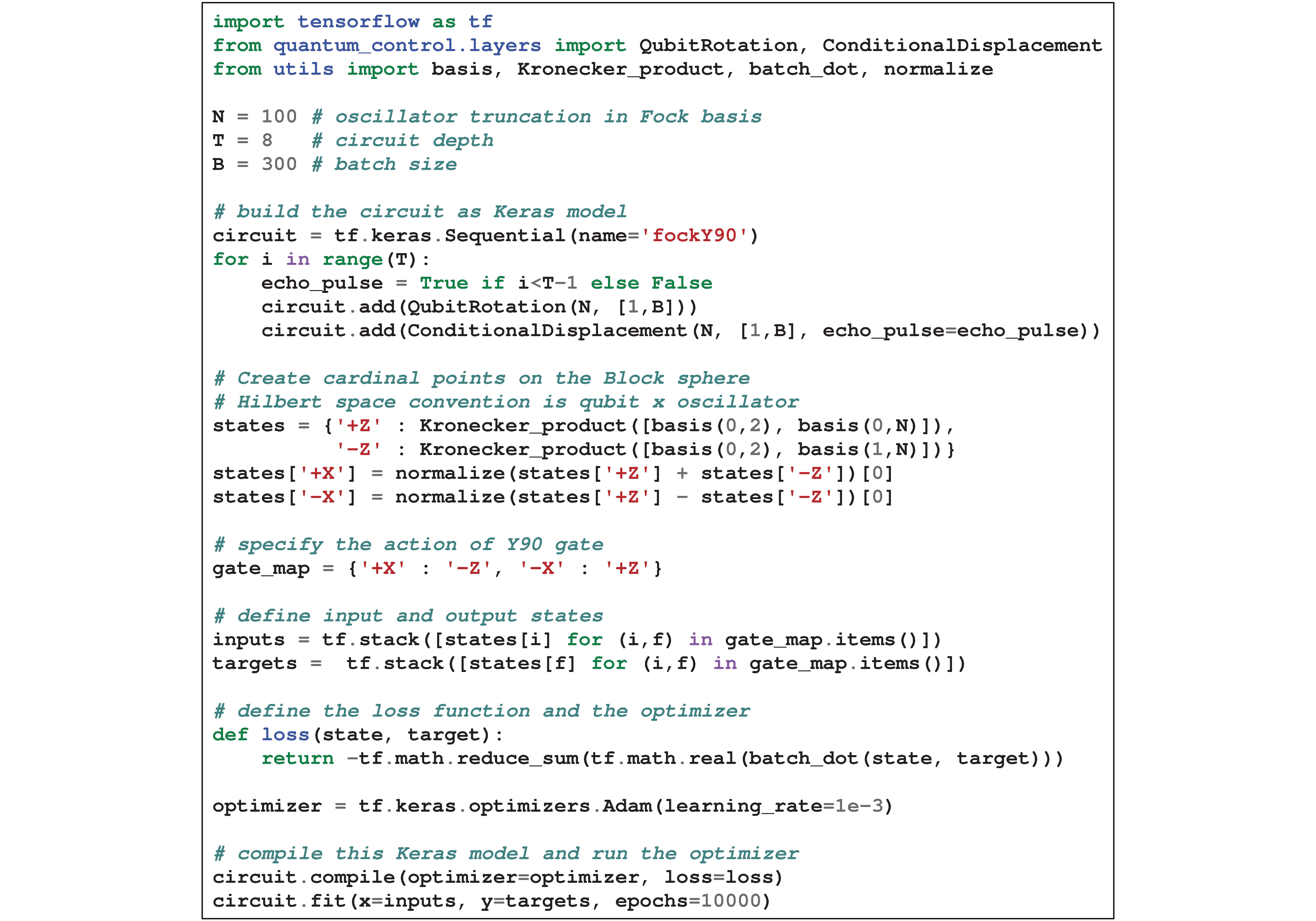
Circuit optimization. A circuit optimization method for this gate set was developed in Ref. Eickbusch et al. 2021. Here, we present a simplified modular framework based on the Keras library Cho, which allows to optimize circuit parameters in a manner similar to training of the neural networks. The parametrized control circuits (S13) are created as instances of the tf.keras.Sequential class which is commonly used to concatenate multiple neural network layers. Here, we instead use custom layers that represent the parametrized gates and as subclasses of tf.keras.layers.Layer. This allows us to exploit flexible and user-friendly application-programming interface of the Keras library to optimize the circuit parameters and automatically monitor various aspects of the optimization progress. To illustrate the accessibility of such an approach, in Fig. S9 we provide an example code for optimization of the gate on the qubit. Complete code with dependencies and further examples is available in Ref. Siv. Such optimization, which is performed for a batch of circuit candidates in parallel on a graphics processing unit (GPU), takes about minutes to finish. In Table S2, we list circuit parameters for some of the control operations in our experiment. Curiously, some of the numerically optimized parameter values are clearly interpretable, e.g. in GKP state preparation circuit the rotations at steps seem to be by an angle . Detailed inspection of these circuits can lead to improved analytic constructions, which is left for future research.
Pulse compilation. Having obtained the circuit parameters, we compile the waveforms to be played on the qubit and oscillator control lines. Such compilation requires prior calibration of the rotation gate, described in Section S2.1, and the gate, described in Section S2.4.
As explained in Ref. Eickbusch et al. 2021 and in Section S2.4, our experimental implementation of the gate results in additional qubit phase accumulation , i.e. we implement . We use the experimental calibration of this phase to adjust the numerically optimized vector according to the rule
| (S14) |
In addition, in many cases of interest the ancilla qubit at the end of the circuit returns to and disentangles from the oscillator. In such cases, the last conditional displacement can be realized as a simple displacement . We use this simplification in state preparation circuits and in the SBS protocol.
In Fig. S10, we show an example waveform for unitary preparation of the grid state using a parametrized circuit with layers. Each gate is decomposed via large displacements and conditional rotations. For clarity, in this example all conditional rotations are implemented with a constant wait time ; hence, the whole compiled waveform has a duration of . Faster implementations are possible if the wait time is adapted to the magnitude of the conditional displacement, as described in Section S2.4. For example, in our system the conditional displacement of amplitude could, in principle, be implemented with zero wait time, see Fig. S6(d).


S3.2 Model-free reinforcement learning for QEC
While most quantum operations in our experiment are optimized with a model-based approach described above, for quantum error correction we deploy a more powerful framework of model-free optimization. We use a reinforcement learning algorithm called proximal policy optimization (PPO) Schulman et al. 2017; Guadarrama et al. 2018. For a detailed description of this algorithm in the context of quantum control we refer to Ref. Sivak et al. 2022; here, we only provide a basic high-level picture. The complete training loop of our experiment is illustrated in Fig. S11; it is structured as follows:
Step 1. On training epoch , neural network produces a probability distribution , where , , and summarizes the values of all weights and biases of the neural network in the current epoch.
Step 2. We sample a batch of parameter vectors from this distribution. They correspond to different QEC circuit candidates that should be evaluated in experiment. The neural network and sampling are implemented on NVIDIA 2080Ti graphics processing unit (GPU) in a separate computer. The sampled vectors are sent to the control computer via a local area network with negligible communication time.
Step 3. Based on these parameter vectors, we compile QEC circuit candidates, translated into FPGA instructions and DAC waveforms. All circuit candidates follow the same program execution flow, but the control waveforms and the content of FPGA registers is different for every candidate. The FPGA is reset and its wave memory is updated. This time-consuming step is the bottleneck of the training loop.
Step 4. Each candidate is evaluated in experiment. To this end, we initialize logical Pauli eigenstates and , run the QEC for cycles, and then perform one-bit phase estimation of the corresponding logical Pauli operators. To suppress the sampling noise, we repeat this times per Pauli and per circuit candidate. In total, one epoch of training consists of experimental shots.
Step 5. To produce the reward, we treat the measurement of a Pauli operator after cycles as a proxy for logical lifetime. While averaging the measurement outcomes, we mask the experimental shots that started with incorrect state initialization, as flagged by a verification ancilla measurement after the state initialization.
Step 6. Once the rewards are available, PPO algorithm updates the neural network parameters for the next epoch. The gradients of these parameters are computed with automatic differentiation via back-propagation. After updating the neural network, the new training epoch begins.
The time budget of this training is shown in Fig. S11. All steps outlined above amount to per epoch. In the current implementation, the major bottleneck is Python-to-FPGA transition (step 3). Because of this, the implementation is less optimal in terms of sample efficiency than the proposal in Ref. Sivak et al. 2022. The optimal approach would be to spend the total sample budget per epoch to evaluate more circuit candidates with minimal accuracy, instead of evaluation only a few candidates with high accuracy (achieved through averaging). In other words, based on the results of Ref. Sivak et al. 2022, we expect that a training with would require fewer experimental shots to reach a given performance level than a training with . However, considering the total run time of the training, we had to compromise between bare sample efficiency (number of shots) and the overhead in step 3 of the pipeline. The overhead is independent of but increases with , and due to a limited FPGA instruction sequence length we can only evaluate candidates per compilation. After paying the compilation overhead in step 3, a certain amount of averaging comes essentially for free and does not considerably affect the run time, hence the choices made here.
In Section S4.4, we describe the QEC circuit parametrization, show the evolution of parameter values during the course of training, and provide interpretation of the observed trends.
S4 Quantum error correction of the grid code
S4.1 Brief introduction to grid code

Qubit-register stabilizer codes are based on the group of Pauli operators; consider instead a stabilizer code based on the group of oscillator displacement operators. By definition, the eigenstates of a displacement operator are displacement-invariant in phase space along the direction of with a period . Having two code stabilizers and imposes displacement invariance along two non-equivalent directions, which means that all codewords are grids in phase space with a unit cell defined by . The requirement of commutativity of and imposes a constraint
| (S15) |
where . Here, we consider encoding of a single logical qubit into an oscillator, which corresponds to . By parametrizing the complex-valued displacement amplitudes as and , we obtain a grid code with the following stabilizers:
| (S16) | ||||
| (S17) |
From the constraint (S15) we derive a single requirement that a real matrix has a determinant . This matrix defines the structure of the grid in phase space. Here, we only consider the square grid code, which is obtained with . The hexagonal code with was realized in Ref. Campagne-Ibarcq et al. 2020.
The Pauli operators of the logical qubit are defined as
| (S18) | ||||
| (S19) |
They satisfy the standard algebraic properties , , and , inside the code space. Using the identity , we find the third Pauli operator .
The eigenstates of Pauli of the ideal grid code are shown in Fig. S12(a). Finite-energy code families can be obtained by regularizing the ideal code through application of an envelope operator Tzitrin et al. 2020; Royer et al. 2020, with a common choice being . We show several members of this code family in Fig. S12(b-d). Note that such a regularization leads to non-orthogonal states, with fidelity loss due to the finite state overlap that scales as (see Eq. S28 in Ref. Royer et al. 2020), which is negligible for our choice of .
S4.2 Small-Big-Small (SBS) protocol

Here, we describe the SBS protocol, first proposed in Ref. Royer et al. 2020; de Neeve et al. 2022 from a new angle. The full QEC circuit in this protocol is shown in Fig. S13(a) with nominal parameter values listed in Table S2; it implements a channel . Let denote the Kraus operators of the constituent rank-2 channels (we omit the subscript from the Kraus operators for simplicity). These operators read:
| (S20) | ||||
| (S21) |
where and , and are obtained with a substitution . Then, the Kraus operators of a composite rank-4 channel are:
| (S22) |
For , these Kraus operators are shown as matrices in the truncated eigenbasis of in Fig. S13(b). This eigenbasis splits into pairs of states , , that define orthogonal replicas of the logical subspace generated by the errors. We show the Wigner functions of the projectors , , and onto the first three subspaces in Fig. S13(d). Note that and , hence the errors in the first level of hierarchy resemble photon loss () and gain () errors. While and only approximately satisfy the Knill-Laflamme conditions Knill and Laflamme 1997 for the finite-energy grid code, the actual error operators that define the subspaces and satisfy these conditions exactly (since the eigenspaces of a Hermitian operator are orthogonal). Similarly, by inspecting the Wigner functions of the projectors onto higher subspaces, we find that the second level of error hierarchy resembles , and . The number of error subspaces in each level is given by the number of unique combinations of an : two subspaces ( and ) in the first level, and three subspaces (, and ) in the second level, leading to the blocks of size and in the Kraus matrices in Fig. S13(b). Further understanding the structure of the error hierarchy is the subject of ongoing research.
Unlike in the standard stabilizer formalism of QEC Gottesman 1996, Kraus operators here do not correspond to a projection of a state onto a single error subspace and its subsequent transfer to the code space. Instead, the transfer here is realized gradually, following an error hierarchy imposed by the QEC circuit. To clarify the action of the Kraus operators, their reduced representation using directional flow of a quantum state between error subspaces is shown in Fig. S13(c) [this representation ignores the dynamics within each subspace]. We now briefly discuss the interpretation of the processes corresponding to each of the , , , outcomes of a QEC cycle. Outcome heralds a process in which the state has remained in the same subspace. The probability of emitting from within the code space is nearly . This property is exploited in Section S4.5 to extract the expectation value of the code projector from the statistics of long strings of the type. Both and outcomes herald the process in which the quantum state was transferred one level down the error hierarchy. Strings like therefore correspond to processes in which the state directionally hops level by level towards the code space. Finally, the outcome heralds a transfer two levels down the error hierarchy.
Besides the transfer between the error spaces, the Kraus operators apply a deterministic logical flip: in the cycles, and in the cycles. This flip is visible in the off-diagonal structure of the sub-blocks in the Kraus matrices, see Fig. S13(b). For example, the lower right block in represents the code subspace, and the off-diagonal structure represents the combined effect of on the codewords. Due to this effect, the lifetime of and logical Pauli eigenstates in our QEC protocol are exactly equal. We track the Pauli frame in software, and undo its change in the data reported in Fig. 3 of the main text.
To demonstrate how the errors are corrected by this QEC scheme, we show several examples of quantum state trajectories in Fig. S13(e). In the first trajectory, the state is initialized as one of the logical basis states, and then evolved for several QEC cycles without any errors. The Pauli frame switching is apparent here from the oscillating pattern within the code space (in this picture, the phase information is not shown, but the QEC process also protects the phase of the logical qubit). In the second trajectory, an error was applied to the state prior to QEC, and then it was almost perfectly corrected, accompanied by the emission of syndrome string. In the third trajectory, this error was instead corrected during the third QEC cycle, and the quantum state spent extra time in the error space . This example explicitly demonstrates that the Pauli frame update is applied correctly irrespective of the subspace, hence Pauli gates done in this manner are transversal. The subsequent trajectories demonstrate that even higher-order errors, such as or , can be corrected with high fidelity. Moreover, as seen in the fifth trajectory, the state can be recovered even if additional errors happen while the previous errors have not yet been fully corrected. The latter example highlights that the “slowness” of the low-rank error-correction dissipation is not a problem, as long as the error rate is sufficiently small compared to the correction rate.
A few remarks with regards to the simplified interpretation of the QEC process in the main text are in order: (i) The correct interpretation of the action of a QEC cycle requires considering pairs of outcomes, like , instead of isolated outcomes, like or . We adopted the latter approach in the main text for simplicity of exposition. (ii) The outcome does not herald the projection onto the code space, as mentioned in the main text, but rather a process in which “no error was corrected”. Conditioned on the state residing in the code subspace, this outcome will be emitted with probability nearly 1. However, if the state is in one of the error spaces this outcome can still occur with smaller probability starting from about at the lowest level in the error hierarchy and reducing for higher levels. (iii) When one of the outcome , or is obtained, there is a small chance that the QEC process has added an error, leading to a random walk among the error spaces that is heavily biased towards the code space.
S4.3 QEC cycle: implementation details
In this section, we describe implementation details of a QEC cycle, whose schematic is shown in Fig. S13. The various datasets in this work were taken with several different versions of the QEC circuit. All these versions have the same overall structure, but different parameter values obtained from re-training after the system drift has appreciably affected the logical performance (this happens on a time scale of 1-2 weeks, see Section S4.10). Below, the quoted durations of various components of a QEC cycle refer to the circuit version that we used to collect the system lifetimes dataset and that achieved the highest reported QEC gain.
SBS unitary. We refer to the unitary part of the circuit prior to ancilla measurement as “SBS unitary” since it is based on the ansatz from Ref. Royer et al. 2020. The SBS unitary is compiled as a four-layer parametrized circuit with nominal parameters shown in Table S2, and is further translated into the pulse sequence with the method described in Section S3.1. The last circuit layer does not contain an gate, and instead only contains a qubit rotation and oscillator displacement. Since the qubit is reset after the SBS, the function of the latter rotation is to choose the “reset axis”, which can be an arbitrary axis on the qubit Bloch sphere.
As shown in Ref. Royer et al. 2020, without any special asymmetries between and it would not matter along which axis the ancilla reset is done – all choices result in the same completely positive trace-preserving map after averaging over the measurement outcomes. However, in practice the asymmetry comes from the ancilla relaxation channel that degrades the readout fidelity of the state. Hence, it is advantageous to choose the reset axis that preferentially returns the outcome. The parameter sequence for SBS unitary in Table S2 takes this choice into account. The choice of reset axis also results in different unraveling of state trajectories and different Kraus operators. The choice made here enabled the interpretation of outcomes as syndromes that signal occurrence and correction of errors, which is utilized in the post-selection experiments, described in Section S4.7. This is in contrast with Ref. Campagne-Ibarcq et al. 2020, where and outcomes are interpreted as left or right displacement of the grid.
The duration of the SBS unitary is not fixed, because its constituent gates can be implemented with different choices of the speed enhancement factor (amplitude of the intermediate displacement). Since is included in the action space of the RL agent, all circuit candidates during the training have different durations of the SBS unitary (we will soon comment on how this affects the reward comparison among them). In the final circuit that achieved the highest reported QEC gain, the duration of SBS unitary is .
| Component | Subcomponent | Duration (ns) |
|---|---|---|
| Enter cycle | 24 | |
| SBS | Enter SBS | 24 |
| Circuit layer 1 | 502 | |
| Circuit layer 2 | 708 | |
| Circuit layer 3 | 262 | |
| Circuit layer 4 | 76 | |
| Exit SBS | 24 | |
| Reset | Enter reset | 24 |
| Roundtrip delay | 300 | |
| Acquisition | 1400 | |
| Signal processing | 332 | |
| Distribution of and | 100 | |
| Branching and feedback | 200 | |
| Exit reset | 24 | |
| Virtual rotation | Mixer matrix calculation | 400 |
| Mixer update | 48 | |
| Idle | Delay | 452 |
| Exit cycle | 24 |
Ancilla reset. In principle, error correction with SBS protocol could be fully autonomous (without a classical feedback loop) as was envisioned in the proposal Royer et al. 2020 and realized in a trapped ion system de Neeve et al. 2022. The autonomous scheme has an advantage of significantly simplifying the demands on the classical co-processor (in our case, the FPGA). Moreover, there exist various dissipative reset protocols for the transmon Murch et al. 2012; Geerlings et al. 2013; Magnard et al. 2018. However, the disadvantage of a fully autonomous implementation in our system is that it is not able to compensate for a spurious rotation of the oscillator due to the always-on dispersive coupling with the ancilla. The back-action of discarding the ancilla state during the reset is the dephasing of the oscillator – a particularly harmful error channel for the GKP code Royer et al. 2020. Partly because of this reason, we chose to implement ancilla reset through measurement and classical feedback, as described in Section S2.3, with the total duration of ancilla reset subroutine of .
Virtual rotation. Due to the always-on dispersive coupling, the oscillator acquires a spurious rotation during the ancilla readout time. In experiment Campagne-Ibarcq et al. 2020, a simple echo sequence was used to cancel this rotation. With such an approach, ancilla spends half of the time in and half in regardless of the actual syndrome measurement outcome, which is detrimental to the code due to additional error sources associated with the state. Here, we instead chose the reset axis which results in probability of detecting . Therefore, the ability to compensate for the spurious oscillator rotation without echoing the state back to is crucial to maintain this advantage.
We achieve this by dynamically tracking the oscillator phase that stochastically changes due to random ancilla measurement outcomes, and compensating for it with a virtual counter-rotation. The spurious oscillator rotation angle accumulates during the reset time , during the time that it takes to execute the virtual rotation on the FPGA, and during the idle time when ancilla is nominally in (the latter will be explained shortly). Therefore, in the idealistic dispersive coupling model, the oscillator would rotate by if the ancilla is found in , and if it is found in . Although the state is not computational, our controller is able to reset it with an accompanying virtual rotation by angle . Instead of relying on the simple dispersive coupling model, in experiment we independently calibrate the angles with a variation of out-and-back experiment Eickbusch et al. 2021 to account for additional minor timing contributions related to FPGA program entering or exiting a subroutine, etc. These calibrated angles are used to initialize the QEC circuit for training.
Another important aspect of the virtual rotation is the switching between momentum and position quadratures of the oscillator to realize and dissipators. Such switching can be achieved with a rotation of the SBS unitary by in phase space. This results in additional deterministic contribution in every virtual rotation gate. The value of is for the square grid code, and for hexagonal grid code.
The virtual rotation gate utilizes a floating point register on the FPGA. During this gate, the FPGA performs the calculation with subsequent reconfiguration of the dynamic mixer matrix which applies a rotation transformation to the oscillator pulses before they are being streamed at the DAC. The total duration of the virtual rotation gate that includes all these steps is independent of and is equal to .
Idle section. During the agent training, the reward is measured after a fixed number of cycles, and not after some fixed physical duration of time. Therefore, it is necessary to keep the duration of a QEC cycle constant across different protocol candidates to ensure a fair reward comparison. At the same time, the agent is able to affect the physical duration of the SBS unitary by changing the speed enhancement factor in the gates. To reconcile these two requirements, after the virtual rotation gate we add a section of idle time that is calculated based on the duration of the SBS unitary in each circuit candidate. We constrain the combined duration of SBS unitary and the idle section to be . In the circuit that achieved the highest reported QEC gain, the duration of the idle section was . Note that in the previous QEC experiments that tried to create a long-lived quantum memory Ofek et al. 2016; Hu et al. 2019, the idle section was inserted intentionally to avoid frequently entangling the high-quality oscillator with low-quality ancilla. Here, we find that inserting any additional idle time degrades the performance, hence we kept it nearly to a minimum while still leaving some room for change of the SBS duration by the RL agent.
In Table S3, we provide a detailed timing breakdown of all components of the cycle.
S4.4 Learned and scripted parameters

Our QEC protocol has multiple parameters which could be optimized to improve its performance. Some of these parameters are difficult to incorporate into our optimization framework in its current form, and therefore their values are chosen as an approximate compromise between various tradeoffs and then held constant. The rest of them are optimized with reinforcement learning, given a reasonable starting point obtained from independent calibrations. Here, we briefly explain the meaning of these parameters.
Scripted parameters:
Duration, shape, and amplitude of the readout pulse.
State classification thresholds.
Timing of all components of the reset subroutine.
Durations of primitive pulses (qubit rotations and oscillator displacements).
Combined duration of the SBS unitary and the idle section.
Learned parameters:
Virtual rotation angle for each measurement outcome. It is initialized with a result of independent calibration using a variation of out-and-back experiment.
Detuning of transmon and pulses (same parameter for all pulses). It is initialized with a result of independent calibration, when oscillator is in the vacuum state (i.e. when there is no Stark shift).
Spectral corrections to and pulses based on derivative reduction by adiabatic gate (DRAG) scheme Chen et al. 2016 (same parameter for all pulses). It is initialized with 0.
Complex-valued amplitudes of conditional displacement gates in the first three layers of the SBS unitary, and a complex-valued amplitude of the unconditional displacement in the fourth layer. Two small amplitudes are initialized with , and the big amplitude is initialized with . The unconditional displacement is initialized with 0.
Magnitudes of the intermediate large displacements used to execute the gates in the first three layers of the SBS unitary. They are initialized with for small conditional displacements and for the big conditional displacement. Note that changing these parameters also influences the duration of the gates.
Angular corrections to intermediate large displacements in the first three layers of the SBS unitary. These heuristic parameters compensate for effect of second-order dispersive shift and for the fact that conditional displacement accumulates along an arc of small curvature instead of a straight line. These corrections are initialized with 0.
Phases and angles of all ancilla rotations in the SBS circuit layers (including the echo pulses inside the gates), and in the ancilla reset subroutine. These parameters are initialized with nominal values from Table S2.
Detuning of the local oscillator (LO) frequency for the cavity mode. This LO is calibrated with spectroscopy and set to be half-way between the number-split oscillator frequencies when qubit is in the states and , corresponding to in Eq. (S1).
Evolution of parameters during training. In Fig. S14, we show the evolution of several QEC circuit parameters during the training. Most parameters, when initialized well, merely exhibit small fluctuations around the mean. However, some parameters undergo systematic and reproducible changes, as observed in the provided examples. For instance, in Fig. S14(a), the big conditional displacement amplitude , which we expect to be equal to the size of the grid unit cell, changes from a calibrated value of by about , likely indicating the presence of a miscalibration error (the last calibration was done several weeks prior to this training). Similarly, the trend in Fig. S14(e) towards the negative detuning of the pulses could be compensating for an additional Stark shift that was not present at the initial calibration stage (calibration was performed with vacuum state in the oscillator). In Fig. S14(b), the trend in amplitudes and of the two small conditional displacements in the SBS unitary is particularly insightful, as it helped us identify a limitation of the proposal in Ref. Royer et al. 2020, according to which the amplitudes and should be identical and equal to , while the RL agent systematically converges to . Using simulations, we verified that in presence of error channels that act during the execution of the SBS unitary, this is indeed a correct inequality. The optimal ratio of these two amplitudes is found in simulations to be strongly dependent on the error channel. The agent adapts this ratio to the real error channel of our system.
In Ref. Sivak et al. 2022, it was shown that a similar RL agent is able to converge to correct solutions even starting from completely random parameter initializations. Here, we initialize the parameters close to their expected optimal values through various calibrations, but the compounded effect of small errors (at the level of a few percent) in multiple parameters results in a QEC protocol which, although fully functional, is far from optimal. In particular, we were not able to reach break-even with only the independent calibrations and educated guesses, hence model-free RL can be acknowledged as one of the most crucial factors in the success of this project.
S4.5 Syndrome measurement statistics


A sample of experimental QEC shots is shown in Fig. S15, where QEC is ran for cycles in each shot. Consider a string of measurement outcomes going from any chosen time step to a time step (it contains QEC cycles). The probability that this string contains only outcomes is shown in Fig. S16(a), where it is averaged over the experimental shots and over initial times (the averaging over is done with a sliding window method which is applicable due to process stationarity). While in the most general case the functional form of is a sum of multiple decaying exponentials, we clearly observe only a single dominant exponential contribution. Hence, we fit this probability to , obtaining and . By adopting a model for the error process and for the QEC process, we can link the fit parameters to model parameters. In general, such a model would be quite complex. However, here we are interested in only two characteristic parameters of the process: the probability of occupying the code space in the dynamical equilibrium of the QEC process, and the probability of having an error that transfers the state out of the code space. These parameters can be extracted with very minimal model assumptions.
Using the transfer matrix approach, it can be shown that and under the following assumptions: 1) The error probability is small , which is justified since the cycle duration is small compared to all relevant error rates in the system, and is confirmed by the fit results; 2) The conditional probability of emitting when the quantum state is in the code space is nearly 1. This is justified, since in the error-free model of the SBS protocol described in Section S4.2 this probability is ; 3) The conditional probability of emitting when the quantum state is in any of the error spaces is small . This assumption is partially justified, since in the error-free model of the SBS protocol this probability is smaller than for the first error space, and then monotonously reduces for the higher levels of the error hierarchy; 4) The probability of correcting an error and emitting is small . In the error-free model of the SBS protocol this probability is exactly zero, while in practice it is limited to due to the readout infidelity of the state.
This result can be intuitively understood as follows: the two most probable system trajectories that generate the string of all ’s correspond to (i) starting in the code space and remaining there for steps, which happens with probability , and (ii) starting in the code space, remaining there for steps, and transitioning out on the very last step, which happens with probability . The sum of these two contributions equals , leading to and . The corrections to these formulas are of the second order in parameters . From the fit in Fig. S16(b), we extract and . Note that this result for agrees within the error margin with the result obtained by an independent method based on the reconstruction of the density matrix from the measured Wigner functions in Section S4.8. Here, the error of the fit is negligible compared to the model approximations, hence the quoted error bars are obtained from an estimate of the second-order corrections .
Here, we only considered the string of a special type ; an important avenue of future research would include learning the error channel from the full statistics of syndrome outcomes, using the dataset in Fig. S15.

S4.6 Analysis of transmon leakage
To quantify transmon leakage, we histogram its duration in Fig. S16(b). The most likely leakage duration is cycle, since the controller resets to with high probability. However, because of the finite readout fidelity of , shown in Fig. S5(b), the controller sometimes fails to reset this state, resulting in the next most probable leakage duration of cycles. After that, the histogram follows exponential distribution with decay constant of cycles, corresponding to , which we attribute to the effective lifetime of higher leakage states that are not addressed by our reset scheme. This time scale is consistent with our estimate of the state lifetime, derived from the bosonic statistics and the average measured lifetime of state.
To extract the leakage rate, in Fig. S16(c) we plot the fraction of shots that experienced a leakage event of a certain duration up to a given cycle. We fit the data to a constant-rate model where is the cycle index and is the leakage rate (i.e. leakage probability per cycle). We find cycles, corresponding to a leakage rate of . Similar analysis can be done for leakage events of length ; with the fit to the same model, we find the time scale of cycles, and the corresponding rate of . Note that this measurement was performed at the time of slightly sub-optimal performance, and therefore the leakage rate at the maximal achieved QEC gain might have been smaller.
Next, we study the correlation of syndrome measurement outcomes across time. The correlation matrix is given by
| (S23) |
where is the measurement outcome obtained at cycle , and empirical expectation values are obtained by averaging across experimental shots. For the dataset of Fig. S15 this correlation matrix is shown in Fig. S17(a), where we consider only the first cycles. Overall, the correlation is weak, and the correlation between and channels (separated by odd number of cycles) is weaker than the correlation between the same-quadrature channels (separated by even number of cycles).
By zooming in the color scale to visually resolve small numbers and considering the full duration of the trajectory of cycles, as shown in Fig. S17(b), it becomes evident that the process is not perfectly stationary. To emphasize this, we show in Fig. S17(d) the correlation coefficient as a function of for several choices of . Further along the QEC trajectory the process acquires a correlation tail. Although quite weak, this correlation stretches over hundreds of cycles.
Previously, it was demonstrated that leakage removal helps to reduce correlated errors in the arrays of transmons McEwen et al. 2021. Our QEC protocol already contains a mechanism for leakage removal from the state through measurement-based feedback in every cycle. However, leakage states higher than are not cleared by our reset. The signature of such leakage events to higher states is two or more consecutive leakage syndrome outcomes. To check the hypothesis that this residual leakage to states higher than is responsible for increase of correlation, we post-select trajectories that do not have any length-two or longer leakage events. In the post-selected dataset, the correlation matrix does not display any detectable non-stationarity, as seen in Fig. S17(c,e), confirming the hypothesis. By fitting the remaining short-time correlations in Fig. S17(e) to an exponential decay, we conclude that it takes cycles (approximately 2 QEC cycles) to lose the memory of a typical large error. However, the most probable small errors are corrected in a single QEC cycle.
| NP | L | ||||||||
|---|---|---|---|---|---|---|---|---|---|
|
|||||||||
|
|||||||||
|
|||||||||
|
|||||||||
|
|||||||||
|
S4.7 Post-selection of errors
Here, we provide additional details about the the post-selection experiment that verifies the ability of our QEC scheme to faithfully identify the errors. The post-selection results are summarized in Table S4. Note that this experiment was performed at the time of slightly sub-optimal system performance, hence the baseline results with no post-selection are lower than in some other experiments reported here, e.g. in Section S4.10. The main conclusion of this post-selection experiment is that it enables significant improvement of the error probability at a cost of only a modest rejection probability.
The saturation of lifetimes in the most stringent post-selection scheme (which preserves only the all- trajectories) can be related to the following mechanisms: (i) Direct logical errors, which are undetectable in any QEC scheme. (ii) Misclassification of as (due to ancilla decay during the measurement), which means that some of the all- trajectories that survived the post-selection actually contained errors, and some of those errors might have been close to a logical operation instead of the identity operation. (iii) The non-orthogonality of logical states, which in our case is not a limiting factor.

S4.8 Wigner tomography of logical states
Tomography and its calibration. Wigner tomography is derived from the expression for the Wigner function , where is the displaced parity operator, and is the photon number parity. The displaced parity operator is unitary and can be measured with phase estimation. It is also hermitian, and hence its eigenvalues are constrained to be . Therefore, it is particularly convenient to measure displaced parity by mapping it onto the qubit observable Vlastakis et al. 2013, which is achieved in our system with a circuit shown in Fig. S18(a). The conditional rotation gate is realized with a delay of duration under the dispersive coupling Hamiltonian, which amounts to approximately . Because of such long duration, previous GKP experiments with similarly small chose to perform state tomography using the characteristic function instead Campagne-Ibarcq et al. 2020; Eickbusch et al. 2021. However, the long coherence of our system allows to measure Wigner function with reasonably high fidelity.
We use several calibration techniques to improve the quality of the subsequent state reconstruction from the tomographic data. First, to symmetrize the effect of ancilla relaxation during the readout, in half of the phase estimation runs we map eigenvalue of to the outcome, and in another half to the outcome. This technique eliminates any finite offset in , but maintains reduced contrast due to ancilla relaxation and decoherence. Next, to calibrate the contrast reduction, we perform an experiment with a similar circuit in which is replaced with , see Fig. S18(b). We fit the result of this experiment, shown in Fig. S18(c), to , where is the purity loss per gate. Under the assumption that contrast reduction in tomography is primarily due to incoherent processes (ancilla relaxation and dephasing, and oscillator photon loss), the inferred tomography contrast is . At , this inferred contrast is equal to , which matches the measured contrast of the Wigner function of vacuum in Fig. S3(c), justifying the assumptions of this calibration method.
The phase space points for Wigner tomography are chosen on a square grid in a complex plane restricted to . We acquire shots per point in separate acquisition time frames. Between the time frames we perform system performance checks; data acquisition is put on hold if the spurious resonance in reappears [see Fig. S5(d)]. A single state tomography dataset consists of million shots, and takes a long time to acquire – from hours in the case of cycles, to hours in the case of cycles. Therefore, conclusions derived from the analysis of tomography data apply to long-time average system performance.
State reconstruction. Tomographic data is used to produce a best guess for the density matrix of the state. We parametrize the density matrix as , where , and and are real-valued matrices. Such parametrization ensures that is positive semi-definite with trace 1. We truncate the density matrix to dimension in photon number basis. Coefficients of matrices and are optimized using the least squares fit of the Wigner tomography and contrast data, with the cost function given by
| (S24) |
An example Wigner tomography of the grid state together with its reconstruction is shown in Fig. S18(d-f). As will be described shortly, using the reconstructed density matrix we extract various parameters of the state: its purity, mean photon number, and envelope size.
Evolution of logical states. We visualize the evolution of logical and grid states during the QEC by taking Wigner tomography snapshots after , , , , and cycles, with results shown in Fig. S19.
The marginal of the Wigner function along momentum quadrature gives the probability density of the oscillator position, shown in the third row of Fig. S19. The and states have non-overlapping support in position representation, clearly observed in the data at cycles. During the QEC process these basis states mix under the logical Pauli channel, which is manifested in the appearance of position peaks of the opposite state, until finally they become almost (but not completely) indistinguishable after cycles.
On the other hand, the marginal of the Wigner function along position quadrature gives the probability density of the oscillator momentum, shown in the last row of Fig. S19. In the momentum representation, and states share the same support, but have a different pattern of phases associated with the peaks of the wavefunction. The phase information is discarded in the probability density function, which looks identical for both states.

Spectral analysis of reconstructed states. Focusing on the time evolution of the state, we perform spectral decomposition of its reconstructed density matrices at . We find that the eigenvalues of the density matrix are arranged in pairs corresponding to the images of this state and of its complement in different subspaces of the QEC, see Fig. S20(a). In particular, we identify only two subspaces with a substantial presence of the state during the QEC process: the code space , shown in Fig. S20(b), and the error space corresponding to an error that most closely resembles , see Fig. S20(c) and Section S4.2.
While the QEC circuit imposes the structure of the error subspaces, as described in Section S4.2, the properties of the “thermal” distribution across these subspaces in the dynamical equilibrium is defined by the strength of the various error mechanisms in our system as well as the rate at which these errors are corrected. The probability of occupying the code space, given by the sum of the first two eigenvalues, remains constant over time and equal to , where error bar represents the standard deviation with respect to different durations of the QEC process. This value agrees well with an independent analysis in Section S4.5. Having only one relevant error subspace in the steady-state distribution also qualitatively agrees with an observation in Section S4.5 that errors are rare. We believe that other error subspaces are populated with probability , which is beyond the resolution power of this method. Developing a more accurate and sample-efficient reconstruction technique for characterizing the distribution across the error spaces is an important direction left for the future.

Extracting code envelope size. For each QEC duration , the reconstructed density matrix is used to find the fidelity of the experimental states to the family of finite-energy codewords parametrized by the envelope size . For , we additionally displace the target codewords by to account for a small shift visible in the tomography. Since these target states are pure, the fidelity is given by and . For experiments that start with a preparation of , these fidelities are shown in Fig. S21(a) for each QEC duration from the dataset in Fig. S19. Immediately after the initialization, the fidelity is maximized for , where it reaches . During the QEC process, gradually reduces while increases, consistent with the logical Pauli channel. The sum , which is equal to the expectation value of the code projector, remains nearly constant for . It is maximized at (), where it is equal to . This value is close to extracted from the density matrix spectrum, which indicates that the code stabilized in the experiment is indeed the one defined by the envelope operator with .
The purity of state is shown in Fig. S21(b). During the QEC process, it reduces below , since the steady state contains a mixture of the codewords with their images in the error spaces. However, the part of this mixed state that resides within the code space should approach a purity of . To confirm that this is the case, for every state we define its projection onto the code space as , where we only consider the code with the optimal envelope . As seen in Fig. S21(b), the purity of after initialization is close to , and after hundreds of cycles it approaches , as expected for the logical Pauli channel.
Lastly, in Fig. S21(c) we plot the evolution of the average photon number during the QEC process. The extracted steady-state photon number is .
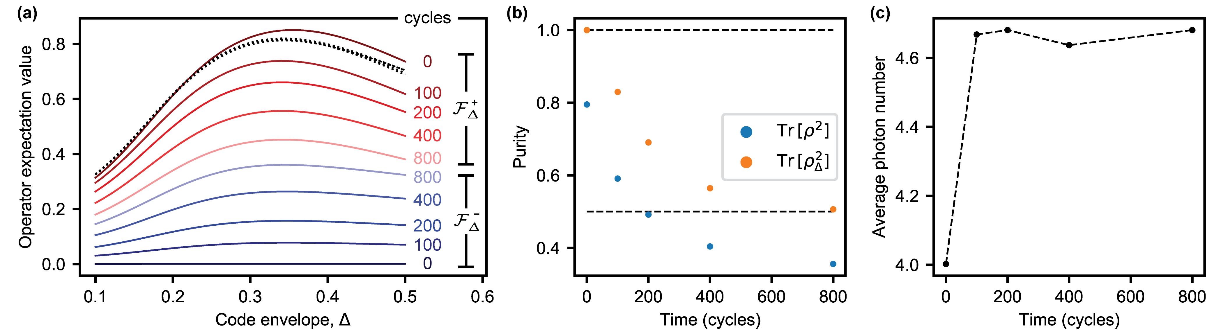
S4.9 Sensitivity to ancilla errors
Ancilla phase flips. Our QEC circuit is fault-tolerant with respect to ancilla phase flips by design Royer et al. 2020. To see this, consider that if error happens during the ancilla readout, it would have no effect because the readout projects the ancilla onto an eigenstate of . Likewise, during the virtual rotation gate or the idle time the ancilla is nominally in the state, which is an eigenstate of . Finally, the effect of errors on the SBS unitary can be understood by propagating them through the circuit layers. For example, if such an error happens during the big conditional displacement, it is equivalent to changing the circuit parameters from to . Since , this change is equivalent to a small error that will be corrected in the following QEC cycles.
Ancilla bit flips. In contrast, ancilla bit flips can detrimentally affect the logical qubit in several ways. If such an error happens during the middle half of the big conditional displacement of amplitude , it will with high probability generate a logical error. This mechanism accounts for a significant fraction of logical errors in the experiment. For example, its contribution to the Pauli error probability (per QEC cycle), is estimated to be , where the factors of account for (i) half of the superposition state being sensitive to ancilla decay, (ii) half of the QEC cycle is devoted to position quadrature, (iii) half of the big conditional displacement gate. In practice, the relaxation time of the ancilla is likely degraded during the execution of the conditional displacement due to the large number of intermediate photons in the oscillator, see Eickbusch et al. 2021 and evidence in Section S4.10. Hence, this estimate provides an optimistic lower bound. Ancilla bit flips can also create detrimental back-action on the oscillator if they happen during the readout time. Since readout outcome is used in a feedback loop to implement a virtual rotation gate, misclassification of the ancilla state generates rotational errors that the GKP code is not well suited to correct, with erroneous rotation angle distributed in the range radians. To estimate the contribution of such errors to the logical error rate, consider that a rotation by radians would diminish the overlap of the blobs in the Wigner function; therefore, a significant fraction of misclassification-induced rotation errors cause large disturbance of the stabilized code space. The transmon state is the most prone to misclassification. Since readout fidelity of the state is close to , and this outcome is generated of the time, we estimate an additional contribution to logical error probability per QEC cycle from this mechanism. The two contributions described here account for half of the logical error probability , and the remaining half is not yet well understood.
Transmon noise injection. To check the effect of ancilla errors on the logical performance in a controllable way, we perform noise injection experiments that selectively increase the transmon phase-flip rate or bit-flip rate , with the results shown in Fig. S22. With noise injection, we are able to increase by a factor of (spoiling from to ), and by a factor of (spoiling from to ). Using linear fits in the low-error region, we extract the error sensitivities , , , and . The derived sensitivity of to ancilla phase flips is 65 times smaller than the sensitivity to ancilla bit flips, confirming the qualitative arguments provided above. Mitigating the effect of ancilla bit flips on the logical performance is one of the most important future directions in grid-code QEC.
Verifying noise injection. In the following, we explain how the noise injection experiments were conducted and how we verified that the noise affects the system as intended, i.e. selectively tunes or . We are able to achieve high degree of selectivity, with negligibly small spurious effects. To spoil , we inject noise at the transmon frequency, and to spoil , we inject noise at low frequency Clerk et al. 2010. The baseband white noise with flat spectral density up to is sourced from an Agilent 33250A arbitrary waveform generator. In the tuning experiment, it is upconverted to the qubit frequency using a double-balanced mixer with an LO blue-detuned by from the qubit frequency. After this pre-processing, the noise is filtered and combined with the qubit control line after the switch (in contrast to all control pulses, the noise is not gated).
In Fig. S23(a), we inject resonant noise to tune . This noise couples to the operator and therefore changes and symmetrically, which results in increased steady-state population of the qubit, approaching at the largest applied noise power. Note that this noise also affects the dephasing rate , but the changes in are explained by changes in : the extracted pure dephasing rate remains independent of the noise power, as intended in this experiment. The error bars on increase at large noise power, because this small rate is extracted as a difference of two large rates. The oscillator dephasing rate is also affected by the noise, which is explained by the increased rate of qubit up- and down-transitions that dephase the oscillator through the dispersive coupling Reagor et al. 2016. The pure dephasing rate of the oscillator agrees reasonably well with the prediction derived from this mechanism (black dotted line). The disagreement at high noise power is under investigation; it likely comes from the breakdown of the simple formula for in the limit where is not small.
In Fig. S23(b), we inject baseband noise to tune . In addition to this desired effect, within the same dynamic range of the noise we observe an undesired increase of the qubit excited state population by a factor of (data not shown), likely due to the heating of the attenuators by the dissipated noise power. Since , the qubit lifetime is not significantly affected by this heating. The lifetime and coherence of the oscillator also remain independent of the noise power. The increase of the error bars on and with the noise power is related to strong degradation of the fidelity of the transmon selective pulse used to read out the population of the oscillator and states as described in Section S2.5. This pulse has a duration of and it is directly sensitive to the transmon coherence; at the highest injected noise power, where coherence time is spoiled down to , the fidelity of this selective pulse is only a few percent.
In Fig. S23(c), we show the effect of the noise on the readout fidelity of the transmon and states. In principle, the noise that induces phase flips ( errors) should not affect the readout of . However, due to the aforementioned heating of the qubit, we observe a weak degradation of . On the other hand, noise at the qubit frequency couples to and results in significant degradation of both and .


S4.10 Long-time system stability
With repetitive measurements of the lifetimes of qubit, qubit, and error-corrected GKP qubit, we investigate the stability of our quantum system over time, with results of a week-long scan shown in Fig. S24. We find that the qubit is the most stable, which we attribute to the fact that most of the electromagnetic field is stored in the vacuum of the cavity. In contrast, the qubit exhibits notable fluctuations of the state lifetime; such fluctuations are often observed in transmons Klimov et al. 2018; Carroll et al. 2021, and are typically attributed to two-level defects in the amorphous dielectric, although there are other mechanisms that could lead to such fluctuations, and their source in our system is not yet understood.
We also find significant fluctuations of the lifetime of an error-corrected GKP qubit. Periods of relative stability are regularly interrupted with sudden drops and resurgences of performance, correlated with the appearance and disappearance of a resonant feature in the dependence, see Fig. S24(c). The behavior of readout infidelity of the state is also correlated with this feature, see Fig. S24(b). We find that the correlation coefficient between the logical error rate and the readout infidelity is . However, preliminary simulations indicate that degradation of the readout fidelity alone is not sufficient to explain the collapses of the logical performance. We therefore believe that the presence of the spurious resonance affects not only the readout fidelity, but also the fidelity of the SBS unitary.
A plausible causal chain is the following: 1) for unknown reason, the spurious degrees of freedom (defects) appear and disappear; 2) when the transmon transition frequency is resonant with the defect, their interaction strength is enhanced, which reduces the lifetime of the state; 3) during the readout, the transmon is Stark-shifted by the readout photons into resonance with the defects, which increases the probability of readout errors; 4) when the transmon state is misclassified, the virtual rotation gate is executed with an incorrect angle, inducing a phase-space rotation error on the oscillator; 5) during the conditional displacement gates, the transmon is also Stark-shifted into resonance with the defects by the intermediate photons of the cavity mode; 6) when transmon decay happens during the big conditional displacement gate, it has a significant chance of inducing a logical error. This proposed connection between spurious defects and fluctuations of the logical performance could be verified with detailed system-level simulations that take into account time-dependent Stark shift of the transmon and Stark-shift-dependent degradation of , which is left for the future analysis.
Apart from the stochastic fluctuations, we observe a systematic drift that warrants periodic retraining of the QEC circuit. This drift can be seen by comparing the initial and final data points of the scan in Fig. S24, where all the monitored physical error sources are similar in magnitude, but the logical lifetime is reduced in the final point as compared to the initial point. Due to this effect, the various datasets reported in our work were acquired with different version of the QEC circuit that were retrained every 1-2 weeks.

S4.11 Average channel fidelity
The average channel fidelity of a quantum channel to a target unitary channel is
| (S25) |
where the integral is over the uniform measure on the state space, normalized so that . Henceforth, we refer to this metric simply as fidelity.
To derive an equivalent but experimentally-compatible expression, we make use of the Pauli transfer matrix (PTM) representation of a channel , where are Pauli matrices. This representation has several useful properties, e.g. that composition of channels corresponds to a product of their PTMs Greenbaum 2015. In terms of the PTM, we have the following expression for fidelity:
| (S26) |
where is often called the entanglement fidelity.
To benchmark a quantum error correction channel, we compare it to an identity channel with . In this case, Eq. (S26) can be further simplified to
| (S27) |
where we made use of the identities for , and . The complete derivation of this formula starting from Eq. (S25) can be found in Ref. Nielsen 2002. In experiment, the right-hand side of Eq. (S27) is measured by preparing Pauli eigenstates, passing them through the channel , and then measuring the corresponding Pauli operator, as cartooned in Fig. S25(a). Such a procedure is applicable to an arbitrary duration of the channel .
We focus on the comparison of three different qubits in our system: , , and an error-corrected GKP qubit. The free evolution of the two passive qubits is modeled using a composite amplitude damping and white-noise dephasing channel, while the evolution of an error-corrected GKP qubit is modeled using a logical Pauli channel. Given these well-justified assumptions on the error channels, from Eq. (S27) we find:
| (S28) | ||||
| (S29) | ||||
| (S30) |
We show the time evolution of the fidelity given by Eqs. (S28S30) in Fig. S25(b), using experimentally extracted decay rates at the highest QEC gain measured in our experiment.
As seen above, in general the fidelity decays to its steady-state value in a way that cannot be characterized by a single time constant even in the simplest error models such as Pauli noise or amplitude damping. Therefore, fitting the fidelity decay to a single exponential is not strictly valid, although this heuristic approach was adopted in the previous works on bosonic QEC Ofek et al. 2016; Hu et al. 2019; Gertler et al. 2021. To avoid such an inconsistency, we consider the channel acting for only a short time . Any time dependence of the fidelity, even if it contains multiple exponentially decaying contributions, at short times is equivalent to a linear decay:
| (S31) |
where is an effective depolarization rate, and is the fidelity lifetime. For a depolarizing channel with a depolarization probability , we have , motivating the name and the coefficient in Eq. (S31). For qubits considered here, the effective depolarization rates are:
| (S32) |
We define the coherence gain as an improvement of the effective depolarization rate of an error-corrected logical qubit over the best physical qubit in the same system (with the break-even point corresponding to ). In a bosonic circuit QED system, the latter is typically the qubit, hence . The highest gain achieved in our experiment is . During a scan discussed in Section S4.10, gain remained above break-even of this week-long time window, with a median of .
Lastly, we acknowledge that the decay constant of the average channel fidelity is not the only relevant metric that we expect to be correlated with the future ability of such systems to participate in quantum computations. Other metrics, such as the SPAM fidelity and the fidelity of gates, are important as well, and we leave their optimization and detailed characterization for future work.

References
- Axline et al. (2016) C. Axline, M. Reagor, R. Heeres, P. Reinhold, C. Wang, K. Shain, W. Pfaff, Y. Chu, L. Frunzio, and R. J. Schoelkopf, An architecture for integrating planar and 3D cQED devices, Applied Physics Letters 109, 042601 (2016).
- Rosenblum et al. (2018) S. Rosenblum, P. Reinhold, M. Mirrahimi, L. Jiang, L. Frunzio, and R. J. Schoelkopf, Fault-tolerant detection of a quantum error, Science 361, 266 (2018).
- Place et al. (2021) A. P. Place, L. V. Rodgers, P. Mundada, B. M. Smitham, M. Fitzpatrick, Z. Leng, A. Premkumar, J. Bryon, A. Vrajitoarea, S. Sussman, et al., New material platform for superconducting transmon qubits with coherence times exceeding 0.3 milliseconds, Nature communications 12, 1 (2021).
- Read et al. (2022) A. P. Read, B. J. Chapman, C. U. Lei, J. C. Curtis, S. Ganjam, L. Krayzman, L. Frunzio, and R. J. Schoelkopf, Precision measurement of the microwave dielectric loss of sapphire in the quantum regime with parts-per-billion sensitivity, arXiv:2206.14334 (2022).
- Ofek et al. (2016) N. Ofek, A. Petrenko, R. Heeres, P. Reinhold, Z. Leghtas, B. Vlastakis, Y. Liu, L. Frunzio, S. M. Girvin, L. Jiang, et al., Extending the lifetime of a quantum bit with error correction in superconducting circuits, Nature 536, 441 (2016).
- Hu et al. (2019) L. Hu, Y. Ma, W. Cai, X. Mu, Y. Xu, W. Wang, Y. Wu, H. Wang, Y. P. Song, C.-L. Zou, et al., Quantum error correction and universal gate set operation on a binomial bosonic logical qubit, Nature Physics 15, 503 (2019).
- Serniak et al. (2019) K. Serniak, S. Diamond, M. Hays, V. Fatemi, S. Shankar, L. Frunzio, R. Schoelkopf, and M. Devoret, Direct dispersive monitoring of charge parity in offset-charge-sensitive transmons, Physical Review Applied 12, 014052 (2019).
- Sivak et al. (2022) V. V. Sivak, A. Eickbusch, H. Liu, B. Royer, I. Tsioutsios, and M. H. Devoret, Model-free quantum control with reinforcement learning, Physical Review X 12, 011059 (2022).
- Schuster et al. (2007) D. I. Schuster, A. A. Houck, J. A. Schreier, A. Wallraff, J. M. Gambetta, A. Blais, L. Frunzio, J. Majer, B. Johnson, M. H. Devoret, et al., Resolving photon number states in a superconducting circuit, Nature 445, 515 (2007).
- Eickbusch et al. (2021) A. Eickbusch, V. Sivak, A. Z. Ding, S. S. Elder, S. R. Jha, J. Venkatraman, B. Royer, S. M. Girvin, R. J. Schoelkopf, and M. H. Devoret, Fast universal control of an oscillator with weak dispersive coupling to a qubit, arXiv:2111.06414 (2021).
- Gambetta et al. (2006) J. Gambetta, A. Blais, D. I. Schuster, A. Wallraff, L. Frunzio, J. Majer, M. H. Devoret, S. M. Girvin, and R. J. Schoelkopf, Qubit-photon interactions in a cavity: Measurement-induced dephasing and number splitting, Physical Review A 74, 042318 (2006).
- Walter et al. (2017) T. Walter, P. Kurpiers, S. Gasparinetti, P. Magnard, A. Potočnik, Y. Salathé, M. Pechal, M. Mondal, M. Oppliger, C. Eichler, et al., Rapid high-fidelity single-shot dispersive readout of superconducting qubits, Physical Review Applied 7, 054020 (2017).
- McClure et al. (2016) D. T. McClure, H. Paik, L. S. Bishop, M. Steffen, J. M. Chow, and J. M. Gambetta, Rapid driven reset of a qubit readout resonator, Physical Review Applied 5, 011001 (2016).
- Campagne-Ibarcq et al. (2020) P. Campagne-Ibarcq, A. Eickbusch, S. Touzard, E. Zalys-Geller, N. E. Frattini, V. V. Sivak, P. Reinhold, S. Puri, S. Shankar, R. J. Schoelkopf, et al., Quantum error correction of a qubit encoded in grid states of an oscillator, Nature 584, 368 (2020).
- Touzard et al. (2019) S. Touzard, A. Kou, N. E. Frattini, V. V. Sivak, S. Puri, A. Grimm, L. Frunzio, S. Shankar, and M. H. Devoret, Gated conditional displacement readout of superconducting qubits, Physical Review Letters 122, 080502 (2019).
- Sank et al. (2016) D. Sank, Z. Chen, M. Khezri, J. Kelly, R. Barends, B. Campbell, Y. Chen, B. Chiaro, A. Dunsworth, A. Fowler, et al., Measurement-induced state transitions in a superconducting qubit: beyond the rotating wave approximation, Physical Review Letters 117, 190503 (2016).
- Shillito et al. (2022) R. Shillito, A. Petrescu, J. Cohen, J. Beall, M. Hauru, M. Ganahl, A. G. Lewis, G. Vidal, and A. Blais, Dynamics of transmon ionization, Physical Review Applied 18, 034031 (2022).
- Klimov et al. (2018) P. V. Klimov, J. Kelly, Z. Chen, M. Neeley, A. Megrant, B. Burkett, R. Barends, K. Arya, B. Chiaro, Y. Chen, et al., Fluctuations of energy-relaxation times in superconducting qubits, Physical Review Letters 121, 90502 (2018).
- Reagor et al. (2016) M. Reagor, W. Pfaff, C. Axline, R. W. Heeres, N. Ofek, K. Sliwa, E. Holland, C. Wang, J. Blumoff, K. Chou, et al., Quantum memory with millisecond coherence in circuit QED, Physical Review B 94, 014506 (2016).
- de Neeve et al. (2022) B. de Neeve, T.-L. Nguyen, T. Behrle, and J. P. Home, Error correction of a logical grid state qubit by dissipative pumping, Nature Physics 18, 296 (2022).
- Gross et al. (2018) J. A. Gross, C. M. Caves, G. J. Milburn, and J. Combes, Qubit models of weak continuous measurements: Markovian conditional and open-system dynamics, Quantum Science and Technology 3, 024005 (2018).
- Royer et al. (2020) B. Royer, S. Singh, and S. M. Girvin, Stabilization of finite-energy Gottesman-Kitaev-Preskill states, Physical Review Letters 125, 260509 (2020).
- (23) https://keras.io.
- (24) https://github.com/v-sivak/tf_quantum_simulator.
- Schulman et al. (2017) J. Schulman, F. Wolski, P. Dhariwal, A. Radford, and O. Klimov, Proximal policy optimization algorithms, arXiv:1707.06347 (2017).
- Guadarrama et al. (2018) S. Guadarrama, A. Korattikara, O. Ramirez, P. Castro, E. Holly, S. Fishman, K. Wang, E. Gonina, N. Wu, E. Kokiopoulou, et al., TF-Agents: A library for reinforcement learning in tensorflow, https://github.com/tensorflow/agents (2018).
- Tzitrin et al. (2020) I. Tzitrin, J. E. Bourassa, N. C. Menicucci, and K. K. Sabapathy, Progress towards practical qubit computation using approximate Gottesman-Kitaev-Preskill codes, Physical Review A 101, 032315 (2020).
- Knill and Laflamme (1997) E. Knill and R. Laflamme, Theory of quantum error-correcting codes, Phys. Rev. A 55, 900 (1997).
- Gottesman (1996) D. Gottesman, Class of quantum error-correcting codes saturating the quantum Hamming bound, Phys. Rev. A 54, 1862 (1996).
- Murch et al. (2012) K. W. Murch, U. Vool, D. Zhou, S. J. Weber, S. M. Girvin, and I. Siddiqi, Cavity-assisted quantum bath engineering, Physical Review Letters 109, 1 (2012).
- Geerlings et al. (2013) K. Geerlings, Z. Leghtas, I. M. Pop, S. Shankar, L. Frunzio, R. J. Schoelkopf, M. Mirrahimi, and M. H. Devoret, Demonstrating a driven reset protocol for a superconducting qubit, Physical Review Letters 110, 1 (2013).
- Magnard et al. (2018) P. Magnard, P. Kurpiers, B. Royer, T. Walter, J. C. Besse, S. Gasparinetti, M. Pechal, J. Heinsoo, S. Storz, A. Blais, et al., Fast and unconditional all-microwave reset of a superconducting qubit, Physical Review Letters 121, 60502 (2018), eprint 1801.07689.
- Chen et al. (2016) Z. Chen, J. Kelly, C. Quintana, R. Barends, B. Campbell, Y. Chen, B. Chiaro, A. Dunsworth, A. G. Fowler, E. Lucero, et al., Measuring and suppressing quantum state leakage in a superconducting qubit, Physical Review Letters 116, 020501 (2016).
- McEwen et al. (2021) M. McEwen, D. Kafri, Z. Chen, J. Atalaya, K. Satzinger, C. Quintana, P. V. Klimov, D. Sank, C. Gidney, A. Fowler, et al., Removing leakage-induced correlated errors in superconducting quantum error correction, Nature communications 12, 1 (2021).
- Vlastakis et al. (2013) B. Vlastakis, G. Kirchmair, Z. Leghtas, S. E. Nigg, L. Frunzio, S. M. Girvin, M. Mirrahimi, M. H. Devoret, and R. J. Schoelkopf, Deterministically encoding quantum information using 100-photon Schrodinger cat states, Science 342, 607 (2013).
- Clerk et al. (2010) A. A. Clerk, M. H. Devoret, S. M. Girvin, F. Marquardt, and R. J. Schoelkopf, Introduction to quantum noise, measurement, and amplification, Reviews of Modern Physics 82, 1155 (2010).
- Carroll et al. (2021) M. Carroll, S. Rosenblatt, P. Jurcevic, I. Lauer, and A. Kandala, Dynamics of superconducting qubit relaxation times, arXiv:2105.15201 (2021).
- Greenbaum (2015) D. Greenbaum, Introduction to quantum gate set tomography, arXiv:1509.02921 (2015).
- Nielsen (2002) M. A. Nielsen, A simple formula for the average gate fidelity of a quantum dynamical operation, Physics Letters A 303, 249 (2002).
- Gertler et al. (2021) J. M. Gertler, B. Baker, J. Li, S. Shirol, J. Koch, and C. Wang, Protecting a bosonic qubit with autonomous quantum error correction, Nature 590, 243 (2021).