Generating Stable and Collision-Free Policies through Lyapunov Function Learning

A common Lyapunov candidate function is the quadratic Lyapunov function

The above Lyapunov candidate function imposes constraints on the movement towards the goal. However, this may not be ideal in some scenarios, such as moving around obstacles. An example is shown in Figure 2. The quadratic Lyapunov candidate function (orange) violates the constraint in (2), since avoiding the obstacles implies moving away from the goal, while a valid Lyapunov function (blue) is monotonically decreasing along the demonstration path (red).

Instead of explicitly specifying the Lyapunov candidate function, prior work [12] learns a function that satisfies the Lyapunov conditions in (1)-(3). In this work, we will adapt this structure to learn the Lyapunov function.

To find the shortest distance between $\mathbf{A}$ and $\mathbf{B}$ without computing the entire Minkowski difference, Recursive Gilbert Johnson Keerthi (RGJK) [19] and Expanding Polytope Algorithm (EPA) [20] exploit its properties to obtain the shortest separating and penetrating distance respectively. Together, they give the signed distance $sd(\mathbf{A},\mathbf{B})$ between a pair of convex hulls as follows:

Many extensions were introduced to speed up this computation [21, 22].

Trajectory optimization allows us to introduce additional constraints such as avoiding collisions with the environment. Assuming that the robot has $N_{link}$ links and performs some tasks in an environment of $N_{obstacles}$ obstacles, we need to avoid collisions between each link of the robot and the obstacles. For collision avoidance, we model each object as a convex hull, since they are less prone to overestimating the volume of the object. For non-convex objects, the object can be represented as a collection of its convex components. The trajectory optimization is formulated as follows:

where $N$ is the number of via points, $\mathbf{f}$ is the forward dynamics of the robot, $sd$ is the signed distance for convex hulls in (8), $A_{i}$ is the convex hull of the $i^{th}$ link of the robot, $O_{i}$ is the convex hull of the $i^{th}$ obstacle, and $d_{safe}>0$ is the minimum distance that must not be violated for obstacles.

With this information, the formulation in (9) can be passed to an interior point optimization solver, such as IPOPT [23]. This can be run multiple times from different initial positions to produce a set of demonstrations.

We follow the formulation in [12] to structure a Lyapunov candidate function as follows:

where $\phi(\cdot,\theta_{V}):\mathbb{R}^{d}\rightarrow\mathbb{R}$ is an Artificial Neural Network (ANN) parameterized by $\theta_{V}$. This formulation imposes that the value at the target state is $0$, which satisfies (3).

To train the neural network, the objective is to minimize the discrepancy between the policy output $-\nabla\tilde{V}\left({\mathbf{x}[n]}\right)$ and the demonstrated action $\dot{\mathbf{x}}[n]$. This discrepancy $e(n)$ can be taken from the dot product between two vectors.

For convex to convex comparison, the signed distance between the convex objects is required. An example is shown in Fig. 4. Assuming $\mathbf{A}$ and $\mathbf{B}$ are two convex objects, $\mathbf{A}_{ref}$ and $\mathbf{B}_{ref}$ are the reference position of object $\mathbf{A}$ and $\mathbf{B}$ respectively, $p_{a}$ is the closest point on $\mathbf{A}$ to $\mathbf{B}$, and $p_{b}$ is the closest point on $\mathbf{B}$ to $\mathbf{A}$. The signed distance $sd(\mathbf{A},\mathbf{B})$ between $\mathbf{A}$ and $\mathbf{B}$ can be computed from (8).

For handling convex objects, we define the distance function for the modulation matrix between convex objects as

In (16), the signed distance $sd(\mathbf{A},\mathbf{B})$ is used to form a ratio. When $sd(\mathbf{A},\mathbf{B})=0$, the two objects collide. The result is $\Gamma\left(\mathbf{x}[n]\right)=1$, so that $\lambda_{r}\left(\mathbf{x}[n]\right)=0$ in (7) and makes (5) block motion towards the obstacle. When $sd(\mathbf{A},\mathbf{B})\geq 0$, $\Gamma\left(\mathbf{x}[n]\right)\geq 1$, which gives the desired eigenvalues for the obstacle modulation when they are not intersecting.

For the basis vectors in  (6), $r\left(\mathbf{x}[n]\right)=p_{a}-p_{b}/\|p_{a}-p_{b}\|$ is taken to be the normal direction in which to impede robot motion and $e_{i}\left(\mathbf{x}[n]\right)$ are chosen to be orthogonal to the normal. In 2D, this can simply be the normal rotated by $90^{\circ}$. In 3D, this can be done using spherical coordinates and taking $\hat{r}=r\left(\mathbf{x}[n]\right)$, and $\hat{\theta}$ and $\hat{\phi}$ to be the tangents.

A summary of our proposed method is illustrated in Fig. 5.

We used the automatic data collection method in Section III-A to collect 75 and 2818 demonstrations for the hallway and cross environments respectively, where the initial position is a valid position from a grid on the environment around the target position. The collected demonstrations can be viewed as the red arrows in Fig. 6(a) and in Fig. 7(a).

The baseline uses a quadratic Lyapunov function. Fig.6(b) and Fig.7(b) are the results for the baseline, where the background color is the Lyapunov function values and the purple streamlines are the vector fields. In Fig. 6(b), the Lyapunov function cannot explain the demonstrations at the top left corner. Similarly, in Fig.7(b), the top right quadrant fails due to the trajectory moving away from the target (which violates the quadratic Lyapunov conditions).

For both cases, our proposed method finds a solution that brings the system to the target position no matter the starting position, as seen in Fig. 6(c) and Fig. 7(c). In terms of the Lyapunov conditions, we see clearly that the target position has a value of $0$, the values are all above $0$ for the environment and the policy motion field is in the direction of decreasing values, thus satisfying the criteria for stability.

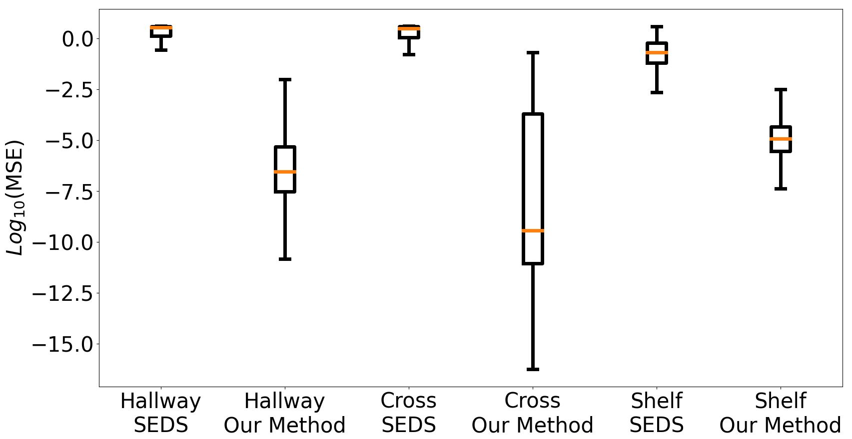
As for the prediction error, we deploy the policy on our validation demonstration dataset and compare the prediction velocities with the demonstrations. The errors for our method and the baseline on the 2D environments are summarized in Fig 8. We can see that our method has a much lower MSE than the baseline. This is due to the policy not being restricted by the quadratic Lyapunov function.

We collected $1209$ demonstrations by sampling a grid of start positions and select valid positions for trajectory optimization. Some example trajectories are shown in Fig. 9(b). The network architecture used to learn the model is found in Appendix. The obstacle avoidance module was added so that the payload does not collide with the shelf.

The results are summarized in Fig. 10. The outcome of the baseline does not match the demonstrations and collide with the shelf (Fig. 10(a)). With collision avoidance, the motion looks closer to the demonstrations, but solely due to the modulation forcing the movement in the same direction of the obstacle (Fig. 10(c)). From Fig. 10(b) and Fig. 10(d), our method reproduces the motion with or without the obstacle avoidance module. In all cases, the policy rollouts reach the goal. From the prediction error in Fig. 8, we see that, again, our method has much lower MSE than the baseline.

Fig. 11 is a visualization of our learnt Lyapunov function. The x-axis is the time-step $n$, and the y-axis is the Lyapunov function output $\tilde{V}\left({\mathbf{x}[n]}\right)$ normalized by the output at initial positions $\tilde{V}\left({\mathbf{x}[0]}\right)$. Fig. 11(a) and Fig. 11(b) are the outputs of $\tilde{V}\left({\mathbf{x}[n]}\right)$ with the demonstration data and with the policy rollout, respectively. We can see that the Lyapunov function outputs are positive and monotonically decreasing until they reach $0$ at the goal. This shows that our method found a suitable Lyapunov function that explains the data.

We also look at the effect of perturbations on the policy. We find that the policy can robustly recover from external perturbations on the robot, since the policy learns a state dependant motion field from the demonstrations and is guaranteed to reach the goal (see the supplementary video https://youtu.be/_NzE6LxoSx4).

We start the robot from several initial positions and deploy the policy to bring the system to the goal. The policy is used as the motion planner and provides the physical robot the sequence of task-space via points toward the goal. Then, this is controlled through the standard inverse kinematics control. Fig. 1 is an example of the outcome; where Fig. 1(a) shows an example of initial position, Fig. 1(b) is the policy rollout (red), and Fig. 1(c) shows that the robot reaches the target position.

The performance of the policy on the real-world robot can be viewed in the supplementary video. We see that the robot is able to perform the task without making contact with the shelf. In all cases, the policy performs the same in task-space on the real-world system as it did in simulation.

Our method can achieve sim-to-real transfer reliably. This is due to our policy being kinematically planned, (i.e., mapping the positions to the velocities), which is less prone to modelling error. Also, when the Lyapunov stability conditions are enforced, the movement are restricted to the directions of demonstrations and less likely to diverge.

References

- [1] J. T. Betts, “Survey of numerical methods for trajectory optimization,” Journal of guidance, control, and dynamics, vol. 21, no. 2, pp. 193–207, 1998.
- [2] M. Kalakrishnan, S. Chitta, E. Theodorou, P. Pastor, and S. Schaal, “Stomp: Stochastic trajectory optimization for motion planning,” in IEEE international conference on robotics and automation, 2011, pp. 4569–4574.
- [3] J. Schulman, J. Ho, A. X. Lee, I. Awwal, H. Bradlow, and P. Abbeel, “Finding locally optimal, collision-free trajectories with sequential convex optimization.” in Robotics: science and systems, vol. 9, no. 1. Citeseer, 2013, pp. 1–10.
- [4] J. Schulman, Y. Duan, J. Ho, A. Lee, I. Awwal, H. Bradlow, J. Pan, S. Patil, K. Goldberg, and P. Abbeel, “Motion planning with sequential convex optimization and convex collision checking,” The International Journal of Robotics Research, vol. 33, no. 9, pp. 1251–1270, 2014.
- [5] M. Bojarski, D. Del Testa, D. Dworakowski, B. Firner, B. Flepp, P. Goyal, L. D. Jackel, M. Monfort, U. Muller, J. Zhang, et al., “End to end learning for self-driving cars,” arXiv preprint arXiv:1604.07316, 2016.
- [6] H.-C. Lin, M. Howard, and S. Vijayakumar, “A novel approach for representing and generalising periodic gaits,” Robotica, vol. 32, no. 8, pp. 1225–1244, 2014.
- [7] P. Abbeel and A. Y. Ng, “Apprenticeship learning via inverse reinforcement learning,” in Proceedings of the twenty-first international conference on Machine learning, 2004, pp. 1–8.
- [8] J. Ho and S. Ermon, “Generative adversarial imitation learning,” Advances in neural information processing systems, vol. 29, 2016.
- [9] I. Goodfellow, J. Pouget-Abadie, M. Mirza, B. Xu, D. Warde-Farley, S. Ozair, A. Courville, and Y. Bengio, “Generative adversarial nets,” in Advances in neural information processing systems, vol. 27, 2014.
- [10] S. M. Khansari-Zadeh and A. Billard, “Learning stable nonlinear dynamical systems with gaussian mixture models,” IEEE Transactions on Robotics, vol. 27, no. 5, pp. 943–957, 2011.
- [11] N. Figueroa and A. Billard, “Locally active globally stable dynamical systems: Theory, learning, and experiments,” The International Journal of Robotics Research, 2022.
- [12] H. Dai, B. Landry, L. Yang, M. Pavone, and R. Tedrake, “Lyapunov-stable neural-network control,” Robotics: Science and Systems, 2021.
- [13] F. Berkenkamp, M. Turchetta, A. Schoellig, and A. Krause, “Safe model-based reinforcement learning with stability guarantees,” in Advances in neural information processing systems, vol. 30, 2017.
- [14] C. W. Warren, “Global path planning using artificial potential fields,” in IEEE International Conference on Robotics and Automation, 1989, pp. 316–317.
- [15] S. M. Khansari-Zadeh and A. Billard, “A dynamical system approach to realtime obstacle avoidance,” Autonomous Robots, vol. 32, no. 4, pp. 433–454, 2012.
- [16] L. Huber, A. Billard, and J.-J. Slotine, “Avoidance of convex and concave obstacles with convergence ensured through contraction,” IEEE Robotics and Automation Letters, vol. 4, no. 2, pp. 1462–1469, 2019.
- [17] L. Huber, J.-J. Slotine, and A. Billard, “Avoiding dense and dynamic obstacles in enclosed spaces: Application to moving in crowds,” IEEE Transactions on Robotics, 2022.
- [18] N. P. Bhatia and G. P. Szegö, Stability theory of dynamical systems. Springer Science and Business Media, 2002.
- [19] E. G. Gilbert, D. W. Johnson, and S. S. Keerthi, “A fast procedure for computing the distance between complex objects in three-dimensional space,” IEEE Journal on Robotics and Automation, vol. 4, no. 2, pp. 193–203, 1988.
- [20] G. Van Den Bergen, Collision detection in interactive 3D environments. CRC Press, 2003.
- [21] C. J. Ong and E. G. Gilbert, “The Gilbert-Johnson-Keerthi distance algorithm: a fast version for incremental motions,” vol. 2, pp. 1183–1189, 1997.
- [22] A. Coulombe and H.-C. Lin, “High precision real time collision detection,” arXiv preprint arXiv:2007.12045, 2020.
- [23] A. Wächter and L. T. Biegler, “On the implementation of an interior-point filter line-search algorithm for large-scale nonlinear programming,” Mathematical programming, vol. 106, no. 1, pp. 25–57, 2006.
- [24] A. Paszke, S. Gross, F. Massa, A. Lerer, J. Bradbury, G. Chanan, T. Killeen, Z. Lin, N. Gimelshein, L. Antiga, A. Desmaison, A. Kopf, E. Yang, Z. DeVito, M. Raison, A. Tejani, S. Chilamkurthy, B. Steiner, L. Fang, J. Bai, and S. Chintala, “Pytorch: An imperative style, high-performance deep learning library,” vol. 32, pp. 8024–8035, 2019.
- [25] E. Coumans and Y. Bai, “Pybullet, a python module for physics simulation for games, robotics and machine learning,” http://pybullet.org, 2016–2021.