Benchmarking Graph Neural Networks
for FMRI analysis
Abstract
Graph Neural Networks (GNNs) have emerged as a powerful tool to learn from graph-structured data. A paramount example of such data is the brain, which operates as a network, from the micro-scale of neurons, to the macro-scale of regions. This organization deemed GNNs a natural tool of choice to model brain activity, and have consequently attracted a lot of attention in the neuroimaging community. Yet, the advantage of adopting these models over conventional methods has not yet been assessed in a systematic way to gauge if GNNs are capable of leveraging the underlying structure of the data to improve learning. In this work, we study and evaluate the performance of five popular GNN architectures in diagnosing major depression disorder and autism spectrum disorder in two multi-site clinical datasets, and sex classification on the UKBioBank, from functional brain scans under a general uniform framework. Our results show that GNNs fail to outperform kernel-based and structure-agnostic deep learning models, in which 1D CNNs outperform the other methods in all scenarios. We highlight that creating optimal graph structures for functional brain data is a major bottleneck hindering the performance of GNNs, where existing works use arbitrary measures to define the edges resulting in noisy graphs. We therefore propose to integrate graph diffusion into existing architectures and show that it can alleviate this problem and improve their performance. Our results call for increased moderation and rigorous validation when evaluating graph methods and advocate for more data-centeric approaches in developing GNNs for functional neuroimaging applications.11 1 Our code is publicly available at https://github.com/elgazzarr/fMRI-GNNs
Keywords graph neural networks functional connectivity major depression disorder autism spectrum disorder functional magnetic resonance imaging
1 Introduction
Mapping the underlying functional brain activity to observed phenotypes and neurological disorders has been a major goal of neuroimaging research. The emergence of non-invasive imaging techniques such as functional magnetic resonance imaging (fMRI) that estimates the neural activity of the brain by measuring the blood-oxygen level dependence (BOLD) has been paramount in advancing our understanding of the functional organization of the brain(Huettel et al. 2004). Yet, modeling the fMRI signal is a challenging feat due to the high dimensionality of the signal coupled with the low sample size, especially in clinical datasets, and the low signal-to-noise ratio of the scans. To build learning models from such data, researchers must opt for tools that incorporate priors from the data structure to guide modeling. This is also called finding the correct inductive bias. Given our knowledge that the brain functions a network Sporns et al. 2005, graph-based methods have been instrumental in modeling the brain with the field of network neuroscience utilizing graph theory approaches to find interesting insights about the brain function and dysfunction (Sporns 2018). With the rise of deep learning, GNNs have been developed to extend the merits of neural networks to graph structured data (Bronstein et al. 2017). Naturally, the neuroimaging community has picked up GNNs and applied it to wide range of tasks such as phenotype prediction (Ktena et al. (2017; Parisot et al. (2018), disease diagnosis (Gallo et al. (2021; Li et al. 2020) and task inference (Li et al. 2019). This adoption is still in its infancy, where most of the work is focused on adapting a specific architecture proposed on other domains for a specific neuroimaging application. It therefore remains unclear which graph architecture should be selected. Should we use graph convolution (Kipf and Welling 2016) as (Gallo et al. (2021) or Graph isomorphic networks (Xu et al. 2018) as in (Kim and Ye 2020). Should we use graph attention (Velic´ et al. 2017) as in (Hu et al. 2021). Should the input graph be static or dynamic (El-Gazzar et al. 2021)? How to create the edges? What is the sample size suitable for training these models? And most importantly, are these techniques capable of exploiting the underlying structure of the data to improve learning?
Despite the theoretical appeal of the application of GNNs to learn from functional brain activity, we find that similar to others domains, the experimental settings for GNNs in neuroimaging applications are in many cases ambiguous or not reproducible (Errica et al. 2019). Some of the most common reproducibility problems concern hyperparameters selection, where hyperparameters optimization is conducted for the proposed model and not the baselines, or they are optimized based on their performance on the final test set. Another main issue is the incorrect use of data splits for model selection versus model assessment. These limitations could lead to over-optimistic and biased estimates of the true performance of the model, making it difficult to assess the advantage of adopting GNNs for this application or to identify the key components in developing more powerful architectures.
With this premise, our primary aim is to provide the neuroimaging community with a fair performance comparison among some of the popular GNN approaches recently adopted for classification of phenotypes or psychiatric disorders from resting-state fMRI scans. We conducted a large number of experiments within a standardized and rigorous model selection and assessment framework for three different large-scale dataset encompassing three different classification tasks. Namely, the Rest-meta-mdd (Yan et al. 2019) dataset for the classification of major depression disorder, the Autism Brain Imaging Data Exchange (ABIDE I+II) (Martino et al. 2014) dataset for the classification of autism spectrum disorder and the UkbioBank (Sudlow et al. 2015) dataset for sex classification.
Secondly, we aim to identify if and to what extent current approaches can effectively exploit graph structures. To this end, we implement three structure-agnostic baselines, whose purpose is to disentangle the advantage of graph structure information from the nodes features. To ensure a fair comparison against GNN methods, we conduct our baseline experiments under a similar framework for hyperparameter optimization and model selection and assessment.
Our third aim is to study the effect of scaling the sample size on the GNNs and the baselines. We evaluate the performance of the models when trained on different sample sizes on the UkbioBank for sex classification and tested on an independent subset.
Finally and most importantly moving forward, our objective is to apply insights from our implementations and empirical results to highlight strengths and shortcomings of current methods and propose a set of recommendations to help utilize the potential of this powerful set of tools.
2 Background
Graph neural networks are a class of neural networks that extend deep learning to graph structured data, and have been utilized in several domains for tasks such as node classification, edge prediction and graph classification (Bronstein et al. 2017; Zhou et al. 2020; Wu et al. 2019). While graph neural networks have been applied for node classification tasks in functional neuroimaging where the graph represented a population graph (Parisot et al. (2018), a more befitting application is graph classification, where a brain is represented as a mathematical graph whose nodes represent brain regions and edges constitute their connections. Input graphs for GNN models are often attributed graphs with the attributes representing the node features . A graph can be stationary or dynamic depending on the evolution of the features and/or connections across time. This work addresses the task of graph classification from both static and dynamic functional graphs and using five popular GNN architectures. Our criteria for selection are i) popularity i.e. the architecture has been extensively validated in multiple domains for applications and is commonly used as a benchmark in graph neural networks surveys; ii) strong architectural differences; iii) original code publicly available; iv) previous adaptation on fMRI data. Specifically, we adopt Graph Convolutional Networks (GCNs), Graph Attention Networks (GATs), Graph Isomorphic Networks (GINs) as architectures to learn from static graphs. While for dynamic graphs, we adopt Spatio-Temporal Graph Convolutional Networks (ST-GCNs) and Adaptive Spatio-Temporal Graph Convolutional Networks (AST-GCNs). Several architectural choices for each model are represented as parameters in a search space and are selected using an exhaustive hyperparameter search. Thus each of the models can be viewed as a general class that encompasses several variants of previously proposed GNN models. We briefly describe the main idea behind each class and some of their previous applications for learning from fMRI data. We discuss the specific details of each method under a uniform framework in Section 3.2.
Graph convolutional networks
A GCN (Kipf and Welling 2016) can be viewed as the counterpart of a convolutional neural network (CNN) model for graph-structured data that uses a graph spectral approach to perform convolution. A graph convolutional layer extracts features through a first-order spectral approximation of the graph by restricting the filters (limiting the order of the Chebyshev polynomial) to operate in the neighborhood at one step away from each node. GCNs are the most popular method applied for graph classification from fMRI data and have been utilized for the diagnosis of psychiatric disorders such as ASD (Arya et al. 2020; Li et al. 2020; Ktena et al. (2017), MDD (Gallo et al. (2021; Qin et al. 2022) and Schizophrenia (Oh et al. 2022; Lei et al. 2022).
Graph attention networks
GAT (Velic´ et al. 2017) is a graph neural network architecture that uses the attention mechanism to learn weights between connected nodes. In contrast to GCN, which uses predetermined weights for the neighbors of a node corresponding to the normalization coefficients, GAT modifies the aggregation process of GCN by learning the strength of the connection between neighboring nodes through the attention mechanism on the features of the connected nodes. (Li et al. 2019; Li et al. 2020) have adopted GATs for the diagnosis of ASD.
Graph isomorphic network
GINs were proposed by (Xu et al. 2018) as a special case of spatial GNN suitable for graph classification tasks. The network uses the sum operation to aggregate features from the neighboring nodes and employs an extra fully connected layer in a non-linear multi-layer perceptron (MLP) to transform the output at each layer. The authors argue the GINs can learn an invective function which deems the model to be possibly as powerful as the Weisfeiler-Lehman test (Weisfeiler and Leman 1968) for graph classification tasks. (Kim and Ye 2020)) have applied GINs for sex classification from rs-fMRI data.
Spatio-temporal graph convolution network
ST-GCNs (Yu et al. 2017) has been first proposed to model dynamic data for the application of traffic forecasting. They were developed to extract features from graphs with dynamic attributes that evolve with time and have been popular in several applications such as weather forecasting and skeleton-based activity recognition. A typical ST-GCN block consists of a temporal layer (e.g. 1D Conv layer, LSTM, etc.) to extract temporal features followed by a graph convolution layer for spatial feature extraction. Stacking ST-GCN blocks enables spatio-temporal feature extraction.(Gadgil et al. 2020) and (Azevedo et al. 2020) have applied ST-GCNs on fMRI data the tasks of sex and age classification, and (Kong et al. 2021) for the task of MDD diagnosis.
Adaptive spatio-temporal graph convolution network
AST-CGNs (Bai et al. 2020) fundamentally share the same concept as ST-GCNs in feature extraction however they differ in the input graph structure. While ST-GCN relies on a predefined adjacency matrix, AST-GCN starts with a randomly initialized graph structure and adaptively learns the optimal graph structure through gradient descent in an end-to-end fashion. While computationally more expensive, this setup enables learning task-specific graph structure in domains where there is no known graph structure or the predefined graph structure is not sufficient. (El-Gazzar et al. 2021) have applied AST-GCN for the tasks of sex and age classification.
3 Methods
3.1 Graph creation
This work studies both static and dynamic representation of graphs. Static graphs assume no temporal evolution of the graph structure and nodes features. They are typically created solely using static measures of similarity (e.g. correlations) for both the edges and features. Currently, the most popular approach for static graph creation is using the Pearson correlation of the ROIs time-courses (commonly refereed to as functional connectivity) to define the nodes features as the connectivity profile of each ROI (the respective row of the correlation matrix) and the graph edges are represented as a sparse version of the correlation matrix. Note that while some works use other approaches such as clustering, structural connectivity and anatomical location for representing graph edges, the use of functional connectivity (FC) to define graph structure remains the most popular approach in the large majority of GNN brain studies. In this work we follow the same popular strategy to create static graphs and use GCN, GAT, and GIN models for learning from static graphs while treating the sparsfication threshold as a tunable hyperparamter. The threshold is set based on a proportional thresholding (i.e. selecting strongest PT % connections) rather than absolute threshold as it has shown in graph to have improved test-retest reliability and is less sensitive to variation in graph density (Braun et al. 2012; Van Wijk et al. 2010). Static graphs are relatively easier to compute, have more training architectures to select from, have a significantly lower number of dimensions and a more robust to physiological noise and inter-scanner variability. However, they fail to represent the dynamic nature of brain activity which is hypothesized to contain the biomarkers for mental disorders (Hutchison et al. (2013).
Dynamic graphs enable modelling such dynamic signal by representing the nodes features as ROIs time-courses. Similar to static graphs, dynamic GNNs employ thresholded FC to define the graph adjacency matrices. Another strategy adopted by (El-Gazzar et al. 2021), is to randomly initialize the adjacency matrix and adaptively learn its weights in an end-to-end manner simultaneous with the GNN weights via gradient descent. We adopt the former strategy for our ST-GCN model and the latter for the AST-GCN model. Figure 1 summarizes the graph creation strategy employed for all 5 models in this study.

3.2 Graph Neural Networks
For graph classification, the goal of a GNN is to learn a function which maps a graph to a feature vector that summarizes the graph and contains information necessary for classification. The forward function thus can be viewed as :
| (1) |
where is the label of the graph and is a function parameterized by a neural network to map the output feature vector of the GNN to the label. In this work, we choose as a single-layer fully connected neural network for all the different GNN architectures. Thus, the empirical results would only reflect how powerful are different parameterizations of in representing the graph signal and structure. In this section, we explain how each GNN architecture models this function.
3.2.1 GCNs
A GCN learns graph representations via an approximation of spectral convolutions on the graphs. Spectral convolutions on graphs is defined as the multiplication of the the graph signal with a filter in the Fourier domain.
| (2) |
where is the matrix of eigenvectors of the normalized graph Laplacian with a diagonal matrix of its eigenvalues and being the graph Fourier transform of . Evaluating this spectral convolution in its current form is computationally expensive because of the multiplication by and the eigendecomposition of . (Hammond et al. 2011) suggested that can be well-approximated by a truncated expansion in terms of Chebyshev polynomials up to K-th order. Follow up work by (Kipf and Welling 2016) proposed to restrict the polynomials to their first order for each graph convolutional layer and stacking graph convolutional layer to recover a rich class of convolutional filters. The layer-wise propagation rule of the GCN can thus be defined in the spatial domain as :
| (3) |
where is the graph signal representation at layer ; , is the adjacency matrix with self-connections, is the degree matrix, is a trainable weight matrix and denotes a non-linear activation function. (Gilmer et al. 2017) later formalized this definition as message passing and update operations on the nodes. The node-wise update rule for a GCN can thus be defined as
| (4) |
where and are the message and update functions respectively, is the edge weight between nodes and (set to 1 in unweighted graphs) and is the neighborhood of the node . In this work, we set as we observed no additional gain from convolving higher-order neighborhoods of the graph nodes. is a linear fully connected layer and is a is a single-layer feed forward network with a hidden dimension set as a hyperparameter with a non-linear ReLU(·) activation function.
3.2.2 GATs
The main difference between a GCN and GAT layer lies in the permutation invariant update function applied to each node i to combine the node features hi with its aggregated neighborhood features (transformed by some function ) and update its representation. In GCNs, importance of node j to node i’s representation is defined using , the entry on the normalized adjacency matrix. For GATs, the importance is learned implicitly using a self-attention mechanism. Formally, the update rule for each node in a GAT layer can be defined as:
| (5) | |||
| (6) |
denotes a concatenation operation, is a non-linear activation function and is a trainable single-layer feed-forward neural network. This attention mechanism can be extended to a multi-head attention via learning M different copies of and calculating their average. In this work, we treat as a hyperparameter with an option of setting given that the sample size is limited and increasing the model trainable parameters by a large factor can lead to over-fitting. We follow the author’s recommendation of choosing as LeakyReLU( ) and parameterizing the linear transformation of the feature vectors via a linear layer. For the rest of the parameters of the GAT model (Number of layers, size of the hidden dimension and graph readout layer), we follow the same setting as described in Section 4.1.1
3.2.3 GINs
The Graph Isomorphism Network (GIN) is a variant of the GNN suitable for graph classification tasks, which is known to be as powerful as the WL-test under certain assumptions of injectivity. Unlike GCNs and GATs which can use any permutation invariant function to aggregate neighborhood features, GINs typically only use the sum operation and do not include a transformation function before combining the neighborhood features with the original node features. Rather, a multi-layer perceptron (MLP) is applied directly on the combined features. The update rule for each node in a GIN layer be defined as:
| (7) |
where is a learnable parameter initialized to zero. The purpose of this parameter is to learn the amount of original information in the node that it should retain in the next representation. We use a two layer with ReLU() as non-linearity and as recommended by the paper. For the READOUT layer, we experiment with the three permutation invariant functions as in Section 4.1.1.
3.2.4 ST-GCNs
ST-GCNs model graphs with dynamic features by utilizing spatio-temporal blocks that alternate between sequence-to-sequence layers for learning temporal features, and graph convolutions for spatial feature extraction. While there has been several variants of ST-GCNs that differ either in the number or order of layers in the ST-GCN block, or the the temporal learning layer (e.g., gated temporal convolutions, dilated convolutions, LSTMs), we follow the work by (Wu et al. 2019) to implement our variant of ST-GCN for fMRI as we have observed it provided the most stable results across tasks. Namely, we utilize a cascade of St-GCN blocks for spatio-temporal feature extraction, where each ST-GCN block consists of a one layer of gated temporal convolution (GATED-TCN) for temporal feature extraction followed by a spatial graph convolution as described in Section for spatial feature extraction. For a node input representation where is the number of channels, a Gated-TCN extracts temporal feature representation as follows:
| (8) |
where and are the weights of two parallel 1D convolutions for controlling the flow of information into the next layer, and are the biases and represent the Hardmard product operation. The extracted feature representations are then treated as the nodes input representation in a GCN and is processed similar to Equation 4. Another key difference between the ST-GCN employed this work and prior implementations of ST-GCNs for modelling fMRI data is that we use the entire timecourses for the duration of the scan as the node features as opposed to previous works by (Gadgil et al. 2020) (Azevedo et al. 2020) who use crops of . We found that cropping the timecourses for training and aggregating the predictions during inference drastically deteriorates the performance for the clinical tasks.
3.2.5 AST-GCNs
In multiple spatio-temporal datasets, we know that the underlying interaction between the temporal features can be modelled as a graph, but we don’t have access to the ground truth structure of the graph. Adaptive learning of graph structure is a growing area of research in the field of GNNs and several variants have been proposed by the research community in recent years (Bai et al. 2020), (Wu et al. 2019), (Wu et al. 2020). AST-GCNs can be generalized as ST-GCNs equipped with a graph structure learning module. In this work, we follow the implementation of (Bai et al. 2020) which defines the normalized adjacency matrix as
| (9) |
where is a learnable node embedding dictionary initialized randomly with dimension as a hyperparameter. Multiplying the dictionary by its transpose results in a dense symmetric matrix, which is then passed through a activation function to eliminate weak connections and then row-normalized using the Softmax operation. We also experimented with the Sparsemax operation (Martins and Astudillo 2016) and found that it improved stability during learning. The rest of our AST-GCN implementation is kept similar to our ST-GCN to disentangle the effect of adaptive learning of the graph structure.
3.3 Graph Readout
Following feature extraction using any of the proposed GNN architectures, the readout phase computes a feature vector for the whole graph using some permutation-invariant readout function to be passed as an input to the final classification layer. In this work we experiment with 3 different permutation-invariant functions to summarize the graph features after the last graph layer. Namely Mean(), Mean()Max() and Sum(). The selection of which function to use for each architecture/dataset combination is set as a hyperparameter. We empirically observe that Mean() and Mean()Max() provide the most stable results to all GNN architectures with exception of the GIN architecture where the Sum() operation marginally improve the performance of the model.
4 Data & Experimental Setup
4.1 Datasets
Throughout this study we evaluate the performance of the models on three different datasets, each with a different classification target and a different prepossessing pipeline. This setup enables us to make a generalized conclusion from the empirical results that are robust to variation in demographics, classification target, pre-processing pipeline and data acquisition protocols.
ABIDE I+II contains a collection of rs-fMRI brain images aggregated across 29 institutions. It includes data from participants with a clinical diagnosis of autism spectrum disorder and typically developing participants (TD). In this study, we select a subset of the dataset with N = 1207 (558 TD/649 ASD) using the largest nine sites in terms of number of participants (N50) to conduct our analysis. The 4D volumes were pre-processed according to the CPAC pipeline (Craddock et al. (2013b) with the same parameters as in (Craddock et al. (2013a). Further, the craddock-200 (Craddock et al. 2012) atlas was used to parcellate the volume into 200 regions of interest (ROIs) and the timecourses of each region were calculated as the mean signal between all the voxels of the ROI.
Rest-meta-MDD is currently the largest open-source rs-fMRI database for studying major depression disorder including clinically diagnosed patients and healthy controls from 25 cohorts in China. In this study we select a subset of the dataset with N = 1453( 628 HC/825 MDD) using the largest 9 sites (N 40). Standard pre-processing of the data was done at each site using the Data Processing Assistant for Resting-State fMRI (DPARSF) (Yan and Zang 2010) and 112 timecourses of cortical and sub-cortical regions as defined by the Harvard-Oxford atlas (Makris et al. (2006) were extracted.
UkBioBank is a large-scale biomedical database and research resource, containing in-depth genetic and health information from half a million UK participants. In this work we use a subset with (N=5500 (2750 M/ 2750 F)) randomly sampled from the first release. The dataset provides the pre-processed 4D volumes in MNI format. These volumes were then parcellated to 116 anatomical regions using the automated anatomical labeling (AAL) atlas (Tzourio-Mazoyer et al. (2002) and the mean timecourse of each region was extracted.
4.2 Model selection & assessment
For a fair evaluation of the methods, we constructed a systematic pipeline to find the optimal performance of each of the methods. This constitutes using a configuration of hyperparameters for each model that are optimal for the given task. A common pitfall in hyperparameter tuning is conducting the search based on the performance of the final test set. This results in an over-optimistic estimate of the model generalization capability. In this work, we conducted hyperparameter search for each GNN model on a held out validation set for each dataset. We conducted an exhaustive hyperparameter search on the key parameters that could influence the convergence of the model and its performance. While some of the parameters are exclusive to some architectures (e.g. the number of attention heads in the GAT), the majority of hyperparameters and their search spaces were shared across methods (See Table S1 for details on the hyperparameters and their search spaces). This enables a relatively fair evaluation of each architecture. After finding the best hyperparameter configuration for each model and the respective tasks, we followed a 5-fold cross validation scheme with model selection using the lowest loss value on an inner validation split (85/15 training/validation split) for the Rest-meta-MDD and ABIDE I+II datasets. For the UkBioBank dataset, the models are trained on subsets of the full sample (N = [500, 1000, 2000, 5000]) with a similar inner validation split for model selection and the test results are reported on a fixed independent set of N = 500 to evaluate the effect of training sample size on the performance. (See Supplementary information for details about training procedure)
4.3 Non-graph baselines
To fairly judge whether GNNs are fully capable of leveraging the graph structure, their performance need to be evaluated against baselines that are not inductively aware of the structure of the data, and a similar framework should be followed for hyperparameter search and model selection. In this work we employ three different structure-agnostic baselines. Specifically, we adopt a multi layer perceptron (MLP), support vector machines with radial basis function kernel (SVM-rbf) as baselines for learning from static representations. The input to these models are the flattened lower-triangular matrix of the correlation matrix. For a baseline that learns from dynamic representations, we used 1D CNNs similar to (El Gazzar et al. 2019). The inputs to the 1D CNN are the prepossessed ROI time-courses stacked as channels. (See Supplementary information for details about training the baselines and their hyperparameters)
| Rest-meta-MDD | ABIDE I+II | ||||||
|---|---|---|---|---|---|---|---|
| Models | Acc. % | Sens. % | Spec. % | Acc. % | Sens. % | Spec. % | |
| GCN | 62.6 ± 3 | 57.6 ± 8 | 67.8 ± 8 | 67.6 ± 2 | 69.5 ± 4 | 65.7 ± 3 | |
| GIN | 62.7 ± 3 | 67.3 ± 5 | 58.1 ± 3 | 68.5 ± 1 | 81.7 ± 3 | 55.4 ± 4 | |
| Static GNNs | GAT | 62.9 ± 2 | 69.5 ± 3 | 56.4 ± 5 | 68.2 ± 2 | 63.5 ± 5 | 72.9 ± 3 |
| ST-GCN | 58.2 ± 4 | 48.6 ± 8 | 67.8 ± 9 | 65.3 ± 2 | 67.2 ± 4 | 63.4 ± 4 | |
| Dynamic GNNs | AST-GCN | 60.7 ± 2 | 44.6 ± 2 | 75.8 ± 8 | 67.8 ± 2 | 70.8 ± 5 | 64.9 ± 3 |
| 1D CNN | 63.2 ± 3 | 68.5 ± 5 | 59.6 ± 6 | 70.6 ± 2 | 72.7 ± 3 | 68.5 ± 3 | |
| SVM-rbf | 61.9 ± 2 | 79.0 ± 5 | 44.9 ± 5 | 69.5 ± 2 | 75.9 ± 3 | 63.0 ± 3 | |
| Baselines | MLP | 58.4 ± 4 | 60.1 ± 2 | 56.8 ± 3 | 66.6 ± 2 | 72.1 ± 1 | 61.2 ± 2 |
5 Results
5.1 Disorder diagnosis
The results in Table 1 show the test performance of the GNNs and baselines on the clinical datasets. On the clinical tasks (N=1207 and N=1453), all the GNNs perform competitively where no one architecture significantly superior to the others. A notable observation is that static GNNs marginally outperformed dynamic GNNs. This contradicts the main hypothesis that dynamic representations are more faithful to natural dynamics of brain activity over summarized static correlation values and thus would result in better results. This is however true for the dynamic baseline, where the 1D CNN outperformed all the methods on both tasks. In general, graph-agnostic baselines performed on par with or marginally outperformed GNN methods despite having no awareness of the structural organization of the data. These empirical results raise even more questions; do GNNs simply fail to leverage the graph structure in learning better representations and hence obtain superior results, or do the heterogeneity of the data and possible noise in the clinical labels create an upper bound on the performance of the models, rendering quantitative evaluation of the merits of GNNs challenging? How does the sample size affect the performance of these models?
5.2 Scaling performance on the UKBioBank
To shed light on some of these questions, we can look at the scaling performance of these models on the UkBioBank at different training samples on the task of sex classification. Figure 2 shows that, similar to the clinical datasets, 1D CNN outperform the rest of the methods at all samples instances. This is especially clear on the smaller sample sizes (N=500 and N=1000). This gap is then reduced at the larger sample sizes, where the dynamic AST-GCN model show improved scaling performance and eventually catch up to the 1DCNN. Again, while these results emphasize the benefits of incorporating the dynamic signal, it questions the sample-efficiency of GNN models in clinical applications, especially since the motivation behind adopting GNNs is that incorporating inductive bias about the structure of the data should alleviate the need for larger sample sizes to learn this solely from data. An advantage we unfortunately do not observe in our empirical results.
A key property of AST-GCN is that it does not require specifying the graph structure in advance, and is jointly learned using gradient descent along with the rest of the model at the cost of extra training parameters. The scaling behaviour of AST-GCN is thus empirically justified and similar scaling performance was previously reported for adaptive spatio-temporal GNNs (El-Gazzar et al. 2021; Wu et al. 2020). The performance of AST-GCN however, attest against the correctness of the graph structure of the data used as input to the rest of the GNN models. As we highlighted in Section 3.1, unlike several graph-structured data, there is no ground truth network structure for the brain and thus defining adjacency matrix of fMRI graphs is rather an arbitrary process with most works opting for FC for this role. In this work, we followed a similar strategy in effort to evaluate the performance of GNN models. The results of our experiments invites us to rethink about this aspect and to find more principled approaches to accommodate this problem. The results of AST-GCN guide toward end-to-end learning of the graph structure as a potential solution to this problem. This however, comes at the expense of large training samples, a luxury not available in most of clinical datasets.
5.3 Graph diffusion improves learning on noisy graphs
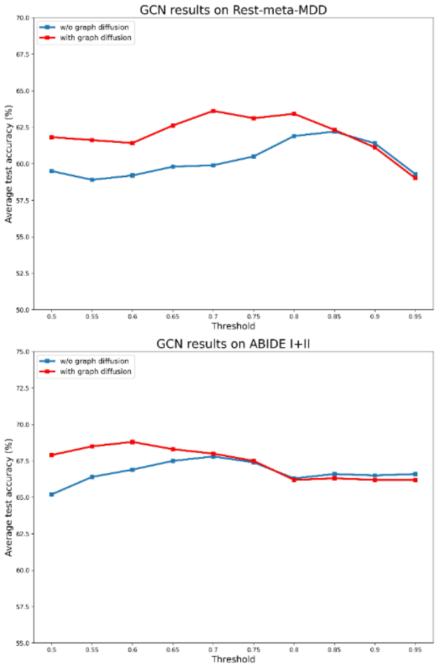
In network neuroscience, data-driven analysis on thresholded connectivity graphs are acknowledged to be potentially problematic, where different thresholding techniques and values and can lead to the inclusion of spurious connections confounding the analysis (van den Heuvel et al. 2017; Van Wijk et al. 2010; Fornito et al. 2012). Yet we argue that this remains an overlooked problem when using GNNs. During the course of this work, we treated the sparsfication proportional threshold as a hyperparameter that is selected based on the best performance on a validation set. While conducting the experiments, we observed a high sensitivity of the results to the sampled sparsfication threshold. Further, we observed different optimal thresholds for each task and GNN class. In Figure 3, we present the results of the GCN model on the two clinical datasets with all parameters fixed and using sparsfication thresholds in the range of [50, 95] % with a step size of 5 %. The empirical results show that selecting an optimal threshold plays an important role in the final evaluation performance and attest against arbitrary threshold selection (e.g. 50 % as is the current practice) in creating input graphs for GNNs. Further, improved performance at higher thresholds (70-85%) highlights that proportional thresholding of FC results in noisy graphs. In graph theoretical analysis, proposals to mitigate this problem are to include graph density as a covariate or to adjust the null distribution to account for random edges resulting from thresholding low density graphs (van den Heuvel et al. 2017). An open question is how to deal with such noisy FC graphs while training GNNs on fMRI data.
A possible solution to dealing with noisy graphs is graph diffusion convolution (GDC) (Klicpera et al. 2019). Where instead of aggregating information only from the first-hop neighbors, GDC models message passing between nodes as a generalized continuous diffusion process defined by the diffusion matrix
| (10) |
with the weighting coefficients , and the generalized transition matrix . In principle, one can choose different methods to define the coefficients and the transition matrix provided that Eq. 10 converges. Diffusion coefficients can be defined using well-studied functions such as the heat kernel (Kondor and Lafferty 2002), personalized page rank (PPR) (Brin and Page 1998) or even learned using gradient descent. Popular examples of defining the transition matrix are the random walk transition matrix and the symmetric transition matrix . Essentially by restricting the sum in Eq. 10 to a finite number of steps , and choosing suitable diffusion parameters, GDC transforms the original potentially noisy adjacency matrix into a new graph where any GNN model can be applied. This transformation has been shown to consistently improve the performance of GNN models on several real world graph datasets. In Fig 3, we show the effect of applying graph diffusion using the heat kernel coefficient and the symmetric transition matrix with on the GCN model on the two clinical datasets at different sparsification thresholds compared to using the original defined graph structure without any transformation (i.e. setting , and ). The results show that by simply incorporating this transformation as a prepossessing step, the performance of the model is less sensitive to the sparsfication threshold at lower thresholds and can even improve the empirical results without the need for expensive hyperparameter search for the optimal sparsfication threshold.
6 Discussion
The rapid pace of adoption of GNNs in neuroimaging applications urges us to pause and ponder about the rationale and success of this adoption. While we agree that the motivation is well-grounded in the field and in fact necessary for sample-efficient factual learning models, we question whether the current methods are living up to the promises of the motivation. We argue that it is difficult to answer this question without a systematic evaluation of the methods and their current alternatives under a uniform fair setup. In this study, our aim was to build such a framework by benchmarking popular classes of GNN architectures through the applications of brain disorder diagnosis and phenotype prediction. The choice of the application is motivated by the trend and interest of the researchers to use GNNs for such tasks and the open-source nature of the datasets. In building our framework, we strive for a rigorous fair and setup through i) uniform model selection and assessment strategies across methods, ii) fair allocation of computational resources to all the methods by providing an exhaustive range of parameter search spaces for each architecture/task combination to obtain the best possible performance for each method iii) uniform training setup (e.g. loss functions, regularization, initialization schemes) for all deep learning methods to disentangle only architectural effects on the performance. Our empirical results show that, on average, GNNs fail to outperform current learning alternatives, and that and no one GNN architecture was consistently superior over the others. A simple 2 layer 1D CNN where all the ROIs stacked as channels with no structural awareness of the graph consistently outperformed sophisticated structurally aware GNN methods. The results of AST-GCN – a dynamic model that learns the graph structure at the cost of more training parameters – showed an improved performance at the largest sample size over FC-driven graphs. This opens the question whether graph structures defined using thresholded functional connectivity, as is done throughout this work and as is the current practice in the field, is the most optimal strategy for constructing the graphs. We highlighted that thresholded FC is a major issue when computing graph theory measures in network neuroscience, yet, remains an unacknowledged problem in GNNs research. We proposed to integrate graph diffusion as a prepossessing step and show that it can partially alleviate the problem and consistently improve the results. While not the only solution, this calls for a more data-centeric approach when developing learning models from fMRI graphs over a model-centeric approach where we observed that architectural differences did not play an important role in the final outcome in the studied applications. On a more general note, the empirical results open the debate of the utility of deep learning in neuroimaging applications (He et al. 2020; Schulz et al. 2020). On the clinical datasets, the SVM model performed competitively with the DL models without the need for engineering complex neural network architectures. We argue that the competitiveness of DL methods at this scale is a positive rather than a criticism. On the UkBioBank, the dynamic DL models (1D CNN, AST-GCN) do show improved performance over the SVM and other static baselines. This guides towards developing DL models that utilize minimally pre-processed dynamic signal over static feature engineered summaries such as correlation values. Further, to objectively identify the merits of applying GNNs for single-subject prediction we have to look further than the test metrics and consider the advantage of enabling the application of deep learning methods in this domain. DL is a versatile class of algorithms with applications that extend beyond supervised classification and would potentially be of remarkable value when applied on fMRI data. For example, graph explainability techniques (Ying et al. 2019; Huang et al. 2022) could be utilized to find potential functional connectivity biomarkers for phenotypes and psychiatric disorders. The application of graph self-supervised learning techniques Fedorov et al. 2021; Wang et al. 2022; Peng et al. 2022 and graph normative modelling (Gazzar et al. 2022) on non-clinical datasets would assist in learning representations that could further be transferred to a downstream clinical tasks. Graph augmentation methods Zhao et al. 2021 could boost the statistical power of the clinical datasets and assist in solving the problem of labeled data scarcity and regularize overfitting. These are some of the promising directions that support the utility of GNNs in neuroimaging. That said, the empirical results presented in this work advocate for more moderation and more rigorous validation when reporting GNN results that do not clearly outperform graph-agnostic baselines. Finally, we hope that framework developed throughout this work could serve as a baseline for future novel GNN architectures or applications on fMRI data and assist in identifying key components that could improve existing methods.
Acknowledgments
This work was supported by the Netherlands Organization for Scientific Research (NWO; 628.011.023); Philips Research; ZonMW (Vidi; 016.156.318). The access of the UKbioBank data was granted under the application number 30091.
References
- Huettel et al. [2004] S. A. Huettel, A. W. Song, and G. McCarthy. Functional magnetic resonance imaging. vol., 1, 2004.
- Sporns et al. [2005] O. Sporns, G. Tononi, and R. Kotter. The human connectome: a structural description of the human brain. PLoS Computational Biology, 1, 2005.
- Sporns [2018] O. Sporns. Graph theory methods: applications in brain networks. Dialogues in clinical neuroscience, 20:111, 2018.
- Bronstein et al. [2017] M. M. Bronstein, J. Bruna, Y. LeCun, A. Szlam, and P. Vandergheynst. Geometric deep learning: going beyond euclidean data. IEEE Signal Processing Magazine, 34:18–42, 2017.
- Ktena et al. [(2017] S. I. Ktena, S. Parisot, E. Ferrante, M. Rajchl, M. Lee, B. Glocker, et al. Distance metric learning using graph convolutional networks: Application to functional brain networks. pages 469–477. Conference on Medical Image Computing and Computer-Assisted Intervention, (2017).
- Parisot et al. [(2018] S. Parisot, S. I. Ktena, E. Ferrante, M. Lee, R. Guerrero, B. Glocker, et al. Disease prediction using graph convolutional networks: application to autism spectrum disorder and alzheimer’s disease. Medical image analysis, 48:117–130, (2018).
- Gallo et al. [(2021] S. Gallo, A. ElGazzar, P. Zhutovsky, R. M. Thomas, N. Javaheripour, L. Meng, et al. Thalamic hyperconnectivity as neurophysiological signature of major depressive disorder in two multicenter studies. (2021).
- Li et al. [2020] X. Li, N. C. Dvornek, J. Zhuang, P. Ventola, and J. Duncan. Graph embedding using infomax for asd classification and brain functional difference detection. In Medical Imaging, 1317:11317, 2020.
- Li et al. [2019] X. Li, N. C. Dvornek, Y. Zhou, J. Zhuang, P. Ventola, and J. S. Duncan. Graph neural network for interpreting task-fmri biomarkers. In International Conference on Medical Image Computing and Computer-Assisted Intervention, pages 485–493, 2019.
- Kipf and Welling [2016] T. N. Kipf and M. Welling. Semi-supervised classification with graph convolutional networks.arxiv. preprint, 2016.
- Xu et al. [2018] K. Xu, W. Hu, J. Leskovec, and S. Jegelka. How powerful are graph neural networks? arxiv. preprint, 2018.
- Kim and Ye [2020] Byung-Hoon Kim and Jong Chul Ye. Understanding graph isomorphism network for rs-fmri functional connectivity analysis. Frontiers in neuroscience, page 630, 2020.
- Velic´ et al. [2017] P. Velic´, G. Cucurull, A. Casanova, A. Romero, P. Lio, and Y. Bengio. Graph attention networks. preprint, 2017.
- Hu et al. [2021] J. Hu, L. Cao, T. Li, S. Dong, and P. Li. Gat-li: a graph attention network based learning and interpreting method for functional brain network classification. BMC bioinformatics, 22:1–20, 2021.
- El-Gazzar et al. [2021] A. El-Gazzar, R. M. Thomas, and G. van Wingen. Dynamic adaptive spatio-temporal graph convolution for fmri modeling. In International Workshop on Machine Learning in Clinical Neuroimaging., pages 125–134, 2021.
- Errica et al. [2019] F. Errica, M. Podda, D. Bacciu, and A. Micheli. A fair comparison of graph neural networks for graph classification. arxiv. preprint, 2019.
- Yan et al. [2019] C.-G. Yan, X. Chen, L. Li, F. X. Castellanos, T.-J. Bai, Q.-J. Bo, et al. Reduced default mode network functional connectivity in patients with recurrent major depressive disorder. Proceedings of the National Academy of Sciences, 116:9078–9083, 2019.
- Martino et al. [2014] A. D. Martino, C.-G. Yan, Q. Li, E. Denio, F. X. Castellanos, K. Alaerts, et al. Molecular psychiatry, 19:659–667, 2014.
- Sudlow et al. [2015] C. Sudlow, J. Gallacher, N. Allen, V. Beral, P. Burton, J. Danesh, et al. Uk biobank: an open access resource for identifying the causes of a wide range of complex diseases of middle and old age. PLoS medicine e1001779, 12, 2015.
- Zhou et al. [2020] Jie Zhou, Ganqu Cui, Shengding Hu, Zhengyan Zhang, Cheng Yang, Zhiyuan Liu, Lifeng Wang, Changcheng Li, and Maosong Sun. Graph neural networks: A review of methods and applications. AI Open, 1:57–81, 2020.
- Wu et al. [2019] Zonghan Wu, Shirui Pan, Guodong Long, Jing Jiang, and Chengqi Zhang. Graph wavenet for deep spatial-temporal graph modeling. arXiv preprint arXiv:1906.00121, 2019.
- Arya et al. [2020] Devanshu Arya, Richard Olij, Deepak K Gupta, Ahmed El Gazzar, Guido Wingen, Marcel Worring, and Rajat Mani Thomas. Fusing structural and functional mris using graph convolutional networks for autism classification. In Medical imaging with deep learning, pages 44–61. PMLR, 2020.
- Qin et al. [2022] Kun Qin, Du Lei, Walter HL Pinaya, Nanfang Pan, Wenbin Li, Ziyu Zhu, John A Sweeney, Andrea Mechelli, and Qiyong Gong. Using graph convolutional network to characterize individuals with major depressive disorder across multiple imaging sites. EBioMedicine, 78:103977, 2022.
- Oh et al. [2022] Kang-Han Oh, Il-Seok Oh, Uyanga Tsogt, Jie Shen, Woo-Sung Kim, Congcong Liu, Nam-In Kang, Keon-Hak Lee, Jing Sui, Sung-Wan Kim, et al. Diagnosis of schizophrenia with functional connectome data: a graph-based convolutional neural network approach. BMC neuroscience, 23(1):1–11, 2022.
- Lei et al. [2022] Du Lei, Kun Qin, Walter HL Pinaya, Jonathan Young, Therese van Amelsvoort, Machteld Marcelis, Gary Donohoe, David O Mothersill, Aiden Corvin, Sandra Vieira, et al. Graph convolutional networks reveal network-level functional dysconnectivity in schizophrenia. Schizophrenia Bulletin, 2022.
- Weisfeiler and Leman [1968] B. Weisfeiler and A. Leman. The reduction of a graph to canonical form and the algebra which appears therein. NTI, Series, 2:12–16, 1968.
- Yu et al. [2017] B. Yu, H. Yin, and Z. Zhu. Spatio-temporal graph convolutional networks: A deep learning framework for traffic forecasting. arxiv. preprint, 2017.
- Gadgil et al. [2020] S. Gadgil, Q. Zhao, A. Pfefferbaum, E. V. Sullivan, E. Adeli, and K. M. Pohl. Spatio-temporal graph convolution for resting-state fmri analysis. In International Conference on Medical Image Computing and Computer-Assisted Intervention, pages 528–538, 2020.
- Azevedo et al. [2020] T. Azevedo, L. Passamonti, P. Lio, and N. Toschi. Towards a predictive spatio-temporal representation of brain data. arxiv. preprint, 2020.
- Kong et al. [2021] Youyong Kong, Shuwen Gao, Yingying Yue, Zhenhua Hou, Huazhong Shu, Chunming Xie, Zhijun Zhang, and Yonggui Yuan. Spatio-temporal graph convolutional network for diagnosis and treatment response prediction of major depressive disorder from functional connectivity. Human brain mapping, 42(12):3922–3933, 2021.
- Bai et al. [2020] L. Bai, L. Yao, C. Li, X. Wang, and C. Wang. Adaptive graph convolutional recurrent network for traffic forecasting. arxiv. preprint, 2020.
- Braun et al. [2012] Urs Braun, Michael M Plichta, Christine Esslinger, Carina Sauer, Leila Haddad, Oliver Grimm, Daniela Mier, Sebastian Mohnke, Andreas Heinz, Susanne Erk, et al. Test–retest reliability of resting-state connectivity network characteristics using fmri and graph theoretical measures. Neuroimage, 59(2):1404–1412, 2012.
- Van Wijk et al. [2010] Bernadette CM Van Wijk, Cornelis J Stam, and Andreas Daffertshofer. Comparing brain networks of different size and connectivity density using graph theory. PloS one, 5(10):e13701, 2010.
- Hutchison et al. [(2013] R. M. Hutchison, T. Womelsdorf, E. A. Allen, P. A. Bandettini, V. D. Calhoun, M. Corbetta, et al. Dynamic functional connectivity: promise, issues, and interpretations. Neuroimage, 14(630):360–378, (2013).
- Hammond et al. [2011] David K Hammond, Pierre Vandergheynst, and Rémi Gribonval. Wavelets on graphs via spectral graph theory. Applied and Computational Harmonic Analysis, 30(2):129–150, 2011.
- Gilmer et al. [2017] Justin Gilmer, Samuel S Schoenholz, Patrick F Riley, Oriol Vinyals, and George E Dahl. Neural message passing for quantum chemistry. In International conference on machine learning, pages 1263–1272. PMLR, 2017.
- Wu et al. [2020] Zonghan Wu, Shirui Pan, Guodong Long, Jing Jiang, Xiaojun Chang, and Chengqi Zhang. Connecting the dots: Multivariate time series forecasting with graph neural networks. In Proceedings of the 26th ACM SIGKDD international conference on knowledge discovery & data mining, pages 753–763, 2020.
- Martins and Astudillo [2016] Andre Martins and Ramon Astudillo. From softmax to sparsemax: A sparse model of attention and multi-label classification. In International conference on machine learning, pages 1614–1623. PMLR, 2016.
- Craddock et al. [(2013b] C. Craddock, S. Sikka, B. Cheung, R. Khanuja, S. S. Ghosh, C. Yan, et al. Frontiers in Neuroinformatics, 42:10–3389, (2013b).
- Craddock et al. [(2013a] C. Craddock, Y. Benhajali, C. Chu, F. Chouinard, A. Evans, A. Jakab, et al. Frontiers in Neuroinformatics, 7, (2013a).
- Craddock et al. [2012] R. C. Craddock, G. A. James, P. E. H. Iii, X. P. Hu, and H. S. Mayberg. A whole brain fmri atlas generated via spatially constrained spectral clustering. Human brain mapping, 33:1914–1928, 2012.
- Yan and Zang [2010] C. Yan and Y. Zang. Dparsf: a matlab toolbox for" pipeline" data analysis of resting-state fmri. Frontiers in systems neuroscience, 4:13, 2010.
- Makris et al. [(2006] N. Makris, J. M. Goldstein, D. Kennedy, S. M. Hodge, V. S. Caviness, S. V. Faraone, et al. Decreased, 83:155–171, (2006).
- Tzourio-Mazoyer et al. [(2002] N. Tzourio-Mazoyer, B. Landeau, D. Papathanassiou, F. Crivello, O. Etard, N. Delcroix, et al. Automated anatomical labeling of activations in spm using a macroscopic anatomical parcellation of the mni mri single-subject brain. Neuroimage, 15:273–289, (2002).
- El Gazzar et al. [2019] Ahmed El Gazzar, Leonardo Cerliani, Guido van Wingen, and Rajat Mani Thomas. Simple 1-d convolutional networks for resting-state fmri based classification in autism. In 2019 International Joint Conference on Neural Networks (IJCNN), pages 1–6. IEEE, 2019.
- van den Heuvel et al. [2017] Martijn P van den Heuvel, Siemon C de Lange, Andrew Zalesky, Caio Seguin, BT Thomas Yeo, and Ruben Schmidt. Proportional thresholding in resting-state fmri functional connectivity networks and consequences for patient-control connectome studies: Issues and recommendations. Neuroimage, 152:437–449, 2017.
- Fornito et al. [2012] Alex Fornito, Andrew Zalesky, Christos Pantelis, and Edward T Bullmore. Schizophrenia, neuroimaging and connectomics. Neuroimage, 62(4):2296–2314, 2012.
- Klicpera et al. [2019] Johannes Klicpera, Stefan Weißenberger, and Stephan Günnemann. Diffusion improves graph learning. arXiv preprint arXiv:1911.05485, 2019.
- Kondor and Lafferty [2002] Risi Imre Kondor and John Lafferty. Diffusion kernels on graphs and other discrete structures. In Proceedings of the 19th international conference on machine learning, volume 2002, pages 315–322, 2002.
- Brin and Page [1998] Sergey Brin and Lawrence Page. The anatomy of a large-scale hypertextual web search engine. Computer networks and ISDN systems, 30(1-7):107–117, 1998.
- He et al. [2020] Tong He, Ru Kong, Avram J Holmes, Minh Nguyen, Mert R Sabuncu, Simon B Eickhoff, Danilo Bzdok, Jiashi Feng, and BT Thomas Yeo. Deep neural networks and kernel regression achieve comparable accuracies for functional connectivity prediction of behavior and demographics. NeuroImage, 206:116276, 2020.
- Schulz et al. [2020] Marc-Andre Schulz, BT Yeo, Joshua T Vogelstein, Janaina Mourao-Miranada, Jakob N Kather, Konrad Kording, Blake Richards, and Danilo Bzdok. Different scaling of linear models and deep learning in ukbiobank brain images versus machine-learning datasets. Nature communications, 11(1):1–15, 2020.
- Ying et al. [2019] Rex Ying, Dylan Bourgeois, Jiaxuan You, Marinka Zitnik, and Jure Leskovec. Gnn explainer: A tool for post-hoc explanation of graph neural networks. Neural Information Processing Systems, 2019.
- Huang et al. [2022] Qiang Huang, Makoto Yamada, Yuan Tian, Dinesh Singh, and Yi Chang. Graphlime: Local interpretable model explanations for graph neural networks. IEEE Transactions on Knowledge and Data Engineering, 2022.
- Fedorov et al. [2021] Alex Fedorov, Lei Wu, Tristan Sylvain, Margaux Luck, Thomas P DeRamus, Dmitry Bleklov, Sergey M Plis, and Vince D Calhoun. On self-supervised multimodal representation learning: an application to alzheimer’s disease. In 2021 IEEE 18th International Symposium on Biomedical Imaging (ISBI), pages 1548–1552. IEEE, 2021.
- Wang et al. [2022] Xuesong Wang, Lina Yao, Islem Rekik, and Yu Zhang. Contrastive functional connectivity graph learning for population-based fmri classification. In International Conference on Medical Image Computing and Computer-Assisted Intervention, pages 221–230. Springer, 2022.
- Peng et al. [2022] Liang Peng, Nan Wang, Jie Xu, Xiaofeng Zhu, and Xiaoxiao Li. Gate: Graph cca for temporal self-supervised learning for label-efficient fmri analysis. arXiv preprint arXiv:2203.09034, 2022.
- Gazzar et al. [2022] Ahmed El Gazzar, Rajat Mani Thomas, and Guido Van Wingen. Improving the diagnosis of psychiatric disorders with self-supervised graph state space models. arXiv preprint arXiv:2206.03331, 2022.
- Zhao et al. [2021] Tong Zhao, Yozen Liu, Leonardo Neves, Oliver Woodford, Meng Jiang, and Neil Shah. Data augmentation for graph neural networks. In Proceedings of the AAAI Conference on Artificial Intelligence, volume 35, pages 11015–11023, 2021.