ECCO: Equivalent Circuit Controlled Optimization

The goal of this section is to develop a circuit whose transient response is equivalent to (4). The EC is composed of $n$ sub-circuits, with each sub-circuit representing the transient waveform of a single variable, $\mathbf{x}_{i}(t)$. The diagram of a single sub-circuit is shown in Figure 2. Each sub-circuit is composed of two elements: a nonlinear capacitor (on the left) and a voltage controlled current source (VCCS) represented by the element on the right. Note that for multi-dimensional $\mathbf{x}$, the sub-circuits are coupled via the VCCSs.

The voltage across the capacitor is defined to be $\mathbf{x}_{i}(t)$, and the capacitance of the capacitor is likewise defined as $Z_{ii}(\mathbf{x}(t))$. Based on the voltage-current relationship of a capacitor, the current will be equal to $I_{i}^{c}(\mathbf{x}(t))=Z_{ii}(\mathbf{x}(t))\dot{\mathbf{x}}_{i}(t)$ where $c$ labels attachment to the capacitor and $i$ indexes the element of $\mathbf{x}$. From Kirchhoff’s Current Laws (KCL) Desoer 2010, the capacitor current must be equal to the negative of the current produced by the VCCS; therefore $Z(\mathbf{x}(t))\dot{\mathbf{x}}(t)=-\nabla f(\mathbf{x}(t))$ which is identical to (4). If the circuit reaches steady-state at some time $t^{\prime}$, the capacitor no longer produces a current ($I_{c}(\mathbf{x}(t))_{t\geq t^{\prime}}=0$) and therefore the node voltage $\mathbf{x}(t)_{t\geq t^{\prime}}$ remains stationary. By KCL, the VCCS elements also produce zero current at steady-state ($\nabla f(\mathbf{x}(t))_{t\geq t^{\prime}}=\vec{0}$), implying that we have reached a point where $\nabla f(\mathbf{x}(t))=\vec{0}$, which is defined as a critical point of the objective function.

To gain insight into the energy transfer in the equivalent circuit model, we also construct a circuit representation for the behavior of $\dot{\mathbf{x}}(t)$. Taking the time derivative of (4), we construct a circuit representation called the adjoint circuit, as shown in Figure 2. Similar to the equivalent circuit model, each adjoint sub-circuit is composed of a capacitor and a VCCS element, with the node voltage now representing $\dot{\mathbf{x}}_{i}(t)$. The adjoint capacitor has a current of $\bar{I}_{i}^{c}(\mathbf{x}(t))=\frac{d}{dt}[Z(\mathbf{x}(t))\dot{\mathbf{x}}(t)]_{i}$ where:

The energy of the adjoint circuit is analyzed to provide intuition on controlling the circuit; when the adjoint circuit is at steady-state then $\dot{\mathbf{x}}(t)=0$, meaning that the original circuit is also at a steady-state. The capacitor in the adjoint circuit is initially charged to $\bar{Q}_{i}^{c}(\mathbf{x}(0))$ and discharges to reach steady-state. The energy stored in the capacitor is proportional to the charge of the capacitor, which in turn is:

Let $\bar{Q}_{c}(\mathbf{x}(t))=[\bar{Q}^{c}_{1}(\mathbf{x}(t)),\dots,\bar{Q}^{c}_{n}(\mathbf{x}(t))]^{\top}$.

Any component-wise scaled gradient flow problem (4) satisfying (A1) - (A5) can thus be modeled as an EC and adjoint EC. In the next section, we will use the circuit formulation to find controls that ensure convergence steady-state.

The next step is to construct a control policy for the scaling matrix $Z^{-1}$ by leveraging the circuit formulation. In the circuit sense, fast convergence to a critical point of the optimization problem is equivalent to fast convergence to a stable steady-state of the dynamical system. Thus, we must choose the nonlinear capacitances $Z$ as a function of $\mathbf{x}(t)$ to discharge the capacitors as quickly as possible.

The squared charge stored in the adjoint circuit capacitor at some time $t$ is equal to $\|\bar{Q}_{c}(\mathbf{x}(t))\|^{2}$, which by (7) is equal to $\|Z(\mathbf{x}(t))\dot{\mathbf{x}}(t))\|^{2}$ and by (4) is equal to $\|\nabla f(\mathbf{x}(t))\|^{2}$. Thus to quickly dissipate charge, we define the following optimization problem, which maximizes the negative time gradient of the charge:

The optimization problem must yield a diagonal $Z$. To this end, we expand $\nabla f(\mathbf{x}(t))$ to a diagonal matrix and shrink $Z^{-1}$ to a vector. Define $G(\mathbf{x}(t))$ be a diagonal matrix where the diagonal elements are the gradient $G_{ii}(\mathbf{x}(t))=\frac{\partial f(\mathbf{x}(t))}{\partial\mathbf{x}_{i}(t)}$. Let $\mathbf{z}$ be a vector where $\mathbf{z}_{i}=Z_{ii}^{-1}$. Then (9) is equal to,

where a regularization term with $\delta>0$ has been added for tractability. Taking the derivative $\frac{\partial}{\partial\mathbf{z}}$:

We find that truncating any $\mathbf{z}_{i}<1$ to $\mathbf{z}_{i}=1$ performs well in practice as this ensures that $Z^{-1}$ performs at least as well as the base case where $Z^{-1}=I$, i.e. uncontrolled gradient flow. This truncation choice also ensures positivity and invertibility of $Z$. For some $\delta>0$, the final construction of the control matrix $Z^{-1}(\mathbf{x}(t))$ is thus:

Equation (13) is a second order method as it uses Hessian information. Given the gradient and Hessian, the per-iteration computation complexity is $\mathcal{O}(n^{2})$ to evaluate $Z_{ii}^{-1}$ at a specific $\mathbf{x}(t)$¹¹ 1 See Appendix E.1. In comparison to Newton methods, this $Z$ does not require a Hessian inversion step.

We show that (13) satisfies Assumption (A5) in the Appendix B. Note that while $\delta$ is a hyperparamter, in practice we find it is has little impact on performance with normalization of $Z^{-1}$, and can often be set to $\delta=1$²² 2 See Appendix G.3.

The proposed control scheme may be used directly as in (13); however, it requires computation of the full Hessian. For applications in which the Hessian in unavailable or expensive, such as machine learning, we present an approximation that may be computed from only gradient information.

Define the finite difference approximation, i.e. the first order Taylor expansion, of the optimization trajectory $\frac{d}{dt}\nabla f(\mathbf{x}(t))$,

The limit as $\Delta t\to 0$ is exactly equal to desired quantity $\frac{d}{dt}\nabla f(\mathbf{x}(t))$, making this an apt approximation for small $\Delta t$. Based on (14), approximation for $Z^{-1}$ can be defined:

The derivation is shown in Appendix C. We verify that (15) satisfies Assumption (A5) in Appendix D. Given the gradients, the per-iteration computation complexity is $\mathcal{O}(n)$ to evaluate $\widehat{Z}_{ii}^{-1}$ at a specific $\mathbf{x}(t)$³³ 3 See Appendix E.2.

We form $\widehat{Z}$ by approximating the trajectory of the optimization variable at a specific $t$ and solving for $Z$ as a function of $\hat{\mathbf{a}}$; we do not estimate the Hessian matrix, and therefore $\widehat{Z}$ is not a quasi-Newton method. The proposed iterative update using (15) is a scaled gradient or step-size normalized descent method, similar in spirit to normalized gradient flow (in continuous time) and step-size or momentum scaling methods methods such as Adam, RMSprop, and Adagrad.

SPICE solves for the transient waveform by approximating the state of the system in discrete time-steps. The accuracy of the approximation relies on the type of numerical integration and size of the time-step, $\Delta t$. SPICE maximizes $\Delta t$ subject to accuracy and stability conditions; parallels may be drawn to backtracking line search in optimization.

We propose a FE discretization, but we adapt the step size to the shape of the waveform based on circuit simulation ideas: (1) the initial step size is selected according to a passivity metric, and (2) this guess is refined to satisfy an error metric. These techniques are widely used in circuit simulation, but to the best of our knowledge have not been applied to optimization theory. These techniques will argue why the simple FE excels over other discretization schemes.

For any $\Delta t$ a discretization technique aims to approximate the solution integral $\mathbf{x}(t+\Delta t)-\mathbf{x}(t)=\int_{t}^{t+\Delta t}\dot{\mathbf{x}}(t)dt.$ Circuit simulation tools such as SPICE choose step sizes $\Delta t$ by controlling the accuracy of their approximation via the local truncation error (LTE), which measures the goodness of the approximation Pillage et al. 1995. SPICE yields accurate simulation as it chooses a tiny LTE, normally on the order of $10^{-5}$ paired with an implicit integration technique. Compared to explicit methods (FE), implicit methods are much more accurate but are far slower. Implicit methods require the costly solving of nonlinear equations at each step, plus a smaller LTE naturally means more steps must be taken. For example, we can solve the EC model for a Rosenbrock test function Surjanovic & Bingham 2013 using an implicit discretization method (Matlab ODE45). With the same LTE tolerance, the implicit solver has a wall-clock time that is 3.62x slower than an explicit integration technique to reach the same local optimum.

Our goal is to reach a steady-state fast. We do not need to exactly find the solution trajectory of the ODE; we only want its fixed point. As a result, we relax the accuracy constraints imposed by SPICE, allowing a larger LTE tolerance and the selection of easy-to-compute methods like FE. Furthermore, the LTE for FE can be approximated from only gradient information as described in chapter 4 of Pillage et al. 1995 :

Explicit integration techniques like FE, however, often encounter issues of compounding LTE, causing numerical instability. It is generally difficult for numerical solvers to enforce a stability check for explicit integration methods as the final steady-state is unknown Pillage et al. 1995. Numerical instability issues may be observed when solving the EC in a commercial numerical solver with FE.

In this formulation, however, we know that the trajectory should satisfy $f(\mathbf{x}(t))>f(\mathbf{x}(t+\Delta t))$ for $\mathbf{x}(t)\neq\mathbf{x}(t+\Delta t)$. As a stability check, we can simply exploit the optimization formulation and require that it monotonically decreases in time and goes towards a local minimum. For example, the EC model for the Rosenbrock function is solved using an explicit integration method in MATLAB (MATLAB ODE23), with an initial condition of $\mathbf{x}(0)=[0,0]$. The trajectory of the MATLAB ODE23 discretization, shown in Figure 4, is unable to converge to a steady-state for the same LTE tolerance as ECCO.

Our LTE-aware discretization is presented in Algorithm 1. A $\Delta t$ is selected at every iteration subject to two criteria: (1) satisfying an acceptable LTE tolerance level $\eta>0$, and (2) monotonically decreasing the objective function value⁴⁴ 4 Note that condition (1) is taken from circuit simulation theory and condition (2) is commonly used in traditional optimization theory as a version of the Armijo condition. This work attempts to unite the best ideas from both fields.. The time step is selected by choosing an initial guess $(\Delta t)_{0}$, and then scaling up or scaling down the guess until the largest time step that satisfies both conditions is found.

The first initial time step guess is borrowed from circuit simulation literature. A $(\Delta t)_{0}$ guess that may satisfy the LTE criteria for FE discretization is known to be:

This time step is based on linearizing the circuit about the operating point at time $t$ and choosing a time step that ensures that the linear circuit, composed of the capacitor and the linearized VCCS elements, is passive. Further explanation on this choice of initial $\Delta t$ is provided in Rohrer & Nosrati 1981. For subsequent time steps, the last executed choice of $\Delta t$ is used as the next initial guess ⁵⁵ 5 We find in simulation that (17) often yielded step sizes that satisfied the LTE and monotonicity checks within a few inner loop iterations. See Appendix F.3 for experimental details..

To evaluate ECCO’s convergence properties, we first optimize convex and nonconvex test functions in order to compare performance to known local minima. See Appendix F for the full experiment details and results. Convergence was defined as $\mathbf{x}_{k}$ such that $\|f(\mathbf{x}_{k})-f(\mathbf{x}_{k+1})\|<1e-4$. The results are shown in Figure 5. First note that $\widehat{Z}$ appears to well approximate $Z$. Second, these results demonstrate that both $Z$ and $\widehat{Z}$ provide faster convergence than baseline gradient flow where all the scaling factors are one. Third, note that the FE+EATSS discretization generally provides a speed up over FE with backtracking line search and the Armijo condition. Finally, note that ECCO provided strong results without needing hyperparameter tuning.

We next apply ECCO to a power systems optimization problem to demonstrate its performance on an applied example. In this experiment, we optimize for the state variables in a stressed power grid network (a loading factor of 1.5) that has undergone a line contingency (line outage from bus 8 to 30). The resulting post-contingency network is infeasible and we optimize for the state variables, (which include bus voltage magnitude, angles and generator reactive powers) that account for the smallest infeasibility in the network. The solution represents the state of the network with the fewest violations of the power flow constraints. This information is vital to determine the location and amount of additional assets required to satisfy a contingency scenario for infrastructure planning applications.

The optimization problem is $min_{\mathbf{x}}\frac{1}{2}\|f(\mathbf{x})\|^{2}$ where $f(\mathbf{x})$ defines the power-flow constraints at each bus (defined in Foster et al. 2022). The objective is a multi-modal, non-convex function and the dimensionality is 291. We optimize this objective using ECCO with a full Hessian (13), the approximate ECCO implementation (15), GD with Armijo Line Search, BFGS Fletcher 2013, SR1 Conn et al. 1991 and Newton-Raphson Fletcher 2013. The results are displayed in Figure 6. In this example, Newton-Raphson diverged immediately and is not shown on the graph. Full Hessian ECCO converges to a local minimum, as do approximate ECCO, BFGS, SR1, and GD; however, full ECCO found the best local optimum with the lowest total infeasibility. Approximate ECCO achieved the same local minimum as BFGS and SR1 in less than a third of the iterations. In terms of wall-clock time, ECCO reached the local minimum in 3.74s, where as BFGS took 7.89s and SR1 took 9.14s. These results demonstrate that ECCO can perform well on general nonconvex multi-modal optimization problems.

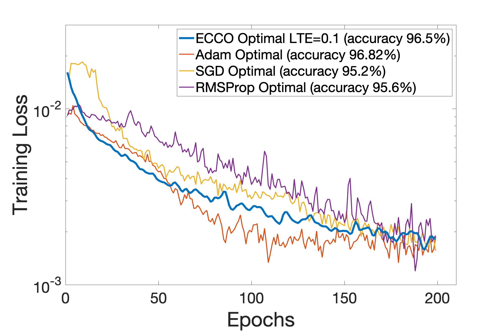
We next use ECCO on a machine learning application by training a neural network to classify MNIST data Deng 2012. See the Appendix G for details on this experiment. We compared first order ECCO (15) to stochastic gradient descent (SGD) with a fixed step size, Adam, and RMSProp⁷⁷ 7 A grid search was used to find hyperparameters for the comparison methods. See Appendix G.1 for details using a minibatch size of 1000. ECCO was adapted for a batch implementation in that every gradient was replaced with the sample gradient over the observed batch.

Figure 7 shows the results of training this experiment over 200 epochs; note that all four methods reach a similar training loss and have a similar test classification accuracy ($96\%$). See Appendix 2 for a discussion of wall clock times.

To test robustness, we perturbed the optimally tuned hyperparameter vectors within a normalized ball of radius $\varepsilon=0.1$. The hyperparameter values were sampled from a uniform distribution as $\tilde{\theta}\sim U(\max\{{\theta}^{*}-\frac{\varepsilon}{{\theta}^{*}},\underline{\theta}\},\min\{{\theta}^{*}+\frac{\varepsilon}{{\theta}^{*}},\bar{\theta}\})$, where ${\theta}^{*}$ was the optimal value as found by grid search. Note that this perturbation was bounded such that $\tilde{\theta}$ was always within the domain $[\underline{\theta},\bar{\theta}]$ of the hyperparameter. The network was then trained with $\tilde{\theta}$ and the test accuracy after 200 epochs was recorded in Figure 8. We find that while Adam, SGD, and RMSProp are disrupted by the hyperparameter perturbation, ECCO reliably trained in every test. In fact, we found $\eta$ could be changed by three orders of magnitude and still yield classification accuracies over 95%. See Appendix G.3 for more experiments.

These experiments demonstrate that ECCO can achieve convergence behavior on par with Adam without comparable computation and data requirements to select hyperparameters, i.e. cross-validation. This means ECCO is better than Adam at problem generalization and distribution shift.

References

- Aflak (2020) Aflak, O. Python neural networks, 2020. URL https://github.com/OmarAflak/python-neural-networks.
- Amid & Warmuth (2020) Amid, E. and Warmuth, M. K. Reparameterizing mirror descent as gradient descent. Advances in Neural Information Processing Systems, 33:8430–8439, 2020.
- Andrei (2004) Andrei, N. Gradient flow algorithm for unconstrained optimization. ICT Technical Report, 2004.
- Andrei (2008) Andrei, N. An unconstrained optimization test functions collection. Adv. Model. Optim, 10(1):147–161, 2008.
- Attouch & Cominetti (1996) Attouch, H. and Cominetti, R. A dynamical approach to convex minimization coupling approximation with the steepest descent method. Journal of Differential Equations, 128(2):519–540, 1996.
- Barrett & Dherin (2020) Barrett, D. G. and Dherin, B. Implicit gradient regularization. arXiv preprint arXiv:2009.11162, 2020.
- Behrman (1998) Behrman, W. An efficient gradient flow method for unconstrained optimization. stanford university, 1998.
- Boyd (2021) Boyd, S. Distributed optimization: Analysis and synthesis via circuits, 2021.
- Brown & Bartholomew-Biggs (1989) Brown, A. A. and Bartholomew-Biggs, M. C. Some effective methods for unconstrained optimization based on the solution of systems of ordinary differential equations. Journal of Optimization Theory and Applications, 62(2):211–224, 1989.
- Conn et al. (1991) Conn, A. R., Gould, N. I., and Toint, P. L. Convergence of quasi-newton matrices generated by the symmetric rank one update. Mathematical programming, 50(1-3):177–195, 1991.
- Cortés (2006) Cortés, J. Finite-time convergent gradient flows with applications to network consensus. Automatica, 42(11):1993–2000, 2006.
- Deng (2012) Deng, L. The mnist database of handwritten digit images for machine learning research. IEEE Signal Processing Magazine, 29(6):141–142, 2012.
- Desoer (2010) Desoer, C. A. Basic circuit theory. Tata McGraw-Hill Education, 2010.
- Fletcher (2013) Fletcher, R. Practical methods of optimization. John Wiley & Sons, 2013.
- Foster et al. (2022) Foster, E., Pandey, A., and Pileggi, L. Three-phase infeasibility analysis for distribution grid studies. Electric Power Systems Research, 212:108486, 2022. ISSN 0378-7796. doi: https://doi.org/10.1016/j.epsr.2022.108486. URL https://www.sciencedirect.com/science/article/pii/S0378779622006125.
- Franca et al. (2018) Franca, G., Robinson, D., and Vidal, R. Admm and accelerated admm as continuous dynamical systems. In International Conference on Machine Learning, pp. 1559–1567. PMLR, 2018.
- Helmke & Moore (2012) Helmke, U. and Moore, J. B. Optimization and dynamical systems. Springer Science & Business Media, 2012.
- Himmelblau (1972) Himmelblau, D. M. Applied Nonlinear Programming. McGraw-Hill, 1972. ISBN 0070289212.
- Hu & Lessard (2017) Hu, B. and Lessard, L. Dissipativity theory for nesterov’s accelerated method. In International Conference on Machine Learning, pp. 1549–1557. PMLR, 2017.
- Hustig-Schultz & Sanfelice (2019) Hustig-Schultz, D. M. and Sanfelice, R. G. A robust hybrid heavy ball algorithm for optimization with high performance. In 2019 American Control Conference (ACC), pp. 151–156. IEEE, 2019.
- Kingma & Ba (2014) Kingma, D. P. and Ba, J. Adam: A method for stochastic optimization. arXiv preprint arXiv:1412.6980, 2014.
- Latz (2021) Latz, J. Analysis of stochastic gradient descent in continuous time. Statistics and Computing, 31(4):1–25, 2021.
- Lin et al. (2016) Lin, P., Ren, W., and Farrell, J. A. Distributed continuous-time optimization: nonuniform gradient gains, finite-time convergence, and convex constraint set. IEEE Transactions on Automatic Control, 62(5):2239–2253, 2016.
- (24) Mike Engelhard. Ltspice. URL https://www.analog.com/en/design-center/design-tools-and-calculators/ltspice-simulator.html.
- Muehlebach & Jordan (2019) Muehlebach, M. and Jordan, M. A dynamical systems perspective on Nesterov acceleration. In Chaudhuri, K. and Salakhutdinov, R. (eds.), Proceedings of the 36th International Conference on Machine Learning, volume 97 of Proceedings of Machine Learning Research, pp. 4656–4662. PMLR, 09–15 Jun 2019. URL https://proceedings.mlr.press/v97/muehlebach19a.html.
- Muehlebach & Jordan (2021) Muehlebach, M. and Jordan, M. I. Optimization with momentum: Dynamical, control-theoretic, and symplectic perspectives. Journal of Machine Learning Research, 22(73):1–50, 2021.
- Murray et al. (2019) Murray, R., Swenson, B., and Kar, S. Revisiting normalized gradient descent: Fast evasion of saddle points. IEEE Transactions on Automatic Control, 64(11):4818–4824, 2019.
- Nagel & Rohrer (1971) Nagel, L. and Rohrer, R. Computer analysis of nonlinear circuits, excluding radiation (cancer). IEEE Journal of Solid-State Circuits, 6(4):166–182, 1971.
- Nagel (1975) Nagel, L. W. Spice2: A computer program to simulate semiconductor circuits. Ph. D. dissertation, University of California at Berkeley, 1975.
- (30) National Instrument Corporation. Multisimlive. URL https://www.multisim.com/.
- Peressini et al. (1988) Peressini, A. L., Sullivan, F. E., and Uhl Jr, J. J. The mathematics of nonlinear programming. Springer-Verlag, 1988.
- Pillage et al. (1995) Pillage, L., Rohrer, R., and Visweswariah, C. Electronic Circuit and System Simulation Methods. McGraw-Hill, 1995. ISBN 9780070501690. URL https://books.google.ca/books?id=uZZTAAAAMAAJ.
- Polyak & Shcherbakov (2017) Polyak, B. and Shcherbakov, P. Lyapunov functions: An optimization theory perspective. IFAC-PapersOnLine, 50(1):7456–7461, 2017.
- Rohrer & Nosrati (1981) Rohrer, R. and Nosrati, H. Passivity considerations in stability studies of numerical integration algorithms. IEEE transactions on circuits and systems, 28(9):857–866, 1981.
- Scieur et al. (2017) Scieur, D., Roulet, V., Bach, F., and d’Aspremont, A. Integration methods and optimization algorithms. Advances in Neural Information Processing Systems, 30, 2017.
- Surjanovic & Bingham (2013) Surjanovic, S. and Bingham, D. Usage statistics of content languages for websites, 2013. URL https://www.sfu.ca/˜ssurjano/optimization.html.
- Swenson et al. (2021) Swenson, B., Murray, R., Poor, H. V., and Kar, S. Distributed gradient flow: Nonsmoothness, nonconvexity, and saddle point evasion. IEEE Transactions on Automatic Control, 2021.
- Wilson (2018) Wilson, A. Lyapunov arguments in optimization. University of California, Berkeley, 2018.
- Wilson et al. (2021) Wilson, A. C., Recht, B., and Jordan, M. I. A lyapunov analysis of accelerated methods in optimization. Journal of Machine Learning Research, 22(113):1–34, 2021.
- Wolfe (1969) Wolfe, P. Convergence conditions for ascent methods. SIAM review, 11(2):226–235, 1969.
- Yuille & Kosowsky (1994) Yuille, A. L. and Kosowsky, J. Statistical physics algorithms that converge. Neural computation, 6(3):341–356, 1994.
Appendix A Proof of Theorem 1
Eq. (20) implies that the objective function is non-increasing along .