跳到论文正文
W Papers独立论文阅读器 arXiv:2211.08445 论文正文 计算阅读时间 · 0%
引用这篇论文根据当前论文元数据生成,正式投稿前建议核对。


License: CC BY 4.0
arXiv:2211.08445v2 [hep-ph] 24 Mar 2023

Constraints on the Doublet Left-Right Symmetric Model
from Higgs data

Siddhartha Karmakar Note: siddhartha.karmakar$_315$@tifr.res.in Affiliation: Department of Physics, Indian Institute of Technology Bombay,
Powai, Mumbai-400076, India
Affiliation: Department of Theoretical Physics, Tata Institute of Fundamental Research,
Colaba, Mumbai-400005, India
   Jai More Note: more.physics@gmail.com Affiliation: Department of Physics, Indian Institute of Technology Bombay,
Powai, Mumbai-400076, India
   Akhila Kumar Pradhan Note: akhilpradhan@iitb.ac.in Affiliation: Department of Physics, Indian Institute of Technology Bombay,
Powai, Mumbai-400076, India
   S. Uma Sankar Note: uma@phy.iitb.ac.in Affiliation: Department of Physics, Indian Institute of Technology Bombay,
Powai, Mumbai-400076, India
Abstract

We study the constraints on the doublet left-right symmetric model (DLRSM) arising due to the Higgs data. The S​U​(2)LSU(2)_{L} symmetry of this model is broken by three vacuum expectation values, κ1\kappa_{1}, κ2\kappa_{2} and vLv_{L}. Most studies of this model assume that the ratios r=κ2/κ1r=\kappa_{2}/\kappa_{1} and w=vL/κ1w=v_{L}/\kappa_{1} are very small. In this work, we study the constraints imposed on rr and ww by the Higgs data from LHC. We consider the most general scalar potential and calculate the masses of the CP-even scalars and the couplings of the lightest of these scalars to itself, to WW and ZZ gauge bosons and to the third generation quarks. We find that there is no lower bound on either rr or ww. Equating the mass of the lightest CP-even scalar to 125125 GeV leads to an upper limit w<6.7w<6.7. The requirement that the Yukawa coupling of the quarks to the Higgs bidoublet of the model should be perturbative yields the upper bounds r<0.8r<0.8 and w<3.5w<3.5. The Yukawa coupling of the bottom quark to the lightest CP-even scalar strongly disfavours value of r,w<0.1r,w<0.1 and shows a marked preference for values of w∼𝒪⁡(1)w\sim\mathcal{O}(1).

I Introduction

Left-right symmetric models, based on the symmetry group S​U​(2)L×S​U​(2)R×U​(1)B−LSU(2)_{L}\times SU(2)_{R}\times U(1)_{\rm B-L}, have been attractive candidates for physics beyond the standard model (SM) Pati:1974yy; Mohapatra:1974gc; Mohapatra:1974hk; Senjanovic:1975rk; Senjanovic:1978ev. In these models, the left-chiral fermions are doublets under S​U​(2)LSU(2)_{L} and singlets under S​U​(2)RSU(2)_{R}. The situation is reversed for the right-chiral fermions. The U​(1)B−LU(1)_{\rm B-L} hyper-charges of the fermions are fixed by the modified Gell-Mann-Nishijima formula connecting them to their respective electric charges. These models have been deployed to address numerous open problems of particle physics, such as neutrino mass generation, dark matter, unification of forces, etc.

The scalar sector of this model requires a minimum of three different Higgs multiplets. Fermion mass generation requires a scalar bidoublet Φ\Phi, which transforms as a doublet under both S​U​(2)LSU(2)_{L} and S​U​(2)RSU(2)_{R}. In addition, we need two more scalar multiplets to break the gauge symmetry of the model to U​(1)emU(1)_{\rm em} and to maintain the left-right symmetry of the Lagrangian. These additional scalars can be either S​U​(2)SU(2) doublets or triplets. In doublet left-right symmetric models (DLRSM), they are denoted as χL\chi_{L} (χR\chi_{R}) which is a doublet (singlet) under S​U​(2)LSU(2)_{L} and a singlet (doublet) under S​U​(2)RSU(2)_{R}. When the neutral component of χR\chi_{R} acquires the vacuum expectation value (vev) vRv_{R}, the symmetry of the model is broken to that of the SM. When the neutral components of χL\chi_{L} and Φ\Phi acquire vevs, the symmetry is finally broken to U​(1)emU(1)_{\rm em}. Since there is no evidence yet for any right-handed currents in weak interactions, the value of vRv_{R} has to be much greater than the vevs of χL\chi_{L} and Φ\Phi. If the additional scalars are S​U​(2)SU(2) triplets, the model is called triplet left-right symmetric model (TLRSM). In this model, it is possible to generate light Majorana masses for neutrinos, through both type-I and type-II see-saw mechanisms. The constraints on the scalar sector of this model are qualitatively different from those of DLRSM. In this work, we confine our attention to DLRSM.

The minimal form of DLRSM was originally discussed in ref. Senjanovic:1978ev. Ref. Babu:1988qv extended this model by adding a singly-charged S​U​(2)SU(2) singlet complex scalar so that small neutrino masses can be generated at one-loop level by the Zee mechanism Zee:1980ai. Such a scalar mixes with the charged scalars in DLRSM. The details of this mixing are constrained from the neutrino oscillation data Babu:2020bgz, flavour violating decays of charged leptons FileviezPerez:2017zwm, and collider searches for RH neutrinos FileviezPerez:2016erl.

It is an interesting question to ask what the dominant source of electroweak symmetry breaking (EWSB) in DLRSM is: whether it is the vev vLv_{L} of the doublet χL\chi_{L} or the vevs κ1\kappa_{1} and κ2\kappa_{2} of the bidoublet Φ\Phi. Most models, based on left-right symmetry, assume the latter to be the case. By considering the bounds from perturbative unitarity of scalar and gauge boson scattering and the electroweak precision data, ref. Bernard:2020cyi showed that both the above possibilities are allowed. It means there is no hierarchy between vLv_{L} and κ1\kappa_{1}, κ2\kappa_{2}. Most left-right symmetric models also assume κ2≪κ1\kappa_{2}\ll\kappa_{1}. It will be interesting to see what bounds the data imposes on this hierarchy. The purpose of the current study is to analyse the pattern of EWSB in the simplest DLRSM in light of Higgs data and theoretical arguments such as perturbativity, unitarity, and boundedness from below.

In sec. II we introduce our notations and discuss the key features of the different sectors of DLRSM. In sec. III we mention the bounds from perturbativity, unitarity, and boundedness from below. A convenient and minimal basis of quartic parameters have been introduced in sec. IV. Salient features of the model in light of Higgs data are presented in sec. V. This section also discusses the validity of the assumption of hierarchy in the vevs vL,κ2≪κ1v_{L},\kappa_{2}\ll\kappa_{1} as a function of the values of the quartic couplings in the model. We make our concluding remarks in sec. VI.

II The Doublet Left-Right Symmetric Model: Essentials and Notations

DLRSM is based on the gauge symmetry S​U​(3)C×S​U​(2)L×S​U​(2)R×U​(1)B−LSU(3)_{C}\times SU(2)_{L}\times SU(2)_{R}\times U(1)_{B-L}. The fermion content of the model is given below, where the parenthesis contain the quantum numbers of the fermions under each of the sub-groups of the gauge group,

QL\displaystyle Q_{L} =(uLdL)∼(3,2,1,1/3),QR=(uRdR)∼(3,1,2,1/3),\displaystyle=\begin{pmatrix}u_{L}\\ d_{L}\\ \end{pmatrix}\sim(3,2,1,1/3),\hskip 28.45274ptQ_{R}=\begin{pmatrix}u_{R}\\ d_{R}\\ \end{pmatrix}\sim(3,1,2,1/3),
LL\displaystyle L_{L} =(νLeL)∼(1,2,1,−1),LR=(νReR)∼(1,1,2,−1).\displaystyle=\begin{pmatrix}\nu_{L}\\ e_{L}\\ \end{pmatrix}\sim(1,2,1,-1),\hskip 34.1433ptL_{R}=\begin{pmatrix}\nu_{R}\\ e_{R}\\ \end{pmatrix}\sim(1,1,2,-1). (1)

For any left-right symmetric model, parity is truly manifest as a symmetry, making the Lagrangian symmetric under transformations QL↔QRQ_{L}\leftrightarrow Q_{R}, LL↔LRL_{L}\leftrightarrow L_{R}. Note that the model necessarily contains a right-handed neutrino νR\nu_{R}, which is required to complete the lepton doublet. Both νL\nu_{L} and νR\nu_{R} receive Majorana masses if DLRSM is extended with additional scalars FileviezPerez:2017zwm or fermions Brdar:2018sbk. In our work, we do not include these additional fields.

II.1 The scalar potential

The scalar sector consists of a complex bidoublet and two doublets with the following charges under the aforementioned gauge group

Φ=(ϕ10ϕ2+ϕ1−ϕ20)∼(1,2,2,0),χL=(χL+χL0)∼(1,2,1,1),χR=(χR+χR0)∼(1,1,2,1),\displaystyle\Phi=\begin{pmatrix}\phi_{1}^{0}&\phi_{2}^{+}\\ \phi_{1}^{-}&\phi_{2}^{0}\\ \end{pmatrix}\sim(1,2,2,0),\hskip 5.0pt\chi_{L}=\begin{pmatrix}\chi_{L}^{+}\\ \chi_{L}^{0}\\ \end{pmatrix}\sim(1,2,1,1),\hskip 5.0pt\chi_{R}=\begin{pmatrix}\chi_{R}^{+}\\ \chi_{R}^{0}\\ \end{pmatrix}\sim(1,1,2,1)\,\,,

with the vev structure

⟨Φ⟩=12​(κ100κ2),⟨χL⟩=12​(0vL),⟨χR⟩=12​(0vR).\displaystyle\langle\Phi\rangle=\frac{1}{\sqrt{2}}\begin{pmatrix}\kappa_{1}&0\\ 0&\hskip 8.53581pt\ \kappa_{2}\\ \end{pmatrix}\,,\hskip 19.91692pt\langle\chi_{L}\rangle=\frac{1}{\sqrt{2}}\begin{pmatrix}0\\ v_{L}\\ \end{pmatrix}\,,\hskip 19.91692pt\langle\chi_{R}\rangle=\frac{1}{\sqrt{2}}\begin{pmatrix}0\\ v_{R}\\ \end{pmatrix}\,. (2)

The spontaneous breaking of S​U​(2)R×U​(1)B−L→U​(1)YSU(2)_{R}\times U(1)_{B-L}\rightarrow U(1)_{Y} is driven by the vev of the doublet χR\chi_{R} whereas the EWSB is triggered by the three vevs κ1\kappa_{1}, κ2\kappa_{2}, and vLv_{L}. The last three vevs are constrained by κ12+κ22+vL2=v2\kappa_{1}^{2}+\kappa_{2}^{2}+v_{L}^{2}=v^{2}, where v=246v=246 GeV. For later use, it is convenient to introduce the ratios r=κ2/κ1r=\kappa_{2}/\kappa_{1} and w=vL/κ1w=v_{L}/\kappa_{1}. The vevs of the scalars must have the hierarchy vR≫vv_{R}\gg v, which ensures that the gauge bosons of S​U​(2)RSU(2)_{R} are much heavier than the weak gauge bosons. The Yukawa couplings of the bidoublet with fermions lead to fermion masses and mixings. The details of these couplings will be discussed later in sec. II.4.

The most general, CP-conserving, renormalizable Higgs potential involving Φ,χL\Phi,\chi_{L} and χR\chi_{R} fields is given by

V\displaystyle V =\displaystyle= V2+V3+V4,\displaystyle V_{2}+V_{3}+V_{4},
V2\displaystyle V_{2} =\displaystyle= −μ12​Tr​(Φ†​Φ)−μ22​[Tr​(Φ~​Φ†)+Tr​(Φ~†​Φ)]−μ32​[χL†​χL+χR†​χR],\displaystyle-\mu_{1}^{2}\text{Tr}(\Phi^{\dagger}\Phi)-\mu_{2}^{2}\ [\text{Tr}(\tilde{\Phi}\Phi^{\dagger})+\text{Tr}(\tilde{\Phi}^{\dagger}\Phi)]-\mu_{3}^{2}\ [\chi_{L}^{\dagger}\chi_{L}+\chi_{R}^{\dagger}\chi_{R}]\,\,,
V3\displaystyle V_{3} =\displaystyle= μ4​[χL†​Φ​χR+χR†​Φ†​χL]+μ5​[χL†​Φ~​χR+χR†​Φ~†​χL],\displaystyle\mu_{4}\ [\chi_{L}^{\dagger}\Phi\chi_{R}+\chi_{R}^{\dagger}\Phi^{\dagger}\chi_{L}]+\mu_{5}\ [\chi_{L}^{\dagger}\tilde{\Phi}\chi_{R}+\chi_{R}^{\dagger}\tilde{\Phi}^{\dagger}\chi_{L}]\,\,,
V4\displaystyle V_{4} =\displaystyle= λ1​Tr​(Φ†​Φ)2+λ2​[Tr​(Φ~​Φ†)2+Tr​(Φ~†​Φ)2]+λ3​Tr​(Φ~​Φ†)​Tr​(Φ~†​Φ)\displaystyle\lambda_{1}\text{Tr}(\Phi^{\dagger}\Phi)^{2}+\lambda_{2}\ [\text{Tr}(\tilde{\Phi}\Phi^{\dagger})^{2}+\text{Tr}(\tilde{\Phi}^{\dagger}\Phi)^{2}]+\lambda_{3}\text{Tr}(\tilde{\Phi}\Phi^{\dagger})\,\text{Tr}(\tilde{\Phi}^{\dagger}\Phi) (3)
+λ4​Tr​(Φ†​Φ)​[Tr​(Φ~​Φ†)+Tr​(Φ~†​Φ)]+ρ1​[(χL†​χL)2+(χR†​χR)2]+ρ2​χL†​χL​χR†​χR\displaystyle+\lambda_{4}\text{Tr}(\Phi^{\dagger}\Phi)\,[\text{Tr}(\tilde{\Phi}\Phi^{\dagger})+\text{Tr}(\tilde{\Phi}^{\dagger}\Phi)]+\rho_{1}\ [(\chi_{L}^{\dagger}\chi_{L})^{2}+(\chi_{R}^{\dagger}\chi_{R})^{2}]+\rho_{2}\ \chi_{L}^{\dagger}\chi_{L}\chi_{R}^{\dagger}\chi_{R}
+α1Tr(Φ†Φ)[χL†χL+χR†χR]+{α2[χL†χLTr(Φ~Φ†)+χR†χRTr(Φ~†Φ)]+h.c.}\displaystyle+\alpha_{1}\text{Tr}(\Phi^{\dagger}\Phi)[\chi_{L}^{\dagger}\chi_{L}+\chi_{R}^{\dagger}\chi_{R}]+\Big\{\alpha_{2}\ [\chi_{L}^{\dagger}\chi_{L}\text{Tr}(\tilde{\Phi}\Phi^{\dagger})+\chi_{R}^{\dagger}\chi_{R}\text{Tr}(\tilde{\Phi}^{\dagger}\Phi)]+{\rm h.c.}\Big\}
+α3​[χL†​Φ​Φ†​χL+χR†​Φ†​Φ​χR]+α4​[χL†​Φ~​Φ~†​χL+χR†​Φ~†​Φ~​χR].\displaystyle+\alpha_{3}\ [\chi_{L}^{\dagger}\ \Phi\Phi^{\dagger}\chi_{L}+\chi_{R}^{\dagger}\Phi^{\dagger}\Phi\chi_{R}]+\alpha_{4}\ [\chi_{L}^{\dagger}\ \tilde{\Phi}\tilde{\Phi}^{\dagger}\chi_{L}+\chi_{R}^{\dagger}\tilde{\Phi}^{\dagger}\tilde{\Phi}\chi_{R}]\,\,.

Here all the couplings can be made real by appropriate field redefinitions.

The following conditions minimize the potential

∂V∂κ1=∂V∂κ2=∂V∂vL=∂V∂vR=0.\frac{\partial V}{\partial\kappa_{1}}=\frac{\partial V}{\partial\kappa_{2}}=\frac{\partial V}{\partial v_{L}}=\frac{\partial V}{\partial v_{R}}=0\,\,. (4)

We utilize these conditions to replace the four mass parameters μ12,μ22,μ32\mu_{1}^{2},\mu_{2}^{2},\mu_{3}^{2} and μ5\mu_{5} by the vevs and quartic couplings,

μ12\displaystyle\mu_{1}^{2} =\displaystyle= 12​(r2−1)​(κ12​(w2​((r2−1)​α1+r2​α3−α4)+2​(r2−1)​((r2+1)​λ1+2​r​λ4))CLOSE\displaystyle\frac{1}{2(r^{2}-1)}\Bigg(\kappa_{1}^{2}\Big(w^{2}((r^{2}-1)\alpha_{1}+r^{2}\alpha_{3}-\alpha_{4})+2(r^{2}-1)((r^{2}+1)\lambda_{1}+2r\lambda_{4})\Big)
OPEN+2​2​r​vR​w​μ4+vR2​((r2−1)​α1+r2​α3−α4+2​w2​ρ12)),\displaystyle+2\sqrt{2}rv_{R}w\mu_{4}+v_{R}^{2}\Big((r^{2}-1)\alpha_{1}+r^{2}\alpha_{3}-\alpha_{4}+2w^{2}\rho_{12}\Big)\Bigg)\,\,,
μ22\displaystyle\mu_{2}^{2} =\displaystyle= 14​(r2−1)​(κ12​(w2​(r2−1)​α2−w2​r​α34+2​(r2−1)​(2​r​λ23+(r2+1)​λ4))CLOSE\displaystyle\frac{1}{4(r^{2}-1)}\Bigg(\kappa_{1}^{2}\Big(w^{2}(r^{2}-1)\alpha_{2}-w^{2}r\alpha_{34}+2(r^{2}-1)(2r\lambda_{23}+(r^{2}+1)\lambda_{4})\Big)
OPEN−2​(r2+1)​vR​w​μ4+vR2​((r2−1)​α2−r​α34−2​w2​ρ12)),\displaystyle-\sqrt{2}(r^{2}+1)v_{R}w\mu_{4}+v_{R}^{2}\Big((r^{2}-1)\alpha_{2}-r\alpha_{34}-2w^{2}\rho_{12}\Big)\Bigg)\,\,,
μ32\displaystyle\mu_{3}^{2} =\displaystyle= 12​κ12​((r2+1)​α1+2​r​α2+r2​α3+α4+2​w2​ρ1)+vR2​ρ1,\displaystyle\frac{1}{2}\kappa_{1}^{2}((r^{2}+1)\alpha_{1}+2r\alpha_{2}+r^{2}\alpha_{3}+\alpha_{4}+2w^{2}\rho_{1})+v_{R}^{2}\rho_{1}\,\,,
μ5\displaystyle\mu_{5} =\displaystyle= −r​μ4−2​vR​w​ρ12.\displaystyle-r\mu_{4}-\sqrt{2}v_{R}w\rho_{12}\,\,. (5)

Here ρ12=ρ2/2−ρ1\rho_{12}=\rho_{2}/2-\rho_{1}, α34=α3−α4\alpha_{34}=\alpha_{3}-\alpha_{4}, and λ23=2​λ2+λ3\lambda_{23}=2\lambda_{2}+\lambda_{3}. From the definition of rr and ww, we note that κ12​(1+r2+w2)=v2\kappa_{1}^{2}(1+r^{2}+w^{2})=v^{2}. That is, the value of κ1\kappa_{1} is fixed for a given rr and ww. Thus the parameters of the DLRSM scalar sector are

{λ1,2,3,4,α1,2,3,4,ρ1,2,μ4,r,w,vR}.\displaystyle\{\lambda_{1,2,3,4},\alpha_{1,2,3,4},\rho_{1,2},\mu_{4},r,w,v_{R}\}\,\,. (6)

Among these, the only dimensionful parameter is μ4\mu_{4}. For most of the following discussions, we will either set it to zero or restrict it to μ4≲vR\mu_{4}\lesssim v_{R}.

II.2 The gauge sector

The charged gauge boson mass matrix in this model is

ℒm​a​s​s⊃(WL+WR+)​(gL24​(vL2+κ12+κ22)−12​gL​gR​κ1​κ2−12​gL​gR​κ1​κ2gR24​(vR2+κ12+κ22))​(WL−WR−).\displaystyle\mathcal{L}_{mass}\supset\begin{pmatrix}W_{L}^{+}&W_{R}^{+}\end{pmatrix}\begin{pmatrix}\frac{g_{L}^{2}}{4}(v_{L}^{2}+\kappa_{1}^{2}+\kappa_{2}^{2})&-\frac{1}{2}g_{L}g_{R}\kappa_{1}\kappa_{2}\\ -\frac{1}{2}g_{L}g_{R}\kappa_{1}\kappa_{2}&\frac{g_{R}^{2}}{4}(v_{R}^{2}+\kappa_{1}^{2}+\kappa_{2}^{2})\end{pmatrix}\begin{pmatrix}W_{L}^{-}\\ W_{R}^{-}\\ \end{pmatrix}. (7)

Here gL⁡(R)g_{L(R)} are the gauge couplings associated with S​U​(2)L⁡(R)SU(2)_{L(R)}. The physical charged gauge bosons have masses

mW1,22=18​(gL2​v2+gR2​V2∓(gL2​v2−gR2​V2)2+16​gL2​gR2​κ12​κ22),\displaystyle m^{2}_{W_{1,2}}=\frac{1}{8}\Big(g_{L}^{2}v^{2}+g_{R}^{2}V^{2}\mp\sqrt{(g_{L}^{2}v^{2}-g_{R}^{2}V^{2})^{2}+16g_{L}^{2}g_{R}^{2}\kappa_{1}^{2}\kappa_{2}^{2}}\Big)\,\,\,, (8)

where W1±W_{1}^{\pm} is close to the SM W±W^{\pm} boson and W2W_{2} has mass of the order of vRv_{R}. The mixing between WL±W_{L}^{\pm} and WR±W_{R}^{\pm} given by

(WL±WR±)=(cos⁡ξ−sin⁡ξsin⁡ξcos⁡ξ)​(W1±W2±),\displaystyle\begin{pmatrix}W_{L}^{\pm}\\ W_{R}^{\pm}\\ \end{pmatrix}=\begin{pmatrix}\cos\xi&-\sin\xi\\ \sin\xi&\cos\xi\end{pmatrix}\begin{pmatrix}W_{1}^{\pm}\\ W_{2}^{\pm}\\ \end{pmatrix},

where

tan⁡ξ=4​gL​gR​κ1​κ2gL2​v2−gR2​V2−(gL2​v2−gR2​V2)2+16​gL2​gR2​κ12​κ22.\displaystyle\tan\xi=\frac{4g_{L}g_{R}\kappa_{1}\kappa_{2}}{g_{L}^{2}v^{2}-g_{R}^{2}V^{2}-\sqrt{(g_{L}^{2}v^{2}-g_{R}^{2}V^{2})^{2}+16g_{L}^{2}g_{R}^{2}\kappa_{1}^{2}\kappa_{2}^{2}}}\,\,\,. (9)

Here, we adhere to the definitions, v2=κ12+κ22+vL2v^{2}=\kappa_{1}^{2}+\kappa_{2}^{2}+v_{L}^{2} and V2=κ12+κ22+vR2V^{2}=\kappa_{1}^{2}+\kappa_{2}^{2}+v_{R}^{2}. In the limit κ1,κ2,vL≪vR\kappa_{1},\kappa_{2},v_{L}\ll v_{R} and gL=gRg_{L}=g_{R}, the mixing angle becomes ξ≃−2κ1κ2/vR2\xi\simeq-2\kappa_{1}\kappa_{2}/v_{R}^{2}.

In a similar fashion, the neutral gauge boson mass matrix can be written as

ℒm​a​s​s⊃18​(WL​μ3WR​μ3Bμ)​(gL2​v2−gL​gR​κ+2−gL​gB​L​vL2gR2​V2−gR​gB​L​vR2gB​L2​(vL2+vR2))​(WL​μ3WR​μ3Bμ),\displaystyle\mathcal{L}_{mass}\supset\frac{1}{8}\begin{pmatrix}W^{3}_{L\mu}&W^{3}_{R\mu}&B_{\mu}\end{pmatrix}\begin{pmatrix}g_{L}^{2}v^{2}&-g_{L}g_{R}\kappa_{+}^{2}&-g_{L}g_{BL}v_{L}^{2}\\ &g_{R}^{2}V^{2}&-g_{R}g_{BL}v_{R}^{2}\\ &&g_{BL}^{2}(v_{L}^{2}+v_{R}^{2})\end{pmatrix}\begin{pmatrix}W^{3}_{L\mu}\\ W^{3}_{R\mu}\\ B_{\mu}\end{pmatrix}\,\,,

with the mass eigenvalues

mZ1,Z22\displaystyle m^{2}_{Z_{1},Z_{2}} =\displaystyle= 18​(gL2​v2+gR2​V2+gB​L2​(vL2+vR2)CLOSE\displaystyle\frac{1}{8}\Big(g_{L}^{2}v^{2}+g_{R}^{2}V^{2}+g_{BL}^{2}(v_{L}^{2}+v_{R}^{2})
OPEN∓(gL2​v2+gR2​V2+gB​L2​(vL2+vR2))2+4​(gL2​gR2+gL2​gB​L2+gR2​gB​L2)​(κ+4−v2​V2)),\displaystyle\mp\sqrt{(g_{L}^{2}v^{2}+g_{R}^{2}V^{2}+g_{BL}^{2}(v_{L}^{2}+v_{R}^{2}))^{2}+4(g_{L}^{2}g_{R}^{2}+g_{L}^{2}g_{BL}^{2}+g_{R}^{2}g_{BL}^{2})(\kappa_{+}^{4}-v^{2}V^{2})}\Big)\,\,,

where κ+2=κ12+κ22\kappa_{+}^{2}=\kappa_{1}^{2}+\kappa_{2}^{2} and gB​Lg_{BL} is the gauge coupling of U​(1)B−LU(1)_{B-L}. The lighter boson Z1Z_{1} is close to the SM ZZ boson and the heavier boson Z2Z_{2} has a mass of order vRv_{R}. The exact expressions for the mass eigenstates in terms of the gauge eigenstates are given in Appendix A.

In the limit κ1,κ2,vL≪vR\kappa_{1},\kappa_{2},v_{L}\ll v_{R} and gL=gR=gg_{L}=g_{R}=g the mixing reduces to Dev:2016dja

(AμZ1​μZ2​μ)=(sWcW​sYcW​cY−cWsW​sYsW​cY0cYsY)​(WL​μ3WR​μ3Bμ),\displaystyle\begin{pmatrix}A_{\mu}\\ Z_{1\mu}\\ Z_{2\mu}\end{pmatrix}=\begin{pmatrix}s_{W}&c_{W}s_{Y}&c_{W}c_{Y}\\ -c_{W}&s_{W}s_{Y}&s_{W}c_{Y}\\ 0&c_{Y}&s_{Y}\end{pmatrix}\begin{pmatrix}W^{3}_{L\mu}\\ W^{3}_{R\mu}\\ B_{\mu}\end{pmatrix}, (12)

where

sW\displaystyle s_{W} ≡\displaystyle\equiv sin⁡θW=gB​Lg2+2​gB​L2,cW≡cos⁡θW=g2+gB​L2g2+2​gB​L2,\displaystyle\sin\theta_{W}=\frac{g_{BL}}{\sqrt{g^{2}+2g_{BL}^{2}}}\,\,,\,\,\,\,\,c_{W}\equiv\cos\theta_{W}=\sqrt{\frac{g^{2}+g_{BL}^{2}}{g^{2}+2g_{BL}^{2}}}\,\,,
sY\displaystyle s_{Y} ≡\displaystyle\equiv sin⁡θY=gB​Lg2+gB​L2,cY≡cos⁡θY=gg2+gB​L2.\displaystyle\sin\theta_{Y}=\frac{g_{BL}}{\sqrt{g^{2}+g_{BL}^{2}}}\,\,,\,\,\,\,\,c_{Y}\equiv\cos\theta_{Y}=\frac{g}{\sqrt{g^{2}+g_{BL}^{2}}}\,\,. (13)

In the remainder of the paper we will assume manifest LR symmetry in the gauge sector leading to gL=gR=gg_{L}=g_{R}=g.

If we retain only vR2v_{R}^{2} terms in eqs. (8) and (), we find mW2=g​vR/2m_{W_{2}}=gv_{R}/2 and mZ2=mW2/cos⁡θYm_{Z_{2}}=m_{W_{2}}/\cos\theta_{Y}. The present experimental lower limits on charged heavy gauge boson is mW′≥6m_{W^{\prime}}\geq 6  TeV ATLAS:2019lsy, obtained under the assumption that fermions couple to W′W^{\prime} and to the usual WW with the same strength. This assumption is certainly valid for manifest DLRSM. Since vR≈2​mW2/gv_{R}\approx 2m_{W_{2}}/g, we must have vR∼20v_{R}\sim 20  TeV to satisfy the experimental lower bound on mW2m_{W_{2}}. The experimental lower bound on neutral heavy gauge boson is mZ′≥5.1m_{Z^{\prime}}\geq 5.1  TeV ATLAS:2019erb; CMS:2021ctt, which again is obtained under the assumption that the fermions couple to Z′Z^{\prime} and to the usual ZZ with the same strength. Such an assumption is approximately true for manifest DLRSM. Since the predicted value of mZ2m_{Z_{2}} is greater than the predicted value of mW2m_{W_{2}}, the lower bound on mZ2m_{Z_{2}} is automatically satisfied if the lower bound on mW2m_{W_{2}} is satisfied. Our numerical calculations give the values mW2=6.5m_{W_{2}}=6.5  TeV and mZ2=7.7m_{Z_{2}}=7.7  TeV for vR=20v_{R}=20  TeV. When the S​U​(2)LSU(2)_{L} breaking vevs, κ1,κ2\kappa_{1},\kappa_{2} and vLv_{L} are varied subject to the constraint κ12+κ22+vL2=v2\kappa_{1}^{2}+\kappa_{2}^{2}+v_{L}^{2}=v^{2}, the changes in mW2m_{W_{2}} and mZ2m_{Z_{2}} are less than 1%1\%.

II.3 CP-even neutral scalars

The experiments at LHC have measured the mass of the Higgs boson and its couplings to gauge bosons and fermions. They have also set lower limits on masses of heavy neutral and charged scalars. The aim of this work is to utilize the Higgs boson measurements to constrain the parameters of DLRSM. So we study the CP-even neutral scalars of DLRSM in detail. For completeness, we have included the masses of CP-odd neutral scalars and charged scalars in Appendix A.

The gauge and physical bases for the CP-even neutral scalars are X=(ϕ1​r0,ϕ2​r0,χL​r0,χR​r0)X=(\phi_{1r}^{0},\phi_{2r}^{0},\chi_{Lr}^{0},\chi_{Rr}^{0}) and Xph=(h,H1,H2,H3)X_{\text{ph}}=(h,H_{1},H_{2},H_{3}) respectively. Here hh is the lightest CP-even scalar with mass of the order of vv and Hi​(i=1,2,3)H_{i}\,(i=1,2,3) are heavier scalars with masses of the order of vRv_{R}. It is expected that the properties of hh will be very similar to those of SM Higgs boson.

The mass matrix for scalars in the gauge basis is denoted by M2M^{2}. It can be decomposed in powers of vRv_{R} which enables the use of perturbation theory due to the hierarchy of scales κ1,κ2,vL≪vR\kappa_{1},\kappa_{2},v_{L}\ll v_{R},

M2=(M2​(0)​vR2+M2​(1)​vR+M2​(2)),\displaystyle M^{2}=\Big(M^{2\,(0)}v_{R}^{2}+M^{2\,(1)}v_{R}+M^{2\,(2)}\Big)\,\,\,, (14)

where M2​(0)M^{2\,(0)}, M2​(1)M^{2\,(1)} and M2​(2)M^{2\,(2)} are three symmetric matrices. The eigenvalues of this matrix must be positive, because they represent the masses of the scalars. The explicit forms of these symmetric components are

(M2​(2))11\displaystyle\big(M^{2\,(2)}\big)_{11} =\displaystyle= 12​κ12​(w2​(α1+α4)+2​(3+r2)​λ1+4​r​(r​λ23+3​λ4)),\displaystyle\frac{1}{2}\kappa_{1}^{2}(w^{2}(\alpha_{1}+\alpha_{4})+2(3+r^{2})\lambda_{1}+4r(r\lambda_{23}+3\lambda_{4}))\,\,,
(M2​(2))12\displaystyle\big(M^{2\,(2)}\big)_{12} =\displaystyle= 12​κ12​(w2​α2+4​r​(λ1+2​λ23)+6​(r2+1)​λ4),\displaystyle\frac{1}{2}\kappa_{1}^{2}(w^{2}\alpha_{2}+4r(\lambda_{1}+2\lambda_{23})+6(r^{2}+1)\lambda_{4})\,\,,
(M2​(2))13\displaystyle\big(M^{2\,(2)}\big)_{13} =\displaystyle= w​κ12​(α1+r​α2+α4),(M2​(0))14=−r​w​κ1​μ42,\displaystyle w\kappa_{1}^{2}(\alpha_{1}+r\alpha_{2}+\alpha_{4})\,\,,\,\,\,\,\,\,\big(M^{2\,(0)}\big)_{14}=-\frac{rw\kappa_{1}\mu_{4}}{\sqrt{2}}\,\,,
(M2​(2))22\displaystyle\big(M^{2\,(2)}\big)_{22} =\displaystyle= 12​κ12​(w2​(α1+α3)+2​(3​r2+1)​λ1+4​(λ23+3​r​λ4)),\displaystyle\frac{1}{2}\kappa_{1}^{2}(w^{2}(\alpha_{1}+\alpha_{3})+2(3r^{2}+1)\lambda_{1}+4(\lambda_{23}+3r\lambda_{4}))\,\,,
(M2​(2))23\displaystyle\big(M^{2\,(2)}\big)_{23} =\displaystyle= w​κ12​(α2+r⁡(α1+α3)),(M2​(0))24=w​κ1​μ42,\displaystyle w\kappa_{1}^{2}(\alpha_{2}+r(\alpha_{1}+\alpha_{3}))\,\,,\,\,\big(M^{2\,(0)}\big)_{24}=\frac{w\kappa_{1}\mu_{4}}{\sqrt{2}}\,\,,
(M2​(2))33\displaystyle\big(M^{2\,(2)}\big)_{33} =\displaystyle= 12​κ12​((r2+1)​α1+2​r​α2+r2​α3+α4+6​w2​ρ1),(M2​(2))34=0,\displaystyle\frac{1}{2}\kappa_{1}^{2}((r^{2}+1)\alpha_{1}+2r\alpha_{2}+r^{2}\alpha_{3}+\alpha_{4}+6w^{2}\rho_{1})\,\,,\,\,\,\,\,\big(M^{2\,(2)}\big)_{34}=0\,\,,
(M2​(2))44\displaystyle\big(M^{2\,(2)}\big)_{44} =\displaystyle= 12​κ12​((r2+1)​α1+2​r​α2+r2​α3+α4+w2​ρ2),\displaystyle\frac{1}{2}\kappa_{1}^{2}((r^{2}+1)\alpha_{1}+2r\alpha_{2}+r^{2}\alpha_{3}+\alpha_{4}+w^{2}\rho_{2})\,\,\,, (15)
M2​(1)\displaystyle M^{2\,(1)} =\displaystyle= (2​r​w​μ41−r2−(r2+1)​w​μ42​(1−r2)−r​μ42κ1​((α1+r​α2+α4)−w2​ρ12)2​r​w​μ41−r2μ42κ1​(α2+r⁡(α1+α3))0w​κ1​(ρ1+ρ2/2)0),\displaystyle\begin{pmatrix}\frac{\sqrt{2}rw\mu_{4}}{1-r^{2}}&-\frac{(r^{2}+1)w\mu_{4}}{\sqrt{2}(1-r^{2})}&-\frac{r\mu_{4}}{\sqrt{2}}&\kappa_{1}((\alpha_{1}+r\alpha_{2}+\alpha_{4})-w^{2}\rho_{12})\\ &\frac{\sqrt{2}rw\mu_{4}}{1-r^{2}}&\frac{\mu_{4}}{\sqrt{2}}&\kappa_{1}(\alpha_{2}+r(\alpha_{1}+\alpha_{3}))\\ &&0&w\kappa_{1}(\rho_{1}+\rho_{2}/2)\\ &&&0\end{pmatrix}\,\,\,, (16)
M2​(0)\displaystyle M^{2\,(0)} =\displaystyle= (r2​α34+2​w2​ρ122​(1−r2)r⁡(α34+2​w2​ρ12)2​(1−r2)−w​ρ120α34+2​w2​ρ122​(1−r2)00ρ1202​ρ1),\displaystyle\begin{pmatrix}\frac{r^{2}\alpha_{34}+2w^{2}\rho_{12}}{2(1-r^{2})}&\frac{r(\alpha_{34}+2w^{2}\rho_{12})}{2(1-r^{2})}&-w\rho_{12}&0\\ &\frac{\alpha_{34}+2w^{2}\rho_{12}}{2(1-r^{2})}&0&0\\ &&\rho_{12}&0\\ &&&2\rho_{1}\end{pmatrix}\,\,\,\,, (17)

where, for convenience, only the upper halves of the matrices M2​(1)M^{2\,(1)} and M2​(0)M^{2\,(0)} are displayed in eqs. (16) and (17) respectively.

Since the smallest eigenvalue of M2M^{2} must be of order v2v^{2}, its expression must not contain any positive powers of vRv_{R}. Hence both M2​(0)M^{2\,(0)} and M2​(1)M^{2\,(1)} must have zero as their smallest eigenvalues. The other three eigenvalues of M2M^{2} correspond to (mass)2 of heavy CP-even scalars. This requires the non-zero eigenvalues of M2​(0)M^{2\,(0)} to be positive.

We aim to calculate the smallest eigenvalue of M2M^{2} using perturbation theory. First we apply a similarity transformation on M2M^{2}, using the orthogonal matrix Babu:2020bgz which diagonalizes M2​(0)M^{2\,(0)},

OI=(1krkwk0−r1+r2−11+r200−wk​1+r2−r​wk​1+r2−1+r2k00001),\displaystyle O_{I}=\begin{pmatrix}\frac{1}{k}&\frac{r}{k}&\frac{w}{k}&0\\ -\frac{r}{\sqrt{1+r^{2}}}&-\frac{1}{\sqrt{1+r^{2}}}&0&0\\ -\frac{w}{k\sqrt{1+r^{2}}}&-\frac{rw}{k\sqrt{1+r^{2}}}&-\frac{\sqrt{1+r^{2}}}{k}&0\\ 0&0&0&1\end{pmatrix}\,\,\,\,, (18)

where k2=1+r2+w2k^{2}=1+r^{2}+w^{2}. In the rotated basis the mass-squared matrix has the form

M~2=(M~2​(0)​vR2+M~2​(1)​vR+M~2​(2)).\begin{split}\tilde{M}^{2}=\Big(\tilde{M}^{2\,(0)}v_{R}^{2}+\tilde{M}^{2\,(1)}v_{R}+\tilde{M}^{2\,(2)}\Big)\end{split}\,\,. (19)

It is straight forward to check that both M~2​(0)\tilde{M}^{2\,(0)} and M~2​(1)\tilde{M}^{2\,(1)} have one zero eigenvalue. The positivity of the non-zero eigenvalues of M~2​(0)\tilde{M}^{2\,(0)} leads to the following constraints on the quartic couplings

2​ρ12=ρ2−2​ρ1>0​and​α34=α3−α4>0.2\rho_{12}=\rho_{2}-2\rho_{1}>0~~{\rm and}~~\alpha_{34}=\alpha_{3}-\alpha_{4}>0\,\,. (20)

Using non-degenerate perturbation theory, the smallest eigenvalue of M2M^{2}, which we take to be Higgs boson mass mh2m_{h}^{2}, is found to be

mh2\displaystyle m_{h}^{2} =\displaystyle= (M~2​(2))11−[(M~2​(1))14]22​ρ1\displaystyle(\tilde{M}^{2\,(2)})_{11}-\frac{[(\tilde{M}^{2\,(1)})_{14}]^{2}}{2\rho_{1}}\,\,\, (21)
=\displaystyle= κ122​(1+r2+w2)×\displaystyle\frac{\kappa_{1}^{2}}{2(1+r^{2}+w^{2})}\times
(4​(λ1​(r2+1)2+4​r​(λ4​(r2+1)+r​λ23)+w2​(α124+r2​(α1+α3)+α2​r)+ρ1​w4)CLOSE\displaystyle\Bigg(4\Big(\lambda_{1}(r^{2}+1)^{2}+4r(\lambda_{4}(r^{2}+1)+r\lambda_{23})+w^{2}(\alpha_{124}+r^{2}(\alpha_{1}+\alpha_{3})+\alpha_{2}r)+\rho_{1}w^{4}\Big)
OPEN−1ρ1​(α124+r2​(α1+α3)+α2​r+2​ρ1​w2)2),\displaystyle\,\,\,\,\,\,\,-\frac{1}{\rho_{1}}(\alpha_{124}+r^{2}(\alpha_{1}+\alpha_{3})+\alpha_{2}r+2\rho_{1}w^{2})^{2}\Bigg),

where α124=α1+r​α2+α4\alpha_{124}=\alpha_{1}+r\alpha_{2}+\alpha_{4} Bernard:2020cyi. Since mh2m_{h}^{2} should be positive, the second term in eq. (21) must always be less than the first. Thus the Higgs mass constraint imposes a rather strong restriction on the quartic couplings of DLRSM.

However, it has to be noted that for some specific set of values of quartic couplings, the assumptions of non-degenerate perturbation theory will not be valid. In these scenarios, the smallest eigenvalue of M2M^{2} matrix may differ significantly from the value given by the expression in eq. (21). We are interested in exploring the constraints on full parameter space of the quartic couplings. Therefore, we diagonalize the mass matrix numerically to avoid the pitfalls of possible near degeneracies of the diagonal elements of M2M^{2} matrix. As discussed in the introduction, we need a vRv_{R} of about 2020 TeV to satisfy the experimental lower bound on heavy charged gauge boson mass. Hence, we set vR=20v_{R}=20 TeV in our numerical work, which also ensures that κ12,κ22,vL2≪vR2\kappa_{1}^{2},\kappa_{2}^{2},v_{L}^{2}\ll v_{R}^{2}.

DLRSM contains the following extra scalars compared to the SM:

  • •

    three CP-even scalars, labelled H1,2,3H_{1,2,3} earlier in this section,

  • •

    two CP-odd scalars, labelled A1A_{1} and A2A_{2},

  • •

    two pairs of charged scalars, labelled H1±H_{1}^{\pm} and H2±H_{2}^{\pm}.

Among these, the CP-even scalar H3H_{3} has some peculiar properties. Its predominant component is the S​U​(2)RSU(2)_{R} scalar χR0\chi_{R}^{0} and its mass is given by mH32≈2​ρ1​vR2m^{2}_{H_{3}}\approx 2\rho_{1}v_{R}^{2}. Its couplings to SM fermions and gauge bosons are highly suppressed. Hence mass constraints on neutral scalars from neither flavour changing neutral interactions (FCNI) nor direct searches are applicable to H3H_{3}. In principle, its mass can be quite low Dev:2016dja, much lower than those of H1H_{1} and H2H_{2}. The rest of the extra scalars can have significant coupling to SM fermions and gauge bosons and hence all the experimental constraints on heavy scalar masses will be applicable to them.

The gauge and the mass eigenstates of the neutral scalars are related by

Xph=UT​X,UT​M2​U=M2 diag.\displaystyle X_{\text{ph}}=U^{T}X,\,\,\,\,\,\,\,\,\,\,\,\,\,U^{T}M^{2}U=M^{\text{2 diag}}\,\,. (22)

The coupling of scalars in the gauge basis to W1W_{1} boson is

ℒ⊃12​g2​((κ1−2​cξ​sξ​κ2)​ϕ1​r0+(κ2−2​cξ​sξ​κ1)​ϕ2​r0+vL​cξ2​χL​r0+vR​sξ2​χR​r0)​W1​μ+​W1−μ,\displaystyle\mathcal{L}\supset\frac{1}{2}g^{2}\,\big((\kappa_{1}-2c_{\xi}s_{\xi}\kappa_{2})\phi^{0}_{1r}+(\kappa_{2}-2c_{\xi}s_{\xi}\kappa_{1})\phi^{0}_{2r}+v_{L}c_{\xi}^{2}\chi_{Lr}^{0}+v_{R}s_{\xi}^{2}\chi_{Rr}^{0}\big)\,W^{+}_{1\mu}\,W^{-\mu}_{1}\,\,\,,

where ξ\xi is the mixing angle between WL,RW_{L,R} given by eq. (9). Transforming the scalar gauge eigenstates to mass eigenstates, we find the coupling multiplier for the 3-point interaction of hh to W1W_{1} bosons to be

κW=ch​W1​W1ch​W​WSM=1k​((1−2​cξ​sξ​r)​U11+(r−2​cξ​sξ)​U21+w​cξ2​U31+vRκ1​sξ2​U41),\displaystyle\kappa_{W}=\frac{c_{hW_{1}W_{1}}}{c_{hWW}^{\text{SM}}}=\frac{1}{k}\Big((1-2c_{\xi}s_{\xi}r)U_{11}+(r-2c_{\xi}s_{\xi})U_{21}+wc_{\xi}^{2}U_{31}+\frac{v_{R}}{\kappa_{1}}s_{\xi}^{2}U_{41}\Big), (24)

where we expressed the DLRSM coupling in the form of a ratio to the corresponding SM coupling. This makes is easier to compare our model calculations with the experimental results of Higgs boson couplings because they are given in the form of such ratios. Similarly, the coupling of scalars in gauge basis to the Z1Z_{1}-boson is

ℒ⊃g24​(cW+sW​sY)2​(κ1​ϕ1​r0+κ2​ϕ2​r0+vL​χL​r0)​Z1​μ​Z1μ,\displaystyle\mathcal{L}\supset\frac{g^{2}}{4}\,(c_{W}+s_{W}s_{Y})^{2}(\kappa_{1}\phi^{0}_{1r}+\kappa_{2}\phi^{0}_{2r}+v_{L}\chi^{0}_{Lr})\,Z_{1\mu}\,Z^{\mu}_{1}\,\,\,, (25)

which gives

κZ=g2​(g2+2​gB​L2)(g2+g′2)​(g2+gB​L2)​1k​(U11+r​U21+w​U31).\displaystyle\kappa_{Z}=\frac{g^{2}(g^{2}+2g_{BL}^{2})}{(g^{2}+g^{\prime 2})(g^{2}+g_{BL}^{2})}\,\frac{1}{k}\,(U_{11}+rU_{21}+wU_{31})\,\,. (26)

Here g′g^{\prime} is the gauge coupling of U​(1)YU(1)_{Y} of SM. We use gB​L=g​g′/(g2−g′2)1/2g_{BL}=gg^{\prime}/(g^{2}-g^{\prime 2})^{1/2} which reduces the fraction involving the gauge couplings in eq. (26) to unity Georgi:1977wk.

Triple Higgs (h3)(h^{3}) vertex in this model is given by

ch3\displaystyle c_{h^{3}} =\displaystyle= κ12​(2​(λ1+r​λ4)​U113+2​(r​λ1+λ4)​U213+2​w​ρ1​U313+2​(r⁡(λ1+4​λ2+2​λ3)+3​λ4)​U112​U21CLOSE\displaystyle\frac{\kappa_{1}}{2}\Big(2(\lambda_{1}+r\lambda_{4})U_{11}^{3}+2(r\lambda_{1}+\lambda_{4})U_{21}^{3}+2w\rho_{1}U_{31}^{3}+2(r(\lambda_{1}+4\lambda_{2}+2\lambda_{3})+3\lambda_{4})U_{11}^{2}U_{21} (27)
+2​(λ1+4​λ2+2​λ3+3​λ4​r)​U11​U212+w⁡(α1+α4)​U112​U31+(α1+r​α2+α4)​U11​U312\displaystyle\hskip 20.0pt+2(\lambda_{1}+4\lambda_{2}+2\lambda_{3}+3\lambda_{4}r)U_{11}U_{21}^{2}+w(\alpha_{1}+\alpha_{4})U_{11}^{2}U_{31}+(\alpha_{1}+r\alpha_{2}+\alpha_{4})U_{11}U_{31}^{2}
OPEN+w⁡(α1+α3)​U212​U31+(α2+r⁡(α1+α3))​U21​U312),\displaystyle\hskip 20.0pt+w(\alpha_{1}+\alpha_{3})U_{21}^{2}U_{31}+(\alpha_{2}+r(\alpha_{1}+\alpha_{3}))U_{21}U_{31}^{2}\Big)\,\,\,,

with the corresponding coupling multiplier being κh=ch3/ch3SM\kappa_{h}=c_{h^{3}}/c_{h^{3}}^{\textrm{SM}} where ch3SM=mh2/2​vc_{h^{3}}^{\textrm{SM}}=m_{h}^{2}/2v.

II.4 The fermion sector

The fermions obtain masses through their Yukawa couplings to the bidoublet. For the quark sector, these couplings are

ℒY​u​k⊃−Q¯L​i​(yi​j​Φ+y~i​j​Φ~)​QR​j+h.c.,\displaystyle\mathcal{L}_{Yuk}\supset-\bar{Q}_{Li}(y_{ij}\Phi+\tilde{y}_{ij}\tilde{\Phi})Q_{Rj}+h.c.\,\,, (28)

which lead to the following mass terms

ℒm⊃−U¯L​i′​(MU)i​j​UR​j′−D¯L​i′​(MD)i​j​DR​j′+h.c..\displaystyle\mathcal{L}_{m}\supset-\bar{U}^{\prime}_{Li}(M_{U})_{ij}U^{\prime}_{Rj}-\bar{D}^{\prime}_{Li}(M_{D})_{ij}D^{\prime}_{Rj}+h.c.\,\,. (29)

Here U′≡(u′,c′,t′)U^{\prime}\equiv(u^{\prime},c^{\prime},t^{\prime}) and D′≡(d′,s′,b′)D^{\prime}\equiv(d^{\prime},s^{\prime},b^{\prime}) are up- and down-type quarks in the gauge basis. The mass matrices MU⁡(D)M_{U(D)}, in general, are complex and arbitrary

MU=12​(κ1​y+κ2​y~),MD=12​(κ2​y+κ1​y~).\displaystyle M_{U}=\frac{1}{\sqrt{2}}(\kappa_{1}y+\kappa_{2}\tilde{y}),\,\,\,\,M_{D}=\frac{1}{\sqrt{2}}(\kappa_{2}y+\kappa_{1}\tilde{y})\,\,.

They must be diagonalized to identify the quark mass eigenstates. Interactions of the gauge eigenstates of the neutral CP-even scalars to quarks are given by Deshpande:1990ip

ℒN\displaystyle\mathcal{L}_{N} ⊃\displaystyle\supset κ12​κ−2u¯L​i((ϕ10−rϕ20∗)M^u+(−rϕ10+ϕ20∗)VLCKMM^dVRCKM†)uR​j\displaystyle\frac{\kappa_{1}}{\sqrt{2}\,\kappa_{-}^{2}}\,\bar{u}_{Li}\Bigg((\phi^{0}_{1}-r\phi^{0*}_{2})\hat{M}_{u}+(-r\phi^{0}_{1}+\phi_{2}^{0*})V_{L}^{\text{CKM}}\,\hat{M}_{d}\,V_{R}^{\text{CKM}\dagger}\Bigg)u_{Rj} (30)
+κ12​κ−2d¯L​i((ϕ10∗−rϕ20)M^d+(−rϕ10∗+ϕ20)VLCKM†M^uVRCKM)dR​j+h.c.,\displaystyle+\frac{\kappa_{1}}{\sqrt{2}\,\kappa_{-}^{2}}\,\bar{d}_{Li}\Bigg((\phi^{0*}_{1}-r\phi^{0}_{2})\hat{M}_{d}+(-r\phi^{0*}_{1}+\phi_{2}^{0})V_{L}^{\text{CKM}\dagger}\,\hat{M}_{u}\,V_{R}^{\text{CKM}}\Bigg)d_{Rj}+h.c.\,\,,

where κ−2=κ12−κ22=(1−r2)​κ12\kappa_{-}^{2}=\kappa_{1}^{2}-\kappa_{2}^{2}=(1-r^{2})\kappa_{1}^{2} and M^u⁡(d)\hat{M}_{u(d)} is the diagonal up (down)-type quark matrix** * In the gauge basis of the scalars, the Yukawa sector of DLRSM is the same as a triplet left-right symmetric model of ref. Deshpande:1990ip.. As we consider a scalar sector that conserves CP at the tree-level, manifest left-right symmetry holds in the quark sector, i.e., VRCKM=VLCKMV_{R}^{\text{CKM}}=V_{L}^{\text{CKM}}. We use the Wolfenstein parametrization of the CKM matrix with best-fit values of relevant parameters pdg:ckm

A=0.79,λ=0.2265,ρ¯=0.141,η¯=0.357.\displaystyle A=0.79,\,\,\,\lambda=0.2265,\,\,\,\bar{\rho}=0.141,\,\,\,\bar{\eta}=0.357\,\,.

Using eqs. (22) and (30) we obtain the couplings of CP-even scalars with quarks. We find that the couplings of fermions to the lightest scalar hh are essentially flavour diagonal with small flavour violating couplings of the order of v2/vR2v^{2}/v_{R}^{2}. The heavier scalars, with masses of the order of vRv_{R}, have flavour violating couplings in general. For vR=20v_{R}=20 TeV, the amplitudes of FCNI are below the experimental upper bounds. The coupling of the CP-even lightest scalar to third generation quarks are given as

ch​t​t​(h​b​b)=κ12​κ−2((U11−rU21)mt⁡(b)+(U21−rU11)(VLCKMM^d⁡(u)VRCKM†)33),\displaystyle c_{htt\,(hbb)}=\frac{\kappa_{1}}{\sqrt{2}\,\kappa_{-}^{2}}\,\Big((U_{11}-rU_{21})m_{t(b)}+(U_{21}-rU_{11})(V_{L}^{\text{CKM}}\,\hat{M}_{d(u)}\,V_{R}^{\text{CKM}\dagger})_{33}\Big), (31)

which can be used to obtain the coupling multipliers κt\kappa_{t} and κb\kappa_{b}, as κf=ch​f​f/ch​f​fSM\kappa_{f}=c_{hff}/c_{hff}^{\text{SM}}, where ch​f​fSM=mf/vc_{hff}^{\text{SM}}=m_{f}/v and f=tf=t or bb.

III Theoretical constraints

Here we briefly discuss the theoretical constraints on DLRSM, such as perturbativity of the quartic and Yukawa couplings, perturbative unitarity of gauge boson scattering, and boundedness of the scalar potential from below.

III.1 Perturbativity of the quartic and Yukawa couplings

Perturbativity bounds on the quadratic couplings dictate αi,λi,ρj≲4​π\alpha_{i},\lambda_{i},\rho_{j}\lesssim 4\pi, where i=1,2,3,4i=1,2,3,4 and j=1,2j=1,2. Moreover, we also assume μ4≲vR\mu_{4}\lesssim v_{R}.

Perturbativity of the Yukawa couplings yy and y~\tilde{y} appearing in eq. (28) pose a strong bound on the r−wr-w plane. In the limit (VL,RCKM)33∼1\Big(V_{L,R}^{\text{CKM}}\Big)_{33}\sim 1,

y33=2​(1+r2+w2)1/2v⁡(1−r2)​(mt−r​mb),\displaystyle y_{33}=\frac{\sqrt{2}(1+r^{2}+w^{2})^{1/2}}{v(1-r^{2})}\,(m_{t}-r\,m_{b})\,\,\,,
y~33=2​(1+r2+w2)1/2v⁡(1−r2)​(mb−r​mt).\displaystyle\tilde{y}_{33}=\frac{\sqrt{2}(1+r^{2}+w^{2})^{1/2}}{v(1-r^{2})}\,(m_{b}-r\,m_{t})\,\,\,. (32)

From these equations, we note that y33≃1y_{33}\simeq 1 and y~33≃1/40\tilde{y}_{33}\simeq 1/40 for very small values of rr and ww. The perturbativity requirement of y33<(4​π)1/2y_{33}<(4\pi)^{1/2} leads to strong upper limits r≲0.8r\lesssim 0.8, and w≲3.5w\lesssim 3.5. The perturbativity requirement of y~33\tilde{y}_{33} gives comparatively weaker constraints. These constraints are shown in fig. 1.

Refer to caption
Figure 1: The black and red contours represent the values of y33y_{33} and y~33\tilde{y}_{33} respectively.

III.2 Perturbative unitarity of gauge boson scattering

The condition of unitarity of the 2→22\to 2 scattering of the gauge degrees of freedom impose certain constraints on the masses and couplings of the new scalars. Some of these constraints are superseded by perturbativity for r<1r<1. But the following conditions must be satisfied at 𝒪⁡(κ1/vR)\mathcal{O}(\kappa_{1}/v_{R}) Bernard:2020cyi

0<ρ1<8​π3,or,​mH32vR2\displaystyle 0<\rho_{1}<\frac{8\pi}{3}\,,\,\,\text{or,}\,\,\frac{m_{H_{3}}^{2}}{v_{R}^{2}} <\displaystyle< 16​π3,\displaystyle\frac{16\pi}{3}\,\,\,,
(cH3)2k4​mH32vR2\displaystyle\frac{(c_{H_{3}})^{2}}{k^{4}}\,\frac{m^{2}_{H_{3}}}{v_{R}^{2}} <\displaystyle< 16​π3,\displaystyle\frac{16\pi}{3}\,\,\,,
2​w2k2​∑i=1,2Fi2​mHi±2vR2+cH3k2​mH32vR2\displaystyle 2\frac{w^{2}}{k^{2}}\sum_{i=1,2}F_{i}^{2}\frac{m^{2}_{H^{\pm}_{i}}}{v_{R}^{2}}+\frac{c_{H_{3}}}{k^{2}}\frac{m^{2}_{H_{3}}}{v_{R}^{2}} <\displaystyle< 16​π,\displaystyle 16\pi\,\,\,,
2​w2k2​∑i=1,2Si2​mHi±2vR2+cH3k2​mH32vR2\displaystyle 2\frac{w^{2}}{k^{2}}\sum_{i=1,2}S_{i}^{2}\frac{m^{2}_{H^{\pm}_{i}}}{v_{R}^{2}}+\frac{c_{H_{3}}}{k^{2}}\frac{m^{2}_{H_{3}}}{v_{R}^{2}} <\displaystyle< 16​π,\displaystyle 16\pi\,\,\,, (33)

where the expressions for cH3c_{H_{3}}, SiS_{i} and FiF_{i}, in terms of the parameters of the Higgs potential, are given in ref. Bernard:2020cyi.

III.3 Boundedness from below

Criteria for boundedness from below of the DLRSM scalar potential has been studied in the literature utilising the copositivity criteria Chakrabortty:2013zja; Chakrabortty:2016wkl and gauge orbit formulation Chauhan:2019fji; Frank:2021ekj; Kannike:2021fth. These studies used different simplified forms of the potential. We have derived the criteria for boundedness from below for the most general potential given by eq. (3). These are described in Appendix B.

III.4 Custodial symmetry breaking

Some key constraints on the extended scalar sectors arise from the measurement of the ρ\rho parameter, which quantifies the breaking of the custodial symmetry of the scalar potential in the SM. The tree-level contribution to ρ=mW12/mZ12cosθW2\rho=m_{W_{1}}^{2}/m_{Z_{1}}^{2}\cos\theta_{W}^{2} in the DLRSM appears at the order (v/vR)2(v/v_{R})^{2} Bernard:2020cyi.

IV A convenient parametrization of the quartic couplings

The model contains ten quartic couplings overall, four λ\lambdas, four α\alphas and two ρ\rhos. These couplings have to satisfy various inequalities arising from the theoretical constraints discussed in the previous section and the positivity of CP-even scalar masses. There is an inequality on the ratio x=λ2/λ4x=\lambda_{2}/\lambda_{4} arising from boundedness of the scalar potential. As shown in Appendix B, this inequality is of the form 8​x​(1−x)>08x(1-x)>0. For positive xx, this translates into 0.25≤x≤0.850.25\leq x\leq 0.85.

We are interested in how the Higgs data constrain ranges of rr and ww. In studying these constraints, in principle, the ten quartic couplings should be allowed to take ten independent values, subject to the inequalities mentioned above. However, a study with ten free parameters does not give a good insight into various inter-relations. To gain an insight as to how the data constrains rr and ww, we pick a simplified set of three quartic couplings λ0,α0\lambda_{0},\alpha_{0} and ρ1\rho_{1}. We fix the ten quartic couplings by using relations

{λ1=λ3=λ4=λ0,x=λ2λ4,α1=α2=α4=α0,p=α3α4−1,q=ρ22​ρ1−1}.\displaystyle\{\lambda_{1}=\lambda_{3}=\lambda_{4}=\lambda_{0},\,\,\,x=\frac{\lambda_{2}}{\lambda_{4}},\,\,\,\alpha_{1}=\alpha_{2}=\alpha_{4}=\alpha_{0},\,\,\,p=\frac{\alpha_{3}}{\alpha_{4}}-1,\,\,\,q=\frac{\rho_{2}}{2\rho_{1}}-1\}. (34)

The set of parameters {λ0,α0,ρ1,x,p,q,r,w,vR}\{\lambda_{0},\alpha_{0},\rho_{1},x,p,q,r,w,v_{R}\} together with vv provides the most minimal simplified basis to describe the scalar potential of the model. From now on we refer to this as the ‘simple’ basis, as opposed to the ‘generic’ basis where all the λ\lambdas and all the α\alphas are taken to be independent. We note that, both in the simple basis and in the generic basis, pp and qq parameters need to be positive.

V Constraints from the Higgs data

In sec. III, we derived the upper bounds on rr and ww from theoretical constraints. In this section, we investigate the constraints on these parameters coming from the Higgs data. We first do this study in the simple basis of the DLRSM quartic couplings to see the pattern of allowed regions in the r−wr-w plane. We then re-do the study in the generic basis to see what changes, if any, are there in our results.

V.1 Constraints in the simple basis

In the simple basis, there are eight parameters, three quartic couplings, the three ratios pp, qq and xx, the coupling of three scalar multiplets μ4\mu_{4}, and vRv_{R}. In our calculations, we fix the values of vR=20v_{R}=20 TeV. We vary the other parameters randomly and identify regions in the parameter space which satisfy the experimental constraints from the Higgs data.

The mass of the lightest Higgs scalar depends strongly on the quartic couplings λ\lambda, as shown in eq. (21). Hence, the constraint on mhm_{h} will be satisfied only for a limited range of values of λ0\lambda_{0}. Therefore, in choosing random values of this parameter, we limit ourselves to a restricted range. For specific values of α0\alpha_{0}, ρ1\rho_{1}, xx, pp, and qq, we solve eq. (21) and obtain a solution for λ0\lambda_{0} which we label Λ0\Lambda_{0}. To maximize the number of points satisfying the mhm_{h} constraint, we choose random values of λ0\lambda_{0} in the limited range

λ0=(1+y)​Λ0​with​y∈[−0.1,0.1].\displaystyle\lambda_{0}=(1+y)\,\Lambda_{0}\,\,{\rm with}\,\,y\in[-0.1,0.1]. (35)

This choice ensures that most of the random points satisfy the Higgs mass constraint and enables us to study how the constraints from the κ\kappa factors restrict the parameters of the model.

The random values of xx and yy are picked in linear scale in their respective ranges. For the other parameters, the random values are picked in a log scale, in the ranges specified below:

α1,2,4≡α0∈[10−3,4​π],ρ1∈[0.1,8​π/3],μ4∈[10−2,1]×vR.\alpha_{1,2,4}\equiv\alpha_{0}\in[10^{-3},4\pi],\,\,\rho_{1}\in[0.1,8\pi/3],\,\,\mu_{4}\in[10^{-2},1]\times v_{R}. (36)

This choice of using logarithmic scale, leads to very small values of the parameters being as likely as the values of the order 11. Of the two ratios, pp and qq, we hold qq fixed at q=1q=1 but consider four different values for pp, varying from a low value of 0.020.02 to a high value of 55.

Observable Observed value
mhm_{h} (125.38±0.14)(125.38\pm 0.14) GeV CMS:2020xrn
κW\kappa_{W} 1.05±0.061.05\pm 0.06 ATLAS:2020qdt
κZ\kappa_{Z} 0.96±0.070.96\pm 0.07 CMS:2020gsy
κh\kappa_{h} [−2.3,10.3][-2.3,10.3] at 95%95\% CL ATLAS:2019pbo
κt\kappa_{t} 1.01±0.111.01\pm 0.11 CMS:2020gsy
κb\kappa_{b} 0.98−0.13+0.140.98^{+0.14}_{-0.13} ATLAS:2020qdt
Table 1: Experimental values of the Higgs mass and coupling multipliers used in our calculations.
Refer to caption
Refer to caption
Refer to caption
Refer to caption
Figure 2: Allowed points on the rr-ww plane with random values of α1,2,4=α0∈[10−3,4​π]\alpha_{1,2,4}=\alpha_{0}\in[10^{-3},4\pi], λ1,3,4=λ0∈[10−3,4​π]\lambda_{1,3,4}=\lambda_{0}\in[10^{-3},4\pi], x=λ2/λ0∈[0.25,0.85]x=\lambda_{2}/\lambda_{0}\in[0.25,0.85], ρ1∈[0.1,4​π]\rho_{1}\in[0.1,4\pi] for four different values of pp. The values of qq and vRv_{R} are held fixed at q=1q=1 and vR=20v_{R}=20 TeV respectively. Light blue points satisfy mhm_{h}, κh\kappa_{h}, κW\kappa_{W}, κZ\kappa_{Z} and κt\kappa_{t} constraints and theoretical bounds. Red points satisfy κb\kappa_{b} constraint also and dark blue points satisfy the additional constraint mH1>15m_{H_{1}}>15 TeV.

For each random point, we numerically calculate the lightest Higgs mass mhm_{h} and the coupling parameters κW\kappa_{W}, κZ\kappa_{Z}, κh\kappa_{h}, κt\kappa_{t} and κb\kappa_{b} and demand that they should match the corresponding experimentally measured values, listed in Table 1. The results of our calculation are displayed in fig. 2. The light blue dots satisfy the theoretical bounds and the constraints from mhm_{h}, κh\kappa_{h}, κW\kappa_{W}, κZ\kappa_{Z} and κt\kappa_{t}. By considering these constraints individually, it was found the κh\kappa_{h} constraint rules out a significant number of points allowed by the mhm_{h} constraint. The κW\kappa_{W}, κZ\kappa_{Z} and κt\kappa_{t} constraints are satisfied by all the points which satisfy mhm_{h} and κh\kappa_{h} constraints. The red dots satisfy the additional constraint from κb\kappa_{b} parameter. The κb\kappa_{b} constraint leads to a drastic reduction in the number of allowed points for low values of pp. In particular, for p=0.02p=0.02, very low values of rr and ww are ruled out. As the value of pp increases, points of low rr and low ww become allowed but there is a clear preference for larger values of ww as long as p≤0.1p\leq 0.1. Only for p≥1p\geq 1, the distribution of allowed points is uniform over the full range of rr and ww. This means we need to have α3\alpha_{3} at least twice as large as the other α\alpha s, if the usual assumption vL,κ2≪κ1v_{L},\kappa_{2}\ll\kappa_{1} is to hold.

The reason for this strong influence of κb\kappa_{b} can be understood from eqs. (17) and (31). In the expression for κb\kappa_{b} in eq. (31), the second term is proportional to mtm_{t}. If the CP-even scalar mixing matrix element U21U_{21} is not negligible, this second term can lead to a large value of κb\kappa_{b}. The dominant contribution to mH12m_{H_{1}}^{2} comes from vR2​M222​(0)=vR2​[p​α3+2​w2​ρ12]/[2​(1−r2)]v_{R}^{2}M^{2(0)}_{22}=v_{R}^{2}\,[p\,\alpha_{3}+2w^{2}\rho_{12}]/[2(1-r^{2})] in eq. (17). If M222​(0)M^{2(0)}_{22} is too small, there will be a significant mixing between hh and H1H_{1}, i.e., U21U_{21} is not negligible and the predicted κb\kappa_{b} will deviate significantly from 11. A large value for M222​(0)M^{2(0)}_{22} can be obtained for r≃1r\simeq 1, independent of the values of pp and ww, but this violates the perturbativity of the Yukawa coupling y33y_{33} and is not allowed. For moderate values of rr, either pp or ww (or both) must take reasonably large values to satisfy the constraint on κb\kappa_{b}. We see this feature illustrated in fig. 2 where small values of ww are ruled out by the κb\kappa_{b} constraint when pp is small but become progressively more allowed as pp becomes larger.

In addition to the constraint from the measured parameters listed in Table 1, there is an important indirect bound on the masses of heavy CP-even scalars from flavour changing neutral interactions. The requirement that these interactions be adequately suppressed leads to a strong bound Zhang:2007da

mH1≥15​TeV.\displaystyle m_{H_{1}}\geq 15\,{\rm TeV}. (37)

In fig. 2, dark blue dots represent the points which satisfy this additional constraint also. For p≤1p\leq 1, the blue dots are bunched towards values of w≥0.6w\geq 0.6. The few points of low ww, which occur for r≃1r\simeq 1 are ruled out by the constraint r≤0.8r\leq 0.8, arising from the perturbativity bound on the Yukawa coupling y33y_{33}. Therefore, the bound on mH1m_{H_{1}} strongly prefers that vev of χL\chi_{L} has a significant influence on the breaking of S​U​(2)LSU(2)_{L}. For very large values of p≥5p\geq 5, we see a reasonably large number of blue dots in the region of low rr and low ww. For example, in fig. 2 (d), the range r∈[10−3,10−2]r\in[10^{-3},10^{-2}] and w∈[10−6,10−3]w\in[10^{-6},10^{-3}] contains ∼14%\sim 14\% of the total number of points allowed from the measurements of mhm_{h}, κh\kappa_{h}, κt\kappa_{t}, κb\kappa_{b}, and mH1>15m_{H_{1}}>15 TeV. These points correspond to larger values of ρ1≳1\rho_{1}\gtrsim 1 which push ρ2>4\rho_{2}>4 making it relatively large. That is, the usual assumption vL,κ2≪κ1v_{L},\kappa_{2}\ll\kappa_{1} holds, only if the quartic couplings ρ1\rho_{1} and ρ2\rho_{2} take moderately large values.

In the expression for κh\kappa_{h} in eq. (27), the terms proportional to ww always make a positive contribution to the value of κh\kappa_{h}. Hence, the experimental upper limit on κh\kappa_{h} affects the region of large ww significantly. In future, if this upper limit is improved to κh<2\kappa_{h}<2, values of w>1w>1 will be ruled out. Hence the points satisfying all the constraints (dark blue points of fig. 2) will occur only for very large values of p∼5p\sim 5 with allowed values of w<0.5w<0.5.

We now briefly discuss what happens when the ratio qq is allowed to deviate from 11. From eq. (17), we see that leading contribution to the mass of one of the heavier Higgses is ρ12​vR2=ρ1​q​vR2\rho_{12}v_{R}^{2}=\rho_{1}qv_{R}^{2}. Hence, very small values of qq will not satisfy mH1>15m_{H_{1}}>15 TeV constraint whereas larger values of qq will violate unitarity bounds. These two constraints together restrict qq to the range 0.01≤q≤40.01\leq q\leq 4. The constraints from mhm_{h}, κh\kappa_{h}, κW\kappa_{W}, κZ\kappa_{Z}, κt\kappa_{t} and κb\kappa_{b} are unaffected by changes in the value of qq. As a result, the points satisfying all the constraints (dark blue points of fig. (2)) are depleted overall if qq deviates from 1. For the extreme allowed values of qq, i.e., q∼0.01q\sim 0.01 and q∼4q\sim 4, mH1>15m_{H_{1}}>15 TeV is more likely to be satisfied for w≳1w\gtrsim 1. As mentioned above, these extreme values will be ruled out if κh\kappa_{h} is measured to be less than 22.

In the analysis above, the constraints on mhm_{h} and mH1m_{H_{1}} were discussed thoroughly. Here we briefly comment on the masses of the additional scalars in the model. The algebraic expressions for their masses are given in Appendix A. We find that mH1,mA1m_{H_{1}},m_{A_{1}} and mH1±m_{H_{1}^{\pm}} are all highly degenerate with their masses differing by less than 1%1\%, for the values of quartic couplings which satisfy all the experimental constraint listed in Table 1. We also find that the masses of other scalars, mH2,mA2m_{H_{2}},m_{A_{2}} and mH2±m_{H_{2}}^{\pm} are similarly degenerate but at a higher values compared to mH1m_{H_{1}}.

V.2 A strong upper limit on vLv_{L} from Higgs mass

Refer to caption
Figure 3: Allowed points on the rr-ww plane for λi,αi∈[10−3,1]\lambda_{i},\alpha_{i}\in[10^{-3},1], ρ1∈[0.1,8​π/3]\rho_{1}\in[0.1,8\pi/3], and ρ2∈[0.1,4​π]\rho_{2}\in[0.1,4\pi]. The light blue points satisfy mhm_{h}, κW\kappa_{W}, κZ\kappa_{Z}, κh\kappa_{h} and κt\kappa_{t} constraints and theoretical bounds. The red points satisfy κb\kappa_{b} constraint in addition and the dark blue points satisfy mH1>15m_{H_{1}}>15 TeV constraint. All the allowed points are below the red line, which represents the analytical upper limit of ww. The black solid lines represent contours of Yukawa couplings y33y_{33}.

As mentioned earlier, the parameter space with w≳1w\gtrsim 1 is of special interest. It was seen in fig. 2 that there is a strong upper bound on ww arising from the measurement of mhm_{h}. In the simple basis eq. (21) takes the form

mh2=v2(1+r2+w2)2​[2​(8​λ2​r2+λ0​(1+r2)4)−α02​(2+r⁡(2+(2+p)​r))22​ρ1].\displaystyle m_{h}^{2}=\frac{v^{2}}{(1+r^{2}+w^{2})^{2}}\Big[2\big(8\lambda_{2}r^{2}+\lambda_{0}(1+r^{2})^{4}\big)-\frac{\alpha_{0}^{2}(2+r(2+(2+p)r))^{2}}{2\rho_{1}}\Big]\,\,. (38)

In the limit α0→0\alpha_{0}\rightarrow 0 and r→1r\rightarrow 1, imposing the perturbativity bounds λ0,λ2<4​π\lambda_{0},\lambda_{2}<4\pi leads to the upper limit w<6.81w<6.81. Demand of boundedness from below requires λ2<0.85​λ0\lambda_{2}<0.85\,\lambda_{0}, which in turn, slightly reduces the upper limit to w<6.71w<6.71. The upper limit can also be obtained as a function of rr, wmax​(r)≃a+b​r+c​r2w_{\text{max}}(r)\simeq a+br+cr^{2}, where a=2.9332a=2.9332, b=4.3535b=4.3535, and c=−0.4755c=-0.4755. If the maximum values of the couplings α0\alpha_{0} and λ0,2\lambda_{0,2} are taken to be 11 instead of 4​π4\pi, the upper limit reduces to wmax∼2.8w_{\text{max}}\sim 2.8 at r∼1r\sim 1. In fig. 3 we have illustrated this analytical bound on top of a random scan over α0,λ0∈[10−3,1]\alpha_{0},\lambda_{0}\in[10^{-3},1] which shows that all the allowed points are below the limit imposed by the Higgs mass constraint of eq. (38). Note that, the perturbativity limit on y33y_{33} is stronger than the Higgs data for r≳0.5r\gtrsim 0.5. As a result, the effective upper limit on ww as a function of rr is set by the interplay of mhm_{h} and perturbativity of y33y_{33}.

V.3 Constraints in the generic basis

In the generic basis, each quartic coupling is allowed to take a different value. The total number of parameters in this case is eleven: ten quartic couplings (four α\alpha s, four λ\lambda s and two ρ\rho s) and μ4\mu_{4}. As in the simple case, we parametrize α3=α4​(1+p)\alpha_{3}=\alpha_{4}(1+p) and ρ2=2​ρ1​(1+q)\rho_{2}=2\rho_{1}(1+q). Random values of these quartic couplings are varied over the ranges

λ2,λ3,λ4∈[10−3,4​π],α1,α2,α4∈[10−3,4​π],ρ1∈[0.1,8​π/3].\lambda_{2},\lambda_{3},\lambda_{4}\in[10^{-3},4\pi],\,\,\alpha_{1},\alpha_{2},\alpha_{4}\in[10^{-3},4\pi],\,\,\rho_{1}\in[0.1,8\pi/3]. (39)

As before, these random values are picked in a log scale. As in the simple case, to maximize the number of points satisfying the mhm_{h} constraint we choose random values of λ1\lambda_{1} in the limited range

λ1=(1+y)​Λ1​with​y∈[−0.1,0.1],\displaystyle\lambda_{1}=(1+y)\,\Lambda_{1}\,\,{\rm with}\,\,y\in[-0.1,0.1], (40)

where Λ1\Lambda_{1} is the solution for λ1\lambda_{1} obtained by solving eq. (21) for a specific set of values of λ2,3,4\lambda_{2,3,4}, α1,2,4\alpha_{1,2,4}, ρ1\rho_{1}, and pp. The random values of yy were chosen on a linear scale. The numerical calculations here also are done for vR=20v_{R}=20 TeV and for four different values of pp varying from 0.020.02 to 55. The value of qq, as before, is fixed at q=1q=1.

Refer to caption
Refer to caption
Refer to caption
Refer to caption
Figure 4: Allowed points on the rr-ww plane with random values of α1,2,4∈[10−3,4​π]\alpha_{1,2,4}\in[10^{-3},4\pi], λ2,3,4∈[10−3,4​π]\lambda_{2,3,4}\in[10^{-3},4\pi], ρ1∈[0.1,8​π/3]\rho_{1}\in[0.1,8\pi/3], q=1q=1, while (a) p=0.02p=0.02, (b) p=0.1p=0.1, (c) p=1p=1, and (d) p=5p=5. The colour coding is the same as fig. 2.

The result of this scan can be seen in fig. 4 for the four different values of pp. As in the case of the simple basis, we have

  • •

    the light blue points satisfying the theoretical bounds and constraints from mhm_{h}, κh\kappa_{h}, κW\kappa_{W}, κZ\kappa_{Z}, and κt\kappa_{t},

  • •

    the red points satisfying the additional constraint from κb\kappa_{b},

  • •

    the dark blue points satisfying the constraint from the lower limit on the heavy Higgs mass.

We note that the patterns of allowed points as a function of ww, observed in fig. 2 are repeated in fig. 4. One contrast is that fig. 4 contains very few allowed points at low values of rr compared to fig. 2. That is, if the quartic couplings are allowed to vary randomly without any pattern, it is more unlikely that rr and ww take very small values. Hence, for a generic set of values of quartic couplings in DLRSM, the probability that S​U​(2)LSU(2)_{L} breaking occurs essentially due to the vev of ϕ10\phi_{1}^{0} is very small. If such a feature is desired, then the quartic couplings should be fine-tuned to particular values.

V.4 Decoupling leads to Alignment

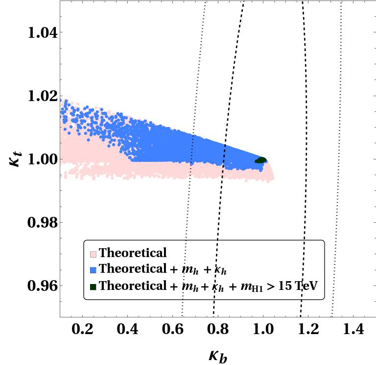
In this subsection, we discuss the interplay of various constraints from the Higgs data on the allowed values of parameters. All the parameters of the model, including pp and qq, are varied in the ranges described previously in sec. V.1 and in sec. V.3. We have calculated the values of κb\kappa_{b} and κt\kappa_{t} for each of these points and plotted them in fig. 5 in the κb−κt\kappa_{b}-\kappa_{t} plane.

The left panel of fig. 5 is for the simple basis and the right panel is for the generic basis. The pink points satisfy the theoretical constraints. We note that all pink points satisfy the experimental constraint on κt\kappa_{t} but only a fraction of them satisfy the constraint on κb\kappa_{b}. The points which satisfy the constraints on mhm_{h}, κW\kappa_{W}, κZ\kappa_{Z}, and κh\kappa_{h} form a small subset of pink points and are highlighted as blue points. We see that the κb\kappa_{b} constraint disallows about 9%9\% blue points. Finally, we impose the constraint on heavy Higgs mass mH1>15m_{H_{1}}>15 TeV. The points which satisfy this last constraint are shown in dark green. These green points essentially form a very small fraction (2.5%2.5\% of pink points) which are clustered around the point κb=1\kappa_{b}=1 and κt=1\kappa_{t}=1. This clustering around SM values of κb\kappa_{b} and κt\kappa_{t} is analogous to the scenario of ‘alignment by decoupling’ in two-Higgs-doublet model (2HDM) Gunion:2002zf. The Higgs sector of DLRSM effectively reduces to a special version of three-Higgs-doublet model at the electroweak scale, leading to this similarity with 2HDM.
Refer to caption
Refer to caption
Figure 5: Predictions for κb\kappa_{b} and κt\kappa_{t} for (a) simple and (b) generic basis with random values of quartic couplings in the ranges given by eqs. (36) and  (39) respectively. Additionally, pp and qq are varied logarithmically in the range [0.1,10][0.1,10]. The pink points satisfy the theoretical constraints, the blue points satisfy the additional mhm_{h} and κh\kappa_{h} constraints, and dark green points also satisfy constraint on heavy Higgs mass mH​1>15m_{H1}>15 TeV.

VI Summary and Outlook

We revisit the doublet left-right symmetric model with the scalar sector consisting of a bidoublet and two doublets. The two neutral scalars embedded in the bidoublet and the one from the S​U​(2)LSU(2)_{L} doublet can all contribute to EWSB. The pattern of the EWSB in this model is parametrized by the two ratios of vevs r=κ2/κ1r=\kappa_{2}/\kappa_{1} and w=vL/κ1w=v_{L}/\kappa_{1}. Most studies of DLRSM take these two ratios to be very small. In this paper, we study how the Higgs data from LHC constrains these two parameters. In particular, we check the consistency of the usual assumption r,w≪1r,w\ll 1 with the data.

In our study, we demand that the parameters of our model should be such that

  1. 1.

    the Higgs potential is bounded from below,

  2. 2.

    the quartic couplings of the Higgs potential should satisfy perturbative unitarity,

  3. 3.

    the Yukawa couplings, particularly of third of generation of fermions, should be perturbative,

  4. 4.

    the mass-squared values of all CP-even Higgses should be positive.

The third condition in the above list leads to upper limits r<0.8r<0.8 and w<3.5w<3.5, whereas the fourth condition requires the two ratios of quartic couplings,

p=(α3−α4)α4​and​q=(ρ2−2​ρ1)2​ρ1,p=\frac{(\alpha_{3}-\alpha_{4})}{\alpha_{4}}\,\,{\rm and}\,\,q=\frac{(\rho_{2}-2\rho_{1})}{2\rho_{1}},

to be positive. We vary the parameters of the model, subject to the above constraints and study which values of parameters satisfy the experimental constraints on the lightest CP-even scalar mass mhm_{h} and its coupling to gauge bosons κW\kappa_{W} and κZ\kappa_{Z}, its self-coupling κh\kappa_{h}, and its coupling to third generation quarks, κt\kappa_{t} and κb\kappa_{b}. We also imposed the additional constraint mH1>15m_{H_{1}}>15 TeV.

The model contains ten quartic couplings. In order to get a better understanding of the interplay of different quartic couplings, we defined a simplified set of quartic couplings: the three quartic couplings λi\lambda_{i}, involving only the bidoublet Higgs Φ\Phi, are set equal λ0\lambda_{0} and three of the quartic couplings αi\alpha_{i}, which couple the bidoublet to ordinary doublets χL\chi_{L} and χR\chi_{R}, are also set to equal to α0\alpha_{0}. A fourth λ\lambda coupling is defined in terms of the ratio x=λ2/λ4x=\lambda_{2}/\lambda_{4}, which is constrained to be in the range 0.25≤x≤0.850.25\leq x\leq 0.85 as shown in sec. IV. This simple set contains only six independent parameters, {λ0,α0,ρ1,x,p,q}\{\lambda_{0},\alpha_{0},\rho_{1},x,p,q\}.

We did our calculations first with the simple set of quartic couplings. We first fixed the value of the quartic coupling ratio q=1q=1 and considered four different values for the other quartic coupling ratio p=0.02,0.1,1,5p=0.02,0.1,1,5. For these values of pp and qq, we picked a random set of values for the other parameters in their allowed ranges. For each random set, we computed mh,κW,κZ,κh,κt,κbm_{h},\kappa_{W},\kappa_{Z},\kappa_{h},\kappa_{t},\kappa_{b} and mH1m_{H_{1}} and picked the points which satisfied the constraints on all the above quantities. We found that the points which satisfy the mhm_{h} constraint, typically satisfied the constraints from κW,κZ\kappa_{W},\kappa_{Z}, and κt\kappa_{t} also. The κh\kappa_{h} constraint rules out a significant number of points allowed by mhm_{h} for large values of ww. The constraint from κb\kappa_{b} has a non-trivial effect on the allowed points but the mH1>15m_{H_{1}}>15 TeV constraint rules out most of the points with low values of ww. For values of p≤0.1p\leq 0.1, there were no allowed points for w≲0.6w\lesssim 0.6. For p>1p>1, a few random points satisfy all the experimental constraints and have r<10−2r<10^{-2} and w<10−3w<10^{-3}. The number of such points, with very small values of rr and ww, steadily increase with increasing value of pp and form 14%14\% of all the allowed random points when p=5p=5. We find that such points also require ρ1>1\rho_{1}>1. Hence, we can conclude that the usual assumption that vL,κ2≪κ1v_{L},\kappa_{2}\ll\kappa_{1} holds true for only a fine-tuned set of parameters, in particular for somewhat large values of the quartic couplings ρ1\rho_{1} and ρ2\rho_{2}. This statement is true even when the value of qq is moved away from 11.

We repeated the above calculations with the full, generic set of quartic couplings. The low density of allowed points for small values of rr and ww not only persists in this case but becomes even more pronounced. Hence, our main conclusion is the following: Most of the studies of the DLRSM assume κ1≈v\kappa_{1}\approx v, with other vevs being negligibly small. On the contrary, we have pointed out that large values of rr and ww are allowed by the Higgs data and preferred by the indirect bound on mH​1m_{H1}. We also note that all the points satisfying mH1>15m_{H_{1}}>15 TeV constraint, also satisfy κt,b∼1\kappa_{t,\,b}\sim 1 to a very good precision. This confirms that the lightest scalar in DLRSM achieves alignment with the SM-like Higgs through the decoupling of the heavier scalars.

Acknowledgements.
S.K. would like to thank Tuhin S. Roy for valuable discussions. J.M. acknowledges the support of the Department of Science and Technology (DST) of the Government of India through grant no. SR/WOS-A/PM-6/2019(G). S.K. and S.U.S. thank Ministry of Education, Government of India, for financial support through Institute of Eminence funding.

Appendix A Heavy Higgs and gauge boson masses

In this section we present the expressions for the masses of the heavy scalars, and the masses and mixing of neutral gauge bosons.

(a)(a) Masses of the heavier CP-even neutral Higgses are given by

mH1,H22=14​y​(a1∓b1),mH32=2​ρ1​vR2,\displaystyle m^{2}_{H_{1},H_{2}}=\frac{1}{4y}(a_{1}\mp b_{1}),\,\,\,\,\,m^{2}_{H_{3}}=2\rho_{1}v_{R}^{2}, (41)

Masses of the heavier CP-odd neutral Higgses, A10A^{0}_{1} and A20A^{0}_{2} and the heavier charged scalars are given by

mA10,A202=14​y​(a2∓b2),mH1±,H2±2=14​y​(a3∓b3)m^{2}_{A^{0}_{1},A^{0}_{2}}=\frac{1}{4y}(a_{2}\mp b_{2})\,\,,\,\,\,\,m^{2}_{H^{\pm}_{1},H^{\pm}_{2}}=\frac{1}{4y}(a_{3}\mp b_{3}) (42)

where

x=1+r2,y=1−r2,\displaystyle x=1+r^{2},y=1-r^{2},
a1=vR2​(x​α34+2​ρ12​(2​w2+y)),\displaystyle a_{1}=v_{R}^{2}\big(x\alpha_{34}+2\rho_{12}(2w^{2}+y)\big),
a2=vR2​(x​α34+2​y​ρ12+2​w2​ρ12)+κ12​(−4​x​y​λ23+w2​(x​α34+2​y​ρ12)),\displaystyle a_{2}=v_{R}^{2}\Big(x\alpha_{34}+2y\rho_{12}+2w^{2}\rho_{12}\Big)+\kappa_{1}^{2}\Big(-4xy\lambda_{23}+w^{2}(x\alpha_{34}+2y\rho_{12})\Big),
a3=vR2​(x​α34+2​y​ρ12−4​w2​ρ12)+κ12​(2​y2​α34+x​w2​(α34−2​ρ12)),\displaystyle a_{3}=v_{R}^{2}\Big(x\alpha_{34}+2y\rho_{12}-4w^{2}\rho_{12}\Big)+\kappa_{1}^{2}\Big(2y^{2}\alpha_{34}+xw^{2}(\alpha_{34}-2\rho_{12})\Big),
b1=vR2​[(x​α34+2​ρ12​r4+4​r2​w2−1x)2+16​ρ122​r2​w2​(x+w2)​y2x2]1/2,\displaystyle b_{1}=v_{R}^{2}\Bigg[\Big(x\alpha_{34}+2\rho_{12}\frac{r^{4}+4r^{2}w^{2}-1}{x}\Big)^{2}+16\rho_{12}^{2}r^{2}w^{2}\frac{(x+w^{2})y^{2}}{x^{2}}\Bigg]^{1/2},
b2=[vR4(x2α232+4(4r2w2−xy)α34ρ12+(xy2+16r2w2(w2−yr2))ρ122)\displaystyle b_{2}=\Bigg[v_{R}^{4}\Big(x^{2}\alpha_{23}^{2}+4(4r^{2}w^{2}-xy)\alpha_{34}\rho_{12}+(xy^{2}+16r^{2}w^{2}(w^{2}-yr^{2}))\rho_{12}^{2}\Big)
+κ14​(−4​x​y​λ23+w2​(x​α34−2​y​ρ12))2+2​κ12​vR2​(8​r2​w4​ρ12​(α34−y​ρ12)−4​x​y​λ23​(x​α34−2​y​ρ12)CLOSE\displaystyle+\kappa_{1}^{4}\Big(-4xy\lambda_{23}+w^{2}(x\alpha_{34}-2y\rho_{12})\Big)^{2}+2\kappa_{1}^{2}v_{R}^{2}\Big(8r^{2}w^{4}\rho_{12}(\alpha_{34}-y\rho_{12})-4xy\lambda_{23}(x\alpha_{34}-2y\rho_{12})
+w2(x2α342−4y(xα34+8r2λ23)ρ12+4y2ρ122))]1/2,\displaystyle+w^{2}(x^{2}\alpha_{34}^{2}-4y(x\alpha_{34}+8r^{2}\lambda_{23})\rho_{12}+4y^{2}\rho_{12}^{2})\Big)\Bigg]^{1/2},
b3=[w4κ14(xα34−2yρ12)2+2vR2w2κ12(α342(4r2−y2)+4(y2−2r2y+2r2w2)α34ρ12\displaystyle b_{3}=\Bigg[w^{4}\kappa_{1}^{4}(x\alpha_{34}-2y\rho_{12})^{2}+2v_{R}^{2}w^{2}\kappa_{1}^{2}\Big(\alpha_{34}^{2}(4r^{2}-y^{2})+4(y^{2}-2r^{2}y+2r^{2}w^{2})\alpha_{34}\rho_{12}
−4y(y2−r2y+2r2w2)ρ122)+vR4(x2α342+4(4r2w2−xy)α34ρ12+4(y2−4r2y+4r2w4)ρ122)]1/2,\displaystyle-4y(y^{2}-r^{2}y+2r^{2}w^{2})\rho_{12}^{2}\Big)+v_{R}^{4}\Big(x^{2}\alpha_{34}^{2}+4(4r^{2}w^{2}-xy)\alpha_{34}\rho_{12}+4(y^{2}-4r^{2}y+4r^{2}w^{4})\rho_{12}^{2}\Big)\Bigg]^{1/2}\,\,\,,

where α34\alpha_{34}, λ23\lambda_{23}, and ρ12\rho_{12} were previously defined. These expressions have been presented in the limit μ4=0\mu_{4}=0.

(b)(b) The massive neutral gauge bosons, Z1μZ^{\mu}_{1} and Z2μZ^{\mu}_{2}, and photon AμA^{\mu} is expressed in terms of the unphysical fields as

Aμ\displaystyle A_{\mu} =\displaystyle= g~gL​WL​μ3+g~gR​WR​μ3+g~gB​L​Bμ,\displaystyle\frac{\tilde{g}}{g_{L}}W^{3}_{L\mu}+\frac{\tilde{g}}{g_{R}}W^{3}_{R\mu}+\frac{\tilde{g}}{g_{BL}}B_{\mu},
Z1​μ\displaystyle Z_{1\mu} =\displaystyle= 1D1​(gL​(8​mZ12−2​gR2​vR2)(gR2​vR2−gL2​vL2)​WL​μ3+gR​(8​mZ22−2​(gL2+gR2)​κ+2−2​gR2​vR2)(gR2​vR2−gL2​vL2)​WR​μ3+2​gB​L​Bμ),\displaystyle\frac{1}{D_{1}}\Big(\frac{g_{L}(8m_{Z_{1}}^{2}-2g_{R}^{2}v_{R}^{2})}{(g_{R}^{2}v_{R}^{2}-g_{L}^{2}v_{L}^{2})}W^{3}_{L\mu}+\frac{g_{R}(8m_{Z_{2}}^{2}-2(g_{L}^{2}+g_{R}^{2})\kappa_{+}^{2}-2g_{R}^{2}v_{R}^{2})}{(g_{R}^{2}v_{R}^{2}-g_{L}^{2}v_{L}^{2})}W^{3}_{R\mu}+2g_{BL}B_{\mu}\Big),
Z2​μ\displaystyle Z_{2\mu} =\displaystyle= 1D2​(−gL​(8​mZ22−2​gR​vR2−2​gB​L2​(vL2+vR2))(gL2​vL2−gR2​vR2)​WL​μ3CLOSE\displaystyle\frac{1}{D_{2}}\Big(\frac{-g_{L}(8m_{Z_{2}}^{2}-2g_{R}v_{R}^{2}-2g_{BL}^{2}(v_{L}^{2}+v_{R}^{2}))}{(g_{L}^{2}v_{L}^{2}-g_{R}^{2}v_{R}^{2})}W^{3}_{L\mu} (44)
OPEN+gR​(8​mZ22−2​gL​vL2−2​gB​L2​(vL2+vR2)CLOSE(gL2​vL2−gR2​vR2)​WR​μ3+2​gB​L​Bμ),\displaystyle\,\,\,\,\,\,\,\,\,\,\,\,\,\,\,+\frac{g_{R}(8m_{Z_{2}}^{2}-2g_{L}v_{L}^{2}-2g_{BL}^{2}(v_{L}^{2}+v_{R}^{2})}{(g_{L}^{2}v_{L}^{2}-g_{R}^{2}v_{R}^{2})}W^{3}_{R\mu}+2g_{BL}B_{\mu}\Big)\,\,\,\,,

where,

1g~2\displaystyle\frac{1}{\tilde{g}^{2}} =\displaystyle= 1gL2+1gR2+1gB​L2,\displaystyle\frac{1}{g_{L}^{2}}+\frac{1}{g_{R}^{2}}+\frac{1}{g_{BL}^{2}}\,\,\,,
D1\displaystyle D_{1} =\displaystyle= [4​gB​L2+1(gL2​vL2−gR2​vR2)2​(8​mZ22​(gL2+gR2)−4​gL2​gR2​κ+2−2​gL4​v2−2​gR4​V2)]1/2,\displaystyle\Big[4g_{BL}^{2}+\frac{1}{(g_{L}^{2}v_{L}^{2}-g_{R}^{2}v_{R}^{2})^{2}}\Big(8m_{Z_{2}}^{2}(g_{L}^{2}+g_{R}^{2})-4g_{L}^{2}g_{R}^{2}\kappa_{+}^{2}-2g_{L}^{4}v^{2}-2g_{R}^{4}V^{2}\Big)\Big]^{1/2}\,\,\,,
D2\displaystyle D_{2} =\displaystyle= [4​gB​L2+1(gL2​vL2−gR2​vR2)2​((gL2+gR2)​(8​mZ22−2​gB​L2​(vL2+vR2))−2​gL2​gR2​(vL2+vR2))]1/2.\displaystyle\Big[4g_{BL}^{2}+\frac{1}{(g_{L}^{2}v_{L}^{2}-g_{R}^{2}v_{R}^{2})^{2}}\Big((g_{L}^{2}+g_{R}^{2})(8m_{Z_{2}}^{2}-2g_{BL}^{2}(v_{L}^{2}+v_{R}^{2}))-2g_{L}^{2}g_{R}^{2}(v_{L}^{2}+v_{R}^{2})\Big)\Big]^{1/2}\,\,.

Appendix B Conditions for boundedness from below

In the presence of the most general doublet-bidoublet mixing, here we calculate the conditions for boundedness from below following the gauge orbit formulation of ref. Chauhan:2019fji; Bonilla:2015eha. The unique form of the quartic term multiplied by α2\alpha_{2} prohibits any simple modification of existing bounds. The quartic potential of our interest is given by eq. (3). We choose the following parametrization:

Tr​(Φ†​Φ)+(χL†​χL)+(χR†​χR)≡R2\text{Tr}(\Phi^{\dagger}\Phi)+(\chi_{L}^{\dagger}\chi_{L})+(\chi_{R}^{\dagger}\chi_{R})\equiv R^{2}

Tr​(Φ~†​Φ~)=Tr​(Φ†​Φ)≡R2​cos2⁡θ\text{Tr}(\tilde{\Phi}^{\dagger}\tilde{\Phi})=\text{Tr}(\Phi^{\dagger}\Phi)\equiv R^{2}\cos^{2}\theta

(χL†​χL)≡R2​sin2⁡θ​sin2⁡γ(\chi_{L}^{\dagger}\chi_{L})\equiv R^{2}\sin^{2}\theta\sin^{2}\gamma

(χR†​χR)≡R2​sin2⁡θ​cos2⁡γ(\chi_{R}^{\dagger}\chi_{R})\equiv R^{2}\sin^{2}\theta\cos^{2}\gamma

Tr​(Φ~†​Φ)/Tr​(Φ†​Φ)≡β​e−i​ω\text{Tr}(\tilde{\Phi}^{\dagger}\Phi)/\text{Tr}(\Phi^{\dagger}\Phi)\equiv\beta e^{-i\omega}

Tr​(Φ†​Φ~)/Tr​(Φ†​Φ)≡β​ei​ω\text{Tr}(\Phi^{\dagger}\tilde{\Phi})/\text{Tr}(\Phi^{\dagger}\Phi)\equiv\beta e^{i\omega}

(χL†​Φ​Φ†​χL)/Tr​(Φ†​Φ)​(χL†​χL)≡η1(\chi_{L}^{\dagger}\Phi\Phi^{\dagger}\chi_{L})/\text{Tr}(\Phi^{\dagger}\Phi)(\chi_{L}^{\dagger}\chi_{L})\equiv\eta_{1}

(χR†​Φ†​Φ​χR)/Tr​(Φ†​Φ)​(χR†​χR)≡η2(\chi_{R}^{\dagger}\Phi^{\dagger}\Phi\chi_{R})/\text{Tr}(\Phi^{\dagger}\Phi)(\chi_{R}^{\dagger}\chi_{R})\equiv\eta_{2}

(χL†​Φ~​Φ~†​χL)/Tr​(Φ~†​Φ~)​(χL†​χL)=η3(\chi_{L}^{\dagger}\tilde{\Phi}\tilde{\Phi}^{\dagger}\chi_{L})/\text{Tr}(\tilde{\Phi}^{\dagger}\tilde{\Phi})(\chi_{L}^{\dagger}\chi_{L})=\eta_{3}

(χR†​Φ~†​Φ~​χR)/Tr​(Φ~†​Φ~)​(χR†​χR)=η4,(\chi_{R}^{\dagger}\tilde{\Phi}^{\dagger}\tilde{\Phi}\chi_{R})/\text{Tr}(\tilde{\Phi}^{\dagger}\tilde{\Phi})(\chi_{R}^{\dagger}\chi_{R})=\eta_{4}\,,

where R>0R>0, {θ,γ}∈[0,π2]\{\theta,\gamma\}\in[0,\frac{\pi}{2}], β∈[0,1]\beta\in[0,1], and ω∈[0,2​π]\omega\in[0,2\pi]. The allowed range for these parameters is 12​(1−1−β2)<η1,2,3,4<12​(1+1−β2)\frac{1}{2}(1-\sqrt{1-\beta^{2}})<\eta_{1,2,3,4}<\frac{1}{2}(1+\sqrt{1-\beta^{2}}) along with

η1+η3=1,η2+η4=1.\displaystyle\eta_{1}+\eta_{3}=1,\,\,\,\,\,\eta_{2}+\eta_{4}=1. (46)

Using the parametric forms defined above we obtain

V4=R4​[cos4⁡θ​f1​(λi,β,ω)+sin4⁡θ​f2​(ρi,γ)+sin2⁡θ​cos2⁡θ​f3​(αi,γ,ηi)],V_{4}=R^{4}\left[\cos^{4}\theta\,f_{1}(\lambda_{i},\beta,\omega)+\sin^{4}\theta\,f_{2}(\rho_{i},\gamma)+\sin^{2}\theta\cos^{2}\theta\,f_{3}(\alpha_{i},\gamma,\eta_{i})\right]\,\,\,, (47)

where

f1​(λi,β,ω)≡14​(λ1+λ2​β2​cos⁡2​ω+λ3​β2+λ4​β​cos⁡ω),\displaystyle f_{1}(\lambda_{i},\beta,\omega)\equiv\frac{1}{4}(\lambda_{1}+\lambda_{2}\beta^{2}\cos{2\omega}+\lambda_{3}\beta^{2}+\lambda_{4}\beta\cos{\omega}),
f2​(ρi,γ)≡ρ1​sin4⁡γ+ρ1​cos4⁡γ+ρ2​sin2⁡γ​cos2⁡γ,\displaystyle f_{2}(\rho_{i},\gamma)\equiv\rho_{1}\sin^{4}\gamma+\rho_{1}\cos^{4}\gamma+\rho_{2}\sin^{2}\gamma\cos^{2}\gamma,
f3​(αi,γ,ηi)≡α1+2​α2​β​cos⁡ω+α3​(η1​sin2⁡γ+η2​cos2⁡γ)+α4​(η3​sin2⁡γ+η4​cos2⁡γ).\displaystyle f_{3}(\alpha_{i},\gamma,\eta_{i})\equiv\alpha_{1}+2\alpha_{2}\beta\cos{\omega}+\alpha_{3}(\eta_{1}\sin^{2}\gamma+\eta_{2}\cos^{2}\gamma)+\alpha_{4}(\eta_{3}\sin^{2}\gamma+\eta_{4}\cos^{2}\gamma).

Upon applying the copositivity criteria, eq. (47) indicates that

f1​(λi,β,ω)>0,\displaystyle f_{1}(\lambda_{i},\beta,\omega)>0, (48)
f2​(ρi,γ)>0,\displaystyle f_{2}(\rho_{i},\gamma)>0, (49)
f3​(αi,γ,ηi)+2​f1​(λi,β,ω)​f2​(ρi,γ)>0.\displaystyle f_{3}(\alpha_{i},\gamma,\eta_{i})+2\sqrt{f_{1}(\lambda_{i},\beta,\omega)f_{2}(\rho_{i},\gamma)}>0\,\,\,. (50)

These conditions should hold for all possible values of the parameters {β,ω,r,η1,2,3,4,γ}\{\beta,\omega,r,\eta_{1,2,3,4},\gamma\}.

∙\bullet f1​(λi,β,ω)f_{1}(\lambda_{i},\beta,\omega) is minimized at β=0\beta=0, or sin⁡ω=0\sin{\omega}=0, and cosω=−λ4/2λ2\cos\omega=-\lambda_{4}/2\lambda_{2}. Subsequently, certain combinations of λ\lambda s can be obtained Chauhan:2019fji

f1>0:{λ1(λ1−λ422​λ2+λ3)⟸2​λ2+λ3>|λ4|(λ1+λ3+2​(λ2−|λ4|))(λ1+λ3−2​λ2−λ424​λ2)⟸|4​λ2|>|λ4|}\displaystyle f_{1}>0:\left\{\begin{array}[]{lr}\lambda_{1}\\ \left(\lambda_{1}-\frac{\lambda_{4}^{2}}{2\lambda_{2}+\lambda_{3}}\right)\qquad\quad\>\impliedby 2\lambda_{2}+\lambda_{3}>|\lambda_{4}|\\ \left(\lambda_{1}+\lambda_{3}+2(\lambda_{2}-|\lambda_{4}|)\right)\\ \left(\lambda_{1}+\lambda_{3}-2\lambda_{2}-\frac{\lambda_{4}^{2}}{4\lambda_{2}}\right)\impliedby|4\lambda_{2}|>|\lambda_{4}|\\ \end{array}\right\}

Here the notation “p ⟸\impliedby q” implies condition p has to checked if and only if condition q is true.

∙\bullet f2​(ρi,γ)f_{2}(\rho_{i},\gamma) is symmetric under the exchange sin⁡γ↔cos⁡γ\sin\gamma\leftrightarrow\cos\gamma. Thus f2f_{2} becomes minimum at sin⁡γ=cos⁡γ=12\sin\gamma=\cos\gamma=\frac{1}{\sqrt{2}} and assumes the value f2,min≡2​ρ1+ρ24f_{2,\text{min}}\equiv\frac{2\rho_{1}+\rho_{2}}{4}. In the limits tan⁡γ=0\tan\gamma=0, and tan⁡γ=∞\tan\gamma=\infty, f2,min=ρ1f_{2,\text{min}}=\rho_{1}. This leads to the following boundedness criteria

f2>0:{ρ1>0,     2ρ1+ρ2>0}.\displaystyle f_{2}>0:\,\,\,\,\,\,\{\rho_{1}>0,\,\,\,\,\,2\rho_{1}+\rho_{2}>0\}\,\,\,\,. (56)

∙\bullet Eq. (50) is symmetric under the exchange η1↔η2,η3↔η4\eta_{1}\leftrightarrow\eta_{2},\eta_{3}\leftrightarrow\eta_{4}, along with sin⁡γ↔cos⁡γ\sin\gamma\leftrightarrow\cos\gamma. The LHS of eq. (50) thus takes a minimum value at η1=η2\eta_{1}=\eta_{2}, η3=η4\eta_{3}=\eta_{4} and sin⁡γ=cos⁡γ=12\sin\gamma=\cos\gamma=\frac{1}{\sqrt{2}},

α1+2​α2​β​cos⁡ω+α3​η1+α4​η3+2​f1​(λi,β,ω)​(2​ρ1+ρ24)>0\alpha_{1}+2\alpha_{2}\beta\cos{\omega}+\alpha_{3}\eta_{1}+\alpha_{4}\eta_{3}+2\sqrt{f_{1}(\lambda_{i},\beta,\omega)\left(\frac{2\rho_{1}+\rho_{2}}{4}\right)}>0 (57)

Eq. (46) implies that η1​(2)m​i​n=η3​(4)m​a​x\eta_{1(2)}^{min}=\eta_{3(4)}^{max} and vice versa. So third condition becomes

for​tan⁡γ=1:\displaystyle\text{for}\,\,\tan\gamma=1:
α1+2​α2​β​cos⁡ω+α32​(1±1−β2)+α42​(1∓1−β2)+f1​(λi,β,ω)​(2​ρ1+ρ24)>0,\displaystyle\alpha_{1}+2\alpha_{2}\beta\cos{\omega}+\frac{\alpha_{3}}{2}(1\pm\sqrt{1-\beta^{2}})+\frac{\alpha_{4}}{2}(1\mp\sqrt{1-\beta^{2}})+\sqrt{f_{1}(\lambda_{i},\beta,\omega)\left(\frac{2\rho_{1}+\rho_{2}}{4}\right)}>0,
(58)
for​tan⁡γ=0​or​tan⁡γ=∞:\displaystyle\text{for}\,\,\tan\gamma=0\,\,\text{or}\,\,\tan\gamma=\infty:
α1+2​α2​β​cos⁡ω+α32​(1±1−β2)+α42​(1∓1−β2)+f1​(λi,β,ω)​ρ1>0.\displaystyle\alpha_{1}+2\alpha_{2}\beta\cos{\omega}+\frac{\alpha_{3}}{2}(1\pm\sqrt{1-\beta^{2}})+\frac{\alpha_{4}}{2}(1\mp\sqrt{1-\beta^{2}})+\sqrt{f_{1}(\lambda_{i},\beta,\omega)\rho_{1}}>0\,\,.
(59)

The contribution from α2\alpha_{2} dependent term of V4V_{4} in eqs. (58) and (59) is given by f3~​(α2,β,ω)=2​α2​β​cos⁡ω\tilde{f_{3}}(\alpha_{2},\beta,\omega)=2\alpha_{2}\beta\cos{\omega} which has a minimum value at β=0\beta=0 or sin⁡ω=0\sin{\omega}=0.

Case 1: For β=0\beta=0, f3~​(α2,β,ω)=0\tilde{f_{3}}(\alpha_{2},\beta,\omega)=0.
Case 2: For sin⁡ω=0,cos⁡ω=±1\sin{\omega}=0,\,\,\cos{\omega}=\pm 1, which implies f3~​(α2,β,ω)=−2​|α2|​β\tilde{f_{3}}(\alpha_{2},\beta,\omega)=-2|\alpha_{2}|\beta
Case 3: On the boundary β=1\beta=1, f3~​(α2,β,ω)=−2​|α2|\tilde{f_{3}}(\alpha_{2},\beta,\omega)=-2|\alpha_{2}|.

Now we list the boundedness conditions emerging from eqs. (58) and (59) in the aforementioned limits.

  • •

    For β=0\beta=0,

    α1+α3+λ1​(2​ρ1+ρ2)>0\displaystyle\alpha_{1}+\alpha_{3}+\sqrt{\lambda_{1}(2\rho_{1}+\rho_{2})}>0
    α1+α4+λ1​(2​ρ1+ρ2)>0\displaystyle\alpha_{1}+\alpha_{4}+\sqrt{\lambda_{1}(2\rho_{1}+\rho_{2})}>0
    α1+α3+2​λ1​ρ1>0\displaystyle\alpha_{1}+\alpha_{3}+2\sqrt{\lambda_{1}\rho_{1}}>0
    α1+α4+2​λ1​ρ1>0.\displaystyle\alpha_{1}+\alpha_{4}+2\sqrt{\lambda_{1}\rho_{1}}>0\,\,\,. (60)
  • •

    For sin⁡ω=0\sin{\omega=0},

    α1−2​|α2|​|λ4|2​λ2+λ3+α32​(1±1−λ42(2​λ2+λ3)2)+α42​(1∓1−λ42(2​λ2+λ3)2)\displaystyle\alpha_{1}-2|\alpha_{2}|\frac{|\lambda_{4}|}{2\lambda_{2}+\lambda_{3}}+\frac{\alpha_{3}}{2}\left(1\pm\sqrt{1-\frac{\lambda_{4}^{2}}{(2\lambda_{2}+\lambda_{3})^{2}}}\right)+\frac{\alpha_{4}}{2}\left(1\mp\sqrt{1-\frac{\lambda_{4}^{2}}{(2\lambda_{2}+\lambda_{3})^{2}}}\right)
    +(λ1−λ422​λ2+λ3)​(2​ρ1+ρ2)>0,\displaystyle+\sqrt{\left(\lambda_{1}-\frac{\lambda_{4}^{2}}{2\lambda_{2}+\lambda_{3}}\right)(2\rho_{1}+\rho_{2})}>0\,\,\,,
    α1−2​|α2|​|λ4|2​λ2+λ3+α32​(1±1−λ42(2​λ2+λ3)2)+α42​(1∓1−λ42(2​λ2+λ3)2)\displaystyle\alpha_{1}-2|\alpha_{2}|\frac{|\lambda_{4}|}{2\lambda_{2}+\lambda_{3}}+\frac{\alpha_{3}}{2}\left(1\pm\sqrt{1-\frac{\lambda_{4}^{2}}{(2\lambda_{2}+\lambda_{3})^{2}}}\right)+\frac{\alpha_{4}}{2}\left(1\mp\sqrt{1-\frac{\lambda_{4}^{2}}{(2\lambda_{2}+\lambda_{3})^{2}}}\right)
    +(λ1−λ422​λ2+λ3)​ρ1>0.\displaystyle+\sqrt{\left(\lambda_{1}-\frac{\lambda_{4}^{2}}{2\lambda_{2}+\lambda_{3}}\right)\rho_{1}}>0\,\,\,. (61)
  • •

    For β=1\beta=1, sin⁡ω=0\sin{\omega}=0,

    α1−2​|α2|+α32+α42+(λ1+λ3+2​(λ2−|λ4|))​(2​ρ1+ρ2)>0,\displaystyle\alpha_{1}-2|\alpha_{2}|+\frac{\alpha_{3}}{2}+\frac{\alpha_{4}}{2}+\sqrt{\left(\lambda_{1}+\lambda_{3}+2(\lambda_{2}-|\lambda_{4}|)\right)(2\rho_{1}+\rho_{2})}>0\,\,,
    α1−2​|α2|+α32+α42+2​(λ1+λ3+2​(λ2−|λ4|))​ρ1>0.\displaystyle\alpha_{1}-2|\alpha_{2}|+\frac{\alpha_{3}}{2}+\frac{\alpha_{4}}{2}+2\sqrt{\left(\lambda_{1}+\lambda_{3}+2(\lambda_{2}-|\lambda_{4}|)\right)\rho_{1}}>0\,\,\,. (62)
  • •

    For β=1\beta=1, cosω=−λ4/2λ2\cos{\omega}=-\lambda_{4}/2\lambda_{2},

    α1−2​|α2|+α32+α42+(λ1+λ3−2​λ2−λ424​λ2)​(2​ρ1+ρ2)>0,\displaystyle\alpha_{1}-2|\alpha_{2}|+\frac{\alpha_{3}}{2}+\frac{\alpha_{4}}{2}+\sqrt{\left(\lambda_{1}+\lambda_{3}-2\lambda_{2}-\frac{\lambda_{4}^{2}}{4\lambda_{2}}\right)(2\rho_{1}+\rho_{2})}>0\,\,\,,
    α1−2​|α2|+α32+α42+2​(λ1+λ3−2​λ2−λ424​λ2)​ρ1>0.\displaystyle\alpha_{1}-2|\alpha_{2}|+\frac{\alpha_{3}}{2}+\frac{\alpha_{4}}{2}+2\sqrt{\left(\lambda_{1}+\lambda_{3}-2\lambda_{2}-\frac{\lambda_{4}^{2}}{4\lambda_{2}}\right)\rho_{1}}>0\,\,\,. (63)

Eqs. (B), (56), (60), (61), (62), and (63) together constitute the full set boundedness from below conditions in DLRSM.

References

  • (1) J. C. Pati and A. Salam, “Lepton Number as the Fourth Color,” Phys. Rev. D 10 (1974), 275-289 [erratum: Phys. Rev. D 11 (1975), 703-703].
  • (2) R. N. Mohapatra and J. C. Pati, “A Natural Left-Right Symmetry,” Phys. Rev. D 11 (1975), 2558.
  • (3) R. N. Mohapatra and J. C. Pati, “Left-Right Gauge Symmetry and an Isoconjugate Model of CP Violation,” Phys. Rev. D 11 (1975), 566-571.
  • (4) G. Senjanovic and R. N. Mohapatra, “Exact Left-Right Symmetry and Spontaneous Violation of Parity,” Phys. Rev. D 12 (1975), 1502.
  • (5) G. Senjanovic, “Spontaneous Breakdown of Parity in a Class of Gauge Theories,” Nucl. Phys. B 153 (1979), 334-364.
  • (6) K. S. Babu and V. S. Mathur, “Radiatively Induced Seesaw Mechanism for Neutrino Masses,” Phys. Rev. D 38 (1988), 3550.
  • (7) A. Zee, “A Theory of Lepton Number Violation, Neutrino Majorana Mass, and Oscillation,” Phys. Lett. B 93 (1980), 389 [erratum: Phys. Lett. B 95 (1980), 461].
  • (8) K. S. Babu and A. Thapa, “Left-Right Symmetric Model without Higgs Triplets,” [arXiv:2012.13420 [hep-ph]].
  • (9) P. Fileviez Perez and C. Murgui, “Lepton Flavour Violation in Left-Right Theory,” Phys. Rev. D 95 (2017) no.7, 075010 [arXiv:1701.06801 [hep-ph]].
  • (10) P. Fileviez Perez, C. Murgui and S. Ohmer, “Simple Left-Right Theory: Lepton Number Violation at the LHC,” Phys. Rev. D 94 (2016) no.5, 051701 [arXiv:1607.00246 [hep-ph]].
  • (11) V. Bernard, S. Descotes-Genon and L. Vale Silva, “Constraining the gauge and scalar sectors of the doublet left-right symmetric model,” JHEP 09 (2020), 088 [arXiv:2001.00886 [hep-ph]].
  • (12) V. Brdar and A. Y. Smirnov, “Low Scale Left-Right Symmetry and Naturally Small Neutrino Mass,” JHEP 02 (2019), 045 [arXiv:1809.09115 [hep-ph]].
  • (13) P. S. B. Dev, R. N. Mohapatra and Y. Zhang, “Probing the Higgs Sector of the Minimal Left-Right Symmetric Model at Future Hadron Colliders,” JHEP 05 (2016), 174 [arXiv:1602.05947 [hep-ph]].
  • (14) G. Aad et al. [ATLAS], “Search for a heavy charged boson in events with a charged lepton and missing transverse momentum from p​ppp collisions at s=13\sqrt{s}=13 TeV with the ATLAS detector,” Phys. Rev. D 100 (2019) no.5, 052013 [arXiv:1906.05609 [hep-ex]].
  • (15) G. Aad et al. [ATLAS], “Search for high-mass dilepton resonances using 139 fb-1 of p​ppp collision data collected at s=\sqrt{s}=13 TeV with the ATLAS detector,” Phys. Lett. B 796 (2019), 68-87 [arXiv:1903.06248 [hep-ex]].
  • (16) A. M. Sirunyan et al. [CMS], “Search for resonant and nonresonant new phenomena in high-mass dilepton final states at s\sqrt{s} = 13 TeV,” JHEP 07 (2021), 208 [arXiv:2103.02708 [hep-ex]].
  • (17) H. Georgi and S. Weinberg, “Neutral Currents in Expanded Gauge Theories,” Phys. Rev. D 17 (1978), 275.
  • (18) N. G. Deshpande, J. F. Gunion, B. Kayser and F. I. Olness, “Left-right symmetric electroweak models with triplet Higgs,” Phys. Rev. D 44 (1991), 837-858.
  • (19) P. A. Zyla et al. [Particle Data Group], “Review of Particle Physics,” PTEP 2020 (2020) no.8, 083C01.
  • (20) J. Chakrabortty, J. Gluza, T. Jelinski and T. Srivastava, “Theoretical constraints on masses of heavy particles in Left-Right Symmetric Models,” Phys. Lett. B 759 (2016), 361-368. [arXiv:1604.06987 [hep-ph]].
  • (21) J. Chakrabortty, P. Konar and T. Mondal, “Constraining a class of B−-L extended models from vacuum stability and perturbativity,” Phys. Rev. D 89 (2014) no.5, 056014 [arXiv:1308.1291 [hep-ph]].
  • (22) G. Chauhan, “Vacuum Stability and Symmetry Breaking in Left-Right Symmetric Model,” JHEP 12 (2019), 137 [arXiv:1907.07153 [hep-ph]].
  • (23) M. Frank, C. Majumdar, P. Poulose, S. Senapati and U. A. Yajnik, “Vacuum structure of Alternative Left-Right Model,” JHEP 03 (2022), 065 [arXiv:2111.08582 [hep-ph]].
  • (24) K. Kannike, “Vacuum stability conditions and potential minima for a matrix representation in lightcone orbit space,” Eur. Phys. J. C 81 (2021) no.10, 940 [arXiv:2109.01671 [hep-ph]].
  • (25) A. M. Sirunyan et al. [CMS], “A measurement of the Higgs boson mass in the diphoton decay channel,” Phys. Lett. B 805 (2020), 135425 [arXiv:2002.06398 [hep-ex]].
  • (26) [ATLAS], “A combination of measurements of Higgs boson production and decay using up to 139139 fb-1 of proton–proton collision data at s=\sqrt{s}= 13 TeV collected with the ATLAS experiment,” ATLAS-CONF-2020-027.
  • (27) [CMS], “Combined Higgs boson production and decay measurements with up to 137 fb-1 of proton-proton collision data at s\sqrt{s} = 13 TeV,” CMS-PAS-HIG-19-005.
  • (28) [ATLAS], “Constraints on the Higgs boson self-coupling from the combination of single-Higgs and double-Higgs production analyses performed with the ATLAS experiment,” ATLAS-CONF-2019-049.
  • (29) Y. Zhang, H. An, X. Ji and R. N. Mohapatra, “General CP Violation in Minimal Left-Right Symmetric Model and Constraints on the Right-Handed Scale,” Nucl. Phys. B 802 (2008), 247-279 [arXiv:0712.4218 [hep-ph]].
  • (30) J. F. Gunion and H. E. Haber, “The CP-conserving two Higgs doublet model: The Approach to the decoupling limit,” Phys. Rev. D 67 (2003), 075019 [arXiv:hep-ph/0207010 [hep-ph]].
  • (31) C. Bonilla, R. M. Fonseca and J. W. F. Valle, Phys. Rev. D 92 (2015) no.7, 075028 [arXiv:1508.02323 [hep-ph]].