Far-from-equilibrium universality in two-dimensional Heisenberg antiferromagnets
Abstract
We study the far-from-equilibrium dynamics of isolated two-dimensional Heisenberg antiferromagnets. We consider spin spiral initial conditions which imprint a position-dependent staggered-magnetization (or Neel order) in the two-dimensional lattice. Remarkably, we find a long-lived prethermal regime characterized by self-similar behavior of staggered magnetization fluctuations, although the system has no long-range order at finite energy and the staggered magnetization does not couple with conserved charges. Exploiting the separation of length scales introduced by the initial condition, we derive a simplified analytical model that allow us to compute the spatial-temporal scaling exponents and power-law distribution of the staggered magnetization fluctuations analytically, and find excellent agreement with numerical simulations using phase space methods. The scaling exponents are insensitive to details of the initial condition, in particular, no fine-tuning of energy is required to trigger the self-similar scaling regime. Compared with recent results on far-from-equilibrium universality on the Heisenberg ferromagnet, we find quantitatively distinct spatial-temporal scaling exponents, therefore suggesting that the same model with ferromagnetic and antiferromagnetic initial conditions can host different universal regimes. Our predictions are relevant to ultra-cold atoms simulators of Heisenberg magnets and driven antiferromagnetic insulators.
I Introduction
Many-body systems out of thermodynamic equilibrium can exhibit universal phenomena beyond conventional equilibrium paradigms. Prominent examples include turbulenceSreenivasan 1999; bookzakharov; Nazarenko 2011, ageingCalabrese and Gambassi 2005, coarseningBray 1994, surface growthKardar et al. 1986, breakdown of transportForster et al. 1977, and percolationTäuber 2014. One common theme in the study of equilibrium and out-of-equilibrium universality is the emergence of self-similar behavior: microscopically distinct models can be classified into universality classes sharing the same scaling exponents. Unlike systems at thermodynamic equilibrium, far-from-equilibrium systems break a symmetry associated to detailed-balanceSieberer et al. 2015; Crossley et al. 2017; Aron et al. 2018 and can therefore exhibit richer behaviors than their equilibrium counterparts with quantitatively distinct scaling exponents. Such rich behaviors have been observed in driven-dissipative systemsMitra et al. 2006; Dalla Torre et al. 2012; Sieberer et al. 2013; Marino and Diehl 2016; Chiocchetta et al. 2016a where an external drive pushes the system to a non-thermal steady state while dissipation maintains energy balance, and in quenches of isolated systems where the system acts as its own bathAarts and Berges 2002; Berges et al. 2004; Berges et al. 2008; Berges and Sexty 2011; Chandran et al. 2013; Berges et al. 2014; Berges et al. 2015; Maraga et al. 2015; Chiocchetta et al. 2016b; Berges 2015; Fujimoto and Tsubota 2016; Berges and Wallisch 2017; Schmied et al. 2019; Chiocchetta et al. 2017. These universal non-equilibrium regimes are now routinely probed in cold atom experimentsNavon et al. 2016; Eigen et al. 2018; Erne et al. 2018; Prüfer et al. 2018; Glidden et al. 2021.
Conserved charges and order parameters, both of which are determined by symmetries and dimensionality of the system, play an important role in determining the nature of the scaling behavior. In some cases, non-conventional scaling behavior arises from the non-linear dynamics of conserved charges in phase space. Examples include turbulent phenomena in fluids and non-thermal fixed points of bosonic theories where the self-similar scaling is governed by the cascade of conserved charges in momentum spacebookzakharov; Berges 2015; Fujimoto and Tsubota 2016; Berges and Wallisch 2017; Schmied et al. 2019, one-dimensional integrable systems where Kardar-Parisi-Zhang (KPZ) scaling arises due to the extensive number of conserved chargesBertini et al. 2015; Bulchandani et al. 2018; De Nardis et al. 2020; Gopalakrishnan and Vasseur 2019, and thermalizing systems in low dimensions which display a breakdown of local hydrodynamics Forster et al. 1977; Das et al. 2020; Delacrétaz and Glorioso 2020 (see Ref.Glorioso et al. 2022 for an example in kinematically constrained systems). In other cases, non-conventional scaling is induced by the dynamics of the order parameter. Examples include coarsening dynamics where self-similar scaling arises due to the growth of ordered domainsBray 1994; Rutenberg 1995; Rutenberg and Bray 1995, or ageing dynamics where self-similar scaling arises due to quasi-long range correlations close to criticalityGagel et al. 2014; Gagel et al. 2015; Sciolla and Biroli 2013; Chiocchetta et al. 2017. In general, quantities which are neither conserved nor couple with an order parameter are expected to relax in microscopic times and exhibit featureles fluctuations.
Here we study the prethermal dynamics of isolated Heisenberg antiferromagnets and show that quantities which are neither conserved nor exhibit ordering at finite temperature can still exhibit slow relaxation and universal prethermal dynamics when initialized from certain excited states. In particular, using spin spiral excited states with inhomogeneous Neel order (see Fig.1), we find that large and slowly-relaxing staggered magnetization fluctuations persist during a long-lived prethermal regime although the system exhibits no symmetry-breaking phase transition at finite temperature. In this prethermal regime, the staggered magnetization rapidly relaxes to zero but staggered magnetization fluctuations exhibit universal scaling given by:
| (1) |
with and . In Eq.(1), the universal function also exhibits scaling for a broad range of momenta, with . The scaling exponents () are universal in the sense that they are insensitive to details of the Hamiltonian or the initial condition. In particular, we emphasize that no fine-tuning of energy is needed. Using a continuous non-linear model describing long-wavelength spin modes combined with a kinetic theory of interacting quasiparticles at shorter wavelengths, we are able to derive analytically the three scaling exponents . These analytic values are shown to agree remarkably well with numerical simulations using phase space methods.
We find that the origin of the prethermal scaling is associated to the existence of spin modes whose gapless nature is protected by the global SU(2) symmetry. We show this by computing the unequal time spin-spin correlation functionBoguslavski and Piñeiro Orioli 2020, which exhibits linearly-dispersing gapless modes even though the prethermal state is far from the staggered ground state. A central insight in understanding the prethermal scaling in two-dimensional systems with SU(2) symmetry was discussed in recent works by one of us in the context of Heisenberg ferromagnetsBhattacharyya et al. 2020; Rodriguez-Nieva et al. 2022a. In the ferromagnetic case, the two-dimensional nature of the system bestows total magnetization fluctuations a long-range character. In addition, the combination of conserved magnetization and the constrained interactions resulting from the SU(2) symmetry gives rise to a universality class distinct from previously-studied instances of scaling. Similarly to the ferromagnetic case, the two-dimensional nature of the antiferromagnetic system can lead to quasi-long-range correlations of the staggered magnetization. However, unlike the ferromagnet, the staggered magnetization is not conserved. In spite of its non-conserved nature, we still find a parametrically long time window (controlled by non-universal parameters that depend on Hamiltonian details and the initial conditions) in which the system exhibits universal prethermal scaling.
As discussed in more detail below, we find that the Heisenberg antiferromagnet belongs to a different non-equilibrium universality class than previously-studied models with similar features. Compared to the Heisenberg ferromagnet, we find clearly distinct scaling exponents in spite of the underlying Hamiltonian being the same up to an overall sign. We attribute such differences to the different dispersion of emergent gapless modes and the different effective interactions between such modes, see Sec. III. We also emphasize that the scaling regime discussed in the present work is intrinsically different from the predictions of model G in the Halperin-Hohenberg classificationHohenberg and Halperin 1977: while the latter describes universal behaviour close to thermodynamic equilibrium, here we consider a dynamical regime where equilibrium properties, such as the fluctuation-dissipation relation, are violated. In comparison with theories in , we note that these also exhibit linearly-dispersing quasiparticles and long-range order at Sachdev 2011. We find that both theories and Heisenberg antiferromagnets exhibit similar (within numerical uncertainty) non-equilibrium spatial-temporal scaling exponents and while showing clearly distinct values of the universal scaling exponent . The same conclusion applies when comparing non-relativistic bosonic theories and antiferromagnets (we note that relativistic theories and non-relativistic theories were shown to exhibit the same and exponentsPiñeiro Orioli et al. 2015). We find that the difference in the exponent is related to the soft nature of the interaction between spin modes. We also note that the universal scaling in and theories is induced by gapped modes, whereas in antiferromagnets we observe gapless spin modes irrespective of the energy of the initial conditions.
Our predictions are relevant in a variety of experimental scenarios, both in condensed matter and cold atomic platforms. First, in recent years there has been remarkable advances in our experimental capabilities to probe the dynamics of isolated spin systems in low dimensionsHild et al. 2014; Jepsen et al. 2020; Jepsen et al. 2021. Current experiments are now able to prepare simple product states of excited spin spirals and tune the dimensionality and exchange interactions to probe the dynamics under different symmetries. Such experiments are now able to coherently evolve the system over unprecedentedly long timescales on the order of Jepsen et al. 2020 and, therefore, access the long-lived prethermal regime discussed in the present work. On a different front, experiments in solid-state systems are now able to drive low-dimensional ferromagnetic and antiferromagnetic insulators and probe magnetization fluctuations with energy resolution using local probesDu et al. 2017; Rodriguez-Nieva et al. 2022b; Zhou et al. 2021; Lee-Wong et al. 2021; Wang et al. 2021, such as nitrogen-vacancy centers in diamond. Such experiments are capable of directly measuring the power-law distribution in Eq.(1) as well as the relaxation dynamics of highly excited states.
The outline of the manuscript is as follows: In Sec. II, we describe the physical model and the intitial conditions. In Sec. III, we present a simple statistical mechanics model used to derive the scaling exponents analytically. In Sec. IV, we use phase space methods to numerically evaluate the scaling exponents. In Sec. V, we discuss the connections between our work and previously-studied instances of scaling in related models, and also present the conclusions. In the appendices we provide additional details about asymptotic functions used in Sec. III (Appendix A) and details about the statistical analysis used to analyze the numerical data (Appendix B).
II Microscopic model
We consider the Heisenberg antiferromagnet on a two-dimensional square lattice with nearest neighbour interactions:
| (2) |
Here are spin- operators, denotes summation over nearest neighbor spins and , and is a positive constant. For the purposes of our work, including additional next-nearest neighbour exchange does not affect the universal aspects of the dynamics, so long as the next-nearest-neighbor exchange does not induce frustration. As such, we restrict our discussion to nearest neighbour coupling only in order to keep the model as simple as possible. However, we emphasize that the SU(2) symmetry is essential to our discussion and breaking it will lead to qualitatively distinct results, as we discuss in more detail below.
For a large spin number and zero temperature, the Heisenberg antiferromagent exhibits a broken-symmetry ground state with a non-zero staggered magnetization (or Neel order). In this broken-symmetry state, the staggered magnetization has finite expectation value, with the lattice coordinate of spin (expressed in units of lattice constant, thus, are integer numbers). Unlike the ferromagnetic case (), the antiferromagnetic ground state is not classical and has zero point motion due to quantum fluctuations, i.e., . Interestingly, the broken-symmetry ground state is believed to be present even in the limitHuse and Elser 1988; Reger and Young 1988. For this reason, we expect that the universal aspects of dynamics discussed here will be independent of the spin number , although part of our analysis relies on the classical limit .
We consider an antiferromagnetic spin spiral product state as initial condition:
| (3) |
where . The initial condition (3) imprints a lengthscale in which spins have Neel order (although there is no order globally) while restricting dynamics in the zero magnetization sector . Dynamics of spin systems under this type of initial conditions are now routinely accessed in cold atomic platformsHild et al. 2014; Jepsen et al. 2020; Babadi et al. 2015; Rodriguez-Nieva et al. 2022c.
III Analytical derivation of the non-equilibrium scaling exponents
In this section, we proceed to construct a simplified non-equilibrium statistical mechanics model that captures the universal aspects of prethermalization in Heisenberg antiferromagnets, namely, the asymptotic form of the function and the numerical values of in Eq.(1). The essence of the approach follows closely that used in Refs.Rodriguez-Nieva 2021; Rodriguez-Nieva et al. 2022a and relies on exploiting the lengthscale separation of spin modes introduced by the initial condition, i.e., . The value of , which is time-dependent, defines a correlation length for staggered magnetization fluctuations. There are two types of excitations that need to be incorporated into our description. First, the initial excited state will trigger spatial fluctuations of Neel order which govern the dynamics of the staggered magnetization at wavevectors . Secondly, large-wavevector excitations will mediate the transfer of energy and magnetization towards UV degrees of freedom. Whereas the former is described with a classical continuum theory, the latter is described using kinetic theory for magnons within the wave turbulence formalism.
Following Ref.Rodriguez-Nieva 2021; Rodriguez-Nieva et al. 2022a we proceed in two steps. For wavevectors , we study the dynamics of magnetization fluctuations by assuming that the staggered magnetization is uniform in space: large wavevector magnons effectively see a uniform magnetization background within the collision timescale. As such, in Sec. III.1 we pin the antiferromagnetic order parameter and derive the effective kinetic theory for magnons. Using the wave turbulence formalism, we derive the power law exponent in Sec. III.2. In Sec. III.3, we study dynamics of the order parameter within a continuum theory and determine the relevant non-linearities that govern the resulting spatial-temporal scaling of magnetization fluctuations for wavevectors . From a simple scaling analysis that employs the equations of motion and spin conservation laws we derive the scaling exponents that govern the growth of .
III.1 Dynamics of short-wavelengths
In the presence of a uniform staggered magnetization, it is convenient to write the spin operators in terms of bosonic operators. Following Ref.Harris et al. 1971, we employ here the Dyson-Maleev transformation. Because of the antiferromagnetic nature of the ground state, we use two flavors of bosons to describe spins in the and sublattices (see Fig.1):
| (4a) | ||||
| (4b) | ||||
| (4c) | ||||
| (4d) | ||||
| (4e) | ||||
| (4f) | ||||
Here denotes , and are bosonic annihilation operators, and we use () to label sites in the () sublattice. We note that the Dyson-Maleev transformation produces the correct spin commutation relations but violates the property . In this case, the spin Hamiltonian becomes non-Hermitian. In contrast, the Holstein-Primakoff transformation—another commonly used transormation for spin systemsHolstein and Primakoff 1940—retains Hermiticity but generates an infinite series of interaction vertices. In spite of the non-hermiticity property, the Dyson-Maleev transformation has proven to be more convenient for studying spin-wave interaction in ferromagnets and antiferromagnets: it reproduces all the perturbative results obtained with the Holstein-Primakoff transformation in a much faster and compact wayHarris et al. 1971; Canali et al. 1992; Hamer et al. 1992.
Inserting Eqs.(4a)-(4f) into Eq. (2) and separating terms order by order, we find , with
| (5a) | ||||
| (5b) | ||||
Note that interactions are at small boson densities and vanish in the classical limit . Going into Fourier space and defining , , the quadratic component of the Hamiltonian is given by
| (6) |
Here denotes the phase factor , where denotes the nearest neighbor lattice vectors , and is the coordination number of each spin ( in a two-dimensional square lattice). The quartic component of the Hamiltonian is given by
with and .
We now proceed to diagonalize using the Bogoliubov transformation
| (7a) | |||
| (7b) | |||
where and are bosonic annihilation operators (bosonic commutation requires ). Replacing Eq.(7) into Eq.(6) leads to
| (8) |
and the factors and are given by
| (9) |
Using the Bogoliubov transformation on the quartic components of results in
| (10) |
where the phase factors are explicitly written in Appendix A.
We now analyze Eqs.(6) and (10) in the long wavelength limit in order to determine the power laws characterizing the quasiparticle dispersion and their interactions. From Eq.(6) one finds the well-known dispersion of small-momenta magnons given by . A second useful relation that results from the linearized analysis is the ratio between the amplitude of the staggered magnetization and the total magnetization. This relation can be obtained directly from the Bogoliubov eigenvectors in Eq.(9). Focusing on the staggered and total magnetization produced by the mode, we find that the staggered magnetization scales as , whereas the total magnetization scales as . Using the small wavevector expansion of Eq.(9), , and leads to , thus the total magnetization fluctuations are smaller that the staggered magnetization fluctuations and vanish in the limit, as expected for an antiferromagnet.
We now proceed to analyze the scaling of in Eq.(10) in the small wavevector limit. A detailed analysis of magnon relaxation in different energy ranges was done in Ref. Harris et al. 1971. Of primary interest in this work are on-shell processes describing particle-conserving collision between magnons with wavevectors . Off-resonant processes and processes which do not preserve particle number, both of which we will neglect, were shown to give subleading effects in the relaxation dynamics at small wavevectorsHarris et al. 1971. Thus, the relevant terms in Eq.(10) are those containing the phase factors , , and , with . For small wavevectors, the product scales as . In addition, the asymptotic form of is given by and the asymptotic form of is given by , see Appendix A, and they all scale as in the long wavelength limit. As such, the matrix element for the two-body interaction scales as .
As a side remark, we note that if SU(2) symmetry is broken, for example by adding anisotropic exchange, then the scaling with momentum of the interactions changes altogether. In particular, the phase factors become wavevector-independent and this would change the dynamical scaling laws characterizing the prethermal regime. In contrast, adding next-nearest neighbour exchange terms which preserve SU(2) symmetry will not alter the scaling behavior described in this work.
III.2 Scaling of the envelope function
We now calculate the power law scaling of the function using wave turbulence theory. Wave turbulence bookzakharov; Nazarenko 2011 provides a framework for computing the scaling of two-point correlation functions in far-from-equilibrium regimes when the system exhibits a weak coupling limit. In our case, the weak coupling limit is controlled by the parameter , see Eq.(5). The starting point in wave turbulence theory is to assume incoherent dynamics of the bosonic degrees of freedom and , i.e., , which is equivalent to assuming that transverse magnetization fluctuations (relative to the direction of the Neel order) are incoherent. This approximation is only valid when ; in the regime , instead, the Neel order will change its orientation, thus leading to finite expectation values for and (this regime will be analyzed in the next section). Under this approximation, each flavor of magnons is characterized by its occupation number and . The standard procedure in wave turbulence consists of: (i) deriving a kinetic equation from Eqs.(6) and (10) describing the time evolution of , (ii) proposing a solution of the form , and (iii) finding that gives rise to a steady-state solution (here we assume that ).
Following the discussion in the previous section, we employ an effective theory describing magnon excitations that only includes on-shell terms which preserve both particle number and energy. The exponent can only depend on the power of the quasiparticle dispersion , the power of the interaction, , and the system’s dimension . Based on the results of the previous section, we have and . As shown in Refs.bookzakharov; Nazarenko 2011, there are two non-thermal solutions with scaling exponents
| (11) |
The solution with scaling exponent is associated to a flux of quasiparticles cascading towards small momenta (inverse cascade), whereas the solution with scaling exponent is associated to a flux of energy cascading towards large momenta (direct cascade). The wavevector range where particle number is concentrated, , is where the quasiparticle cascade occurs, whereas the wavevector range where energy is concentrated, , is where the energy cascade occurs. Because , the inverse cascade characterizes scaling in the small wavevector regime whereas the energy cascade characterizes scaling at larger wavevectors. Using the values specific to our system, we find and .
Finally, we note that the scaling exponents and characterize the distribution of the occupation numbers and of the bosonic degrees of freedom rather than the spin degrees of freedom. Thus, the last step in our calculation is to transform back from bosonic operators into spin operators. We note that the spin operators are related to through a Bogoliubov transformation, see Eq.(7). As such, the scaling with momentum of the spin-spin correlation function is given by , thus .
We comment on the validity of the exponents and . In a strict sense, we need to question the validity of using a kinetic theory involving only on-resonant and particle conserving terms while neglecting all other processes. The validity of these approximations will be confirmed numerically in the next section. However, we emphasize that Ref. Harris et al. 1971 made a strong case to justify neglecting such processes for the smallest momenta magnons, which is the wavevector range described by the exponent . Instead, for larger-momenta magnons, which is the wavevector range described by the exponent , off-resonant processes and processes which do not preserve particle number become incrementally more relevant and the kinetic approximation begins to break down. Indeed, in our numerics below we find that the scaling exponent of matches remarkably well with but we do not observe a second wavevector range with exponent , which is consistent with the picture presented in Ref.Harris et al. 1971.
III.3 Spatio-temporal scaling exponents
In this section, we focus on the dynamics of magnetization fluctuations with wavevectors . We use the microscopic equations of motion in the continuum limit and analyze the role of leading order non-linearities to phenomenologically predict the exponents and governing the growth of . We define two spin fields and that characterize the average orientation of the spin in sublattice A and B, respectively. We also define the staggered magnetization and the total magnetization . Assuming that the fields and vary smoothly in space, we can expand the microscopic equations of motion for spins, to leading order in gradients:
| (12) | |||
| (13) |
where time is expressed in units of , and we approximated the sum over neighbouring spins with the laplacian, and . In terms of and , we find
| (14a) | ||||
| (14b) | ||||
To find the values of in Eq.(1), following Ref.Rodriguez-Nieva et al. 2022a we look at Eq.(14b) and balance the time derivative of with the leading nonlinearity, which is given by the first term on the right-hand-side:
| (15) |
with the Levi-Civita symbol. The second approximation that we use is that , which is justified from the linearized analysis of spin waves discussed above which showed that the total magnetization is smaller than the staggered magnetization. The final approximation that we use is to assume that all modes with wavevector are macroscopic and democratically occupied for all spin orientations. As such, if we identify in Eq.(1) and take at small wavevectors, then scales as and scales as . Using this scaling form in the left-hand-side of Eq.(15), we find , where we used . The right-hand side of Eq.(15), instead, yields , where we approximated and is the total area of the system. Equating both sides of Eq.(15) such that they both yield the same temporal scaling for results in
| (16) |
The second relation between and comes from the conservation of spin length, constant. Using the scaling and neglecting the contribution of the total magnetization , we find the second condition
| (17) |
Combining Eq.(16) with (17) in yields
| (18) |
We note that a similar analysis in the ferromagnetic case resulted in quantitatively different exponents and Rodriguez-Nieva et al. 2022a, indicating that the Heisenberg ferromagnet and antiferromagnet belong to different non-equilibrium universality classes. In particular, the same analysis leading to Eq.(16) resulted in the condition .
IV Numerical simulations through phase space methods
We compute the real time dynamics of quantum spins using the Truncated Wigner Approximation (TWA)Polkovnikov 2010; Davidson and Polkovnikov 2015; Schachenmayer et al. 2015; Zhu et al. 2019. This method incorporates quantum fluctuations by adding quantum noise in the initial conditions and evolving the classical trajectories using the classical equations of motion for spins . To sample the initial conditions in Eq.(3), we use a Gaussian approximation for the Wigner function given by
| (19) |
which reproduces the correct first and second moment of the Wigner distributionPolkovnikov 2010. In Eq.(19), we assumed without loss of generality that the initial spin is pointing in the direction.
Figure 2 shows the time evolution of the equal-time spin-spin correlation function for the staggered magnetization for a system of linear size , and initial conditions with wavevector , , and . At , only a single mode with wavevector is macroscopically occupied. Within a timescale on the order of the inverse energy (per spin), the macroscopic state is depleted and a power law distribution of the two-point correlation function develops. In this prethermal regime, we find that the values
| (20) |
best fit the numerical data in a sufficiently long time window, see details in Appendix B. These values agree with the analytical predictions of the previous section using scaling arguments.
We now proceed to analyze the power law scaling of the function in Eq.(1), see dashed lines in Fig.2(b). Interestingly, we observe only one power law characterizing the tails of the magnetization fluctuation distribution, contrary to the predictions of wave turbulence found in Sec. III.2 which suggested the existence of two exponents and . In fitting the power law exponent of the distribution we find that
| (21) |
which agrees with the exponent associated to the inverse particle cascade. This result is in agreement with the conclusions of Ref.Harris et al. 1971 which argues that off-resonant processes and particle-non-conserving can be neglected at small momenta, thus the effective theory (6)-(10) considering only particle conserving processes is a good approximation. For larger wavevectors (or energies), however, it is likely that off-resonant processes play a more prominent role and, therefore, the energy cascade exponent is not present.
We tested the robustness of our results using initial conditions with different values of , ranging from and different values of the wavevectors , and we consistently see the same scaling exponents within numerical uncertainty. Similarly to the Heisenberg ferromagnet, this suggests that the far-from-equilibrium dynamics of the isotropic Heisenberg antiferromagnet is governed by a single non-thermal fixed point with the exponents in (20) and (21). In contrast, U(1) theories were shown to exhibit multiple non-thermal fixed points, each of which can be activated by different initial conditions.
Whereas the groundstate of the Heisenberg antiferromagnet exhibits gapless low-energy excitations, it is unclear whether the highly excited initial condition in Eq.(3) leads to a dynamically-generated gap, such as those observed in and theories, or whether the spin modes in the self-similar region remain gapless. In a recent workRodriguez-Nieva et al. 2022a, it was shown that the global SU(2) symmetry of the Heisenberg ferromagnet precludes the opening of a dynamical gap during evolution, leading to a long-lived prethermal regime governed by gapless modes with dispersion . We numerically checked the nature of the excitations at the lowest wavevectors using the unequal-time correlation function for the staggered magnetization (), see Fig.2(c). Interestingly, we observe that the self-similar regime is governed by gapless modes at all times, even when the intermediate-time prethermal state is far from the ground state with uniform Neel order. The dispersion of the gapless mode is consistent with , different from the dispersion observed in the Heisenberg ferromagnet.

V Discussion and summary
The scaling regime discussed in the present work is intrinsically different from previously-studied instances of scaling in several important ways. Compared to the universal prethermal dynamics of Heisenberg ferromagnetsRodriguez-Nieva et al. 2022a, we find clearly distinct exponents originating from the existence of gapless modes with linear dispersion rather than modes with quadratic dispersion. In addition, unlike the ferromagnetic case, antiferromagnetic fluctuations are not coupled to any conserved charge. As such, the long-lived prethermal regime discussed here is cut off by some parametrically long timescale controlled by processes that give rise to staggered magnetization decay, see particle non-conserving terms in Eq. (10).
Heisenberg antiferromagnets and theories share many similarities at thermodynamic equilibrium and low temperatures, in particular, both exhibit linearly-dispersing quasiparticles and a symmetry-breaking phase transition at () in dimension (). We also find that they share some similarities in far-from-equilibrium regimes. For example, several works found the same scaling exponents and in theories regardless of the value of Piñeiro Orioli et al. 2015; Boguslavski and Piñeiro Orioli 2020. However, in theories quenched to (or across) a critical point Chandran et al. 2013; Maraga et al. 2015; Chiocchetta et al. 2017 self-similarity occurs only if parameters and initial conditions are fine-tuned so as to guarantee a vanishing late-time effective gap, unlike the antiferromagnetic case where we observe scaling without any fine-tuning of the initial conditions. In addition, we observe quantitative differences in the universal scaling function between both theories, reinforcing the idea that both models do not belong to the same non-equilibrium universality class.
Compared to non-thermal fixed points in bosonic theories, we note that models with symmetry in two dimensions can exhibit topological defects (vortices) which can qualitatively alter the far-from-equilibrium behavior and give rise to different self-similar scaling regimesNowak et al. 2011; Nowak et al. 2012. Even in the absence of vortices, the effective theory for the antiferromagnet (see Sec. III) differs from the bosonic theory both at the level of quasiparticle dispersion and their effective interactions, suggesting that both cannot belong to the same universality class. In certain cases, an effective gap has been observed to be dynamically generated by fluctuations Piñeiro Orioli et al. 2015; Boguslavski and Piñeiro Orioli 2020. This effective gap has been shown to lead to a modified non-relativistic effective theory at low momenta and share the same scaling exponents and characterizing theories and Heisenberg antiferromagnets. However, at the level of the universal scaling function in Eq.(1) we find a clearly distinct exponent which sets the dynamics of antiferromagnets and theories apart.
In summary, we studied the universal far-from-equilibrium dynamics of two-dimensional Heisenberg antiferromagnets. We showed that, if initialized in a state with inhomogeneous Neel order, magnetization fluctuations will exhibit a long-lived prethermal regime with universal behavior. This shows that quantities which are neither conserved nor exhibit long range order can still exhibit self-similiar behavior in a parametrically long time window. The scaling exponents are shown to be remarkably robust to details of the initial conditions—in particular, no fine-tuning of the energy is necessary. Our work also highlights the important role played by dimensionality and symmetry in giving rise to gapless spin modes with long range character. Combined with a recent work by one of us on Heisenberg ferromagnetsRodriguez-Nieva et al. 2022a, we have now fully characterized the non-thermal fixed points of the Heisenberg model both for ferromagnetic and antiferromagnetic exchange. The scaling regime discussed in this work is readily accessible in ongoing experiments in cold atomic gases which can probe these regimes in fully-tunable spin systemsJepsen et al. 2020; Duan et al. 2003; Davis et al. 2019, including tunable symmetries and spatial dimension.
Acknowledgements
We are grateful to Jamir Marino and Asier Piñeiro-Orioli for insightful comments and previous collaborations. JFRN acknowledges the Gordon and Betty Moore Foundation’s EPiQS Initiative through Grant GBMF4302 and GBMF8686, the 2021 KITP program Non-equilibrium universality: from classical to quantum and back, and the National Science Foundation under Grant No. NSF PHY-1748958. PG is supported by the Alfred P. Sloan Foundation through Grant FG-2020-13615, the Department of Energy through Award DE-SC0019380, and the Simons Foundation through Award No. 620869.
Appendix A Interaction coefficients within the Dyson-Maleev formalism
Here we reproduce the phase factor coefficients of the interactions in the Heisenberg Hamiltonian [Eq.(10)] within the Dyson-Maleev transformation [4a] using the notation in Ref.Harris et al. 1971. In particular, the phase factors appearing in the interactions of the effective Hamiltonian (10) are given by
| (22a) | ||||
| (22b) | ||||
| (22c) | ||||
| (22d) | ||||
| (22e) | ||||
In these expressions, the parameter is given by defined in the main text, where is the nearest neighbour lattice vectors in two-dimensions. The parameter is the ratio , with .
Of primary interest are the expressions in Eq.(22) in the long wavelength limit , particularly for the factors , and which contribute to particle-conserving scattering processes in the kinetic theory. We first note the following identities which hold in the asymptotic limit :
| (23a) | ||||
| (23b) | ||||
| (23c) | ||||
Replacing these asymptotic expressions into Eq.(22) and taking due to momentum conservation leads to
| (24a) | ||||
| (24b) | ||||
to leading order in momentum . These relations can also be written as:
| (25a) | ||||
Importantly, these phase factors accounting for particle-conserving processes scale as , which is used in the derivation of in Eq.(21) of the main text.
Appendix B Statistical analysis of numerical data
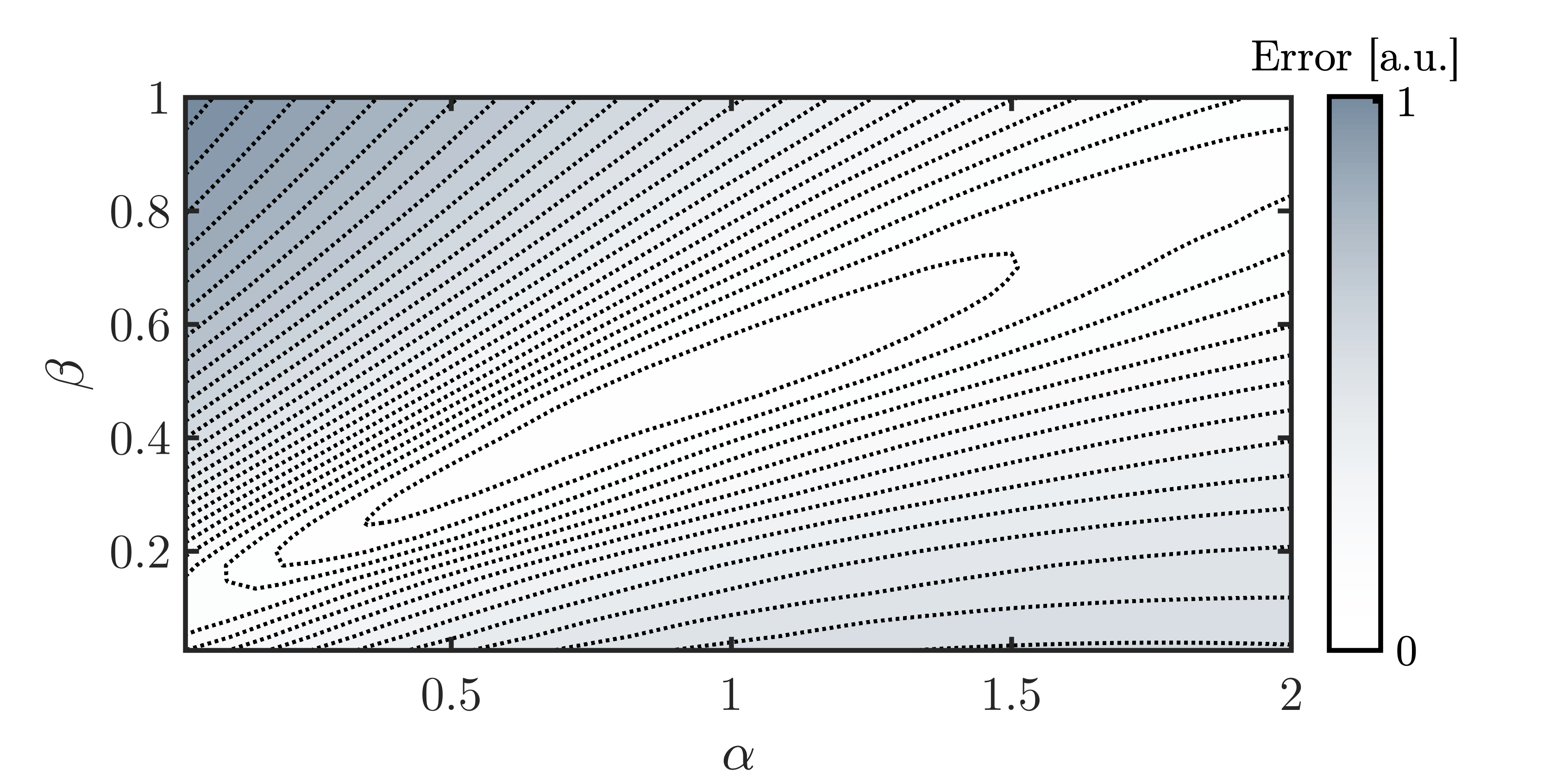
We obtain the scaling exponents and that best fit the numerical data by minimizing the error function that quantifies the collapse of the data points through the scaling in Eq.(1). First, we take discrete values of compatible with the inverse lattice spacing and evaluate the distribution at different time steps within the self-similar regime ( is roughly the inverse energy of the system). Second, we define the re-scaled variables and . By interpolating these variable, we are able to obtain an explicit function , where is assumed to be a continuum variable. Third, we compute the error function as
| (26) |
The contour plot of for the self-similar regime studied in Fig.2 is shown in Figure A1. We find that the best fitting with minimum error is centered around the point , which is consistent with our theoretical prediction. The error bars are obtained from the sensitivity of the parameter for different initial conditions.
References
- Sreenivasan (1999) Katepalli R. Sreenivasan, “Fluid turbulence,” Rev. Mod. Phys. 71, S383–S395 (1999).
- (2) V.E. Zakharov, V.S. L’vov, G. Falkovich, Kolmogorov Spectra of Turbulence I: Wave Turbulence, Springer Berlin Heidelberg (1992)
- Nazarenko (2011) S. Nazarenko, Wave Turbulence, Lecture Notes in Physics (Springer Berlin Heidelberg, 2011).
- Calabrese and Gambassi (2005) Pasquale Calabrese and Andrea Gambassi, “Ageing properties of critical systems,” Journal of Physics A: Mathematical and General 38, R133–R193 (2005).
- Bray (1994) A.J. Bray, “Theory of phase-ordering kinetics,” Advances in Physics 43, 357–459 (1994).
- Kardar et al. (1986) Mehran Kardar, Giorgio Parisi, and Yi-Cheng Zhang, “Dynamic scaling of growing interfaces,” Phys. Rev. Lett. 56, 889–892 (1986).
- Forster et al. (1977) Dieter Forster, David R Nelson, and Michael J Stephen, “Large-distance and long-time properties of a randomly stirred fluid,” Physical Review A 16, 732 (1977).
- Täuber (2014) Uwe C Täuber, Critical dynamics: a field theory approach to equilibrium and non-equilibrium scaling behavior (Cambridge University Press, 2014).
- Sieberer et al. (2015) LM Sieberer, A Chiocchetta, Andrea Gambassi, UC Täuber, and S Diehl, “Thermodynamic equilibrium as a symmetry of the Schwinger-Keldysh action,” Physical Review B 92, 134307 (2015).
- Crossley et al. (2017) Michael Crossley, Paolo Glorioso, and Hong Liu, “Effective field theory of dissipative fluids,” JHEP 09, 095 (2017).
- Aron et al. (2018) Camille Aron, Giulio Biroli, and Leticia F. Cugliandolo, “(Non) equilibrium dynamics: a (broken) symmetry of the Keldysh generating functional,” SciPost Phys. 4, 008 (2018).
- Mitra et al. (2006) Aditi Mitra, So Takei, Yong Baek Kim, and A. J. Millis, “Nonequilibrium quantum criticality in open electronic systems,” Phys. Rev. Lett. 97, 236808 (2006).
- Dalla Torre et al. (2012) Emanuele G Dalla Torre, Eugene Demler, Thierry Giamarchi, and Ehud Altman, “Dynamics and universality in noise-driven dissipative systems,” Physical Review B 85, 184302 (2012).
- Sieberer et al. (2013) LM Sieberer, Sebastian D Huber, E Altman, and S Diehl, “Dynamical critical phenomena in driven-dissipative systems,” Physical review letters 110, 195301 (2013).
- Marino and Diehl (2016) Jamir Marino and Sebastian Diehl, “Quantum dynamical field theory for nonequilibrium phase transitions in driven open systems,” Phys. Rev. B 94, 085150 (2016).
- Chiocchetta et al. (2016a) Alessio Chiocchetta, Andrea Gambassi, Sebastian Diehl, and Jamir Marino, “Universal short-time dynamics: Boundary functional renormalization group for a temperature quench,” Physical Review B 94, 174301 (2016a).
- Aarts and Berges (2002) Gert Aarts and Juergen Berges, “Classical aspects of quantum fields far from equilibrium,” Phys. Rev. Lett. 88, 041603 (2002).
- Berges et al. (2004) J. Berges, Sz. Borsányi, and C. Wetterich, “Prethermalization,” Phys. Rev. Lett. 93, 142002 (2004).
- Berges et al. (2008) Jürgen Berges, Alexander Rothkopf, and Jonas Schmidt, “Nonthermal fixed points: Effective weak coupling for strongly correlated systems far from equilibrium,” Phys. Rev. Lett. 101, 041603 (2008).
- Berges and Sexty (2011) Jürgen Berges and Dénes Sexty, “Strong versus weak wave-turbulence in relativistic field theory,” Phys. Rev. D 83, 085004 (2011).
- Chandran et al. (2013) Anushya Chandran, Arun Nanduri, Steven S Gubser, and Shivaji L Sondhi, “Equilibration and coarsening in the quantum model at infinite ,” Physical Review B 88, 024306 (2013).
- Berges et al. (2014) J. Berges, K. Boguslavski, S. Schlichting, and R. Venugopalan, “Turbulent thermalization process in heavy-ion collisions at ultrarelativistic energies,” Phys. Rev. D 89, 074011 (2014).
- Berges et al. (2015) J. Berges, K. Boguslavski, S. Schlichting, and R. Venugopalan, “Universality far from equilibrium: From superfluid Bose gases to heavy-ion collisions,” Phys. Rev. Lett. 114, 061601 (2015).
- Maraga et al. (2015) Anna Maraga, Alessio Chiocchetta, Aditi Mitra, and Andrea Gambassi, “Aging and coarsening in isolated quantum systems after a quench: Exact results for the quantum model with ,” Phys. Rev. E 92, 042151 (2015).
- Chiocchetta et al. (2016b) Alessio Chiocchetta, Marco Tavora, Andrea Gambassi, and Aditi Mitra, “Short-time universal scaling and light-cone dynamics after a quench in an isolated quantum system in spatial dimensions,” Phys. Rev. B 94, 134311 (2016b).
- Berges (2015) J. Berges, “Nonequilibrium Quantum Fields: From Cold Atoms to Cosmology,” arXiv e-prints , arXiv:1503.02907 (2015).
- Fujimoto and Tsubota (2016) Kazuya Fujimoto and Makoto Tsubota, “Direct and inverse cascades of spin-wave turbulence in spin-1 ferromagnetic spinor bose-einstein condensates,” Phys. Rev. A 93, 033620 (2016).
- Berges and Wallisch (2017) Jürgen Berges and Benjamin Wallisch, “Nonthermal Fixed Points in Quantum Field Theory Beyond the Weak-Coupling Limit,” Phys. Rev. D95, 036016 (2017).
- Schmied et al. (2019) Christian-Marcel Schmied, Aleksandr N. Mikheev, and Thomas Gasenzer, “Prescaling in a far-from-equilibrium bose gas,” Phys. Rev. Lett. 122, 170404 (2019).
- Chiocchetta et al. (2017) Alessio Chiocchetta, Andrea Gambassi, Sebastian Diehl, and Jamir Marino, “Dynamical crossovers in prethermal critical states,” Physical review letters 118, 135701 (2017).
- Navon et al. (2016) Nir Navon, Alexander L. Gaunt, Robert P. Smith, and Zoran Hadzibabic, “Emergence of a turbulent cascade in a quantum gas,” Nature 539, 72–75 (2016).
- Eigen et al. (2018) Christoph Eigen, Jake A. P. Glidden, Raphael Lopes, Eric A. Cornell, Robert P. Smith, and Zoran Hadzibabic, “Universal prethermal dynamics of bose gases quenched to unitarity,” Nature 563, 221–224 (2018).
- Erne et al. (2018) Sebastian Erne, Robert Bücker, Thomas Gasenzer, Jürgen Berges, and Jörg Schmiedmayer, “Universal dynamics in an isolated one-dimensional bose gas far from equilibrium,” Nature 563, 225–229 (2018).
- Prüfer et al. (2018) Maximilian Prüfer, Philipp Kunkel, Helmut Strobel, Stefan Lannig, Daniel Linnemann, Christian-Marcel Schmied, Jürgen Berges, Thomas Gasenzer, and Markus K. Oberthaler, “Observation of universal dynamics in a spinor bose gas far from equilibrium,” Nature 563, 217–220 (2018).
- Glidden et al. (2021) Jake A. P. Glidden, Christoph Eigen, Lena H. Dogra, Timon A. Hilker, Robert P. Smith, and Zoran Hadzibabic, “Bidirectional dynamic scaling in an isolated Bose gas far from equilibrium,” Nature Physics 17, 457–461 (2021).
- Bertini et al. (2015) Bruno Bertini, Fabian H. L. Essler, Stefan Groha, and Neil J. Robinson, “Prethermalization and thermalization in models with weak integrability breaking,” Phys. Rev. Lett. 115, 180601 (2015).
- Bulchandani et al. (2018) Vir B. Bulchandani, Romain Vasseur, Christoph Karrasch, and Joel E. Moore, “Bethe-Boltzmann hydrodynamics and spin transport in the XXZ chain,” Phys. Rev. B 97, 045407 (2018).
- De Nardis et al. (2020) Jacopo De Nardis, Sarang Gopalakrishnan, Enej Ilievski, and Romain Vasseur, “Superdiffusion from emergent classical solitons in quantum spin chains,” Physical Review Letters 125, 070601 (2020).
- Gopalakrishnan and Vasseur (2019) Sarang Gopalakrishnan and Romain Vasseur, “Kinetic theory of spin diffusion and superdiffusion in spin chains,” Phys. Rev. Lett. 122, 127202 (2019).
- Das et al. (2020) Avijit Das, Kedar Damle, Abhishek Dhar, David A Huse, Manas Kulkarni, Christian B Mendl, and Herbert Spohn, “Nonlinear fluctuating hydrodynamics for the classical xxz spin chain,” Journal of Statistical Physics 180, 238–262 (2020).
- Delacrétaz and Glorioso (2020) Luca V Delacrétaz and Paolo Glorioso, “Breakdown of diffusion on chiral edges,” Physical Review Letters 124, 236802 (2020).
- Glorioso et al. (2022) Paolo Glorioso, Jinkang Guo, Joaquin F. Rodriguez-Nieva, and Andrew Lucas, “Breakdown of hydrodynamics below four dimensions in a fracton fluid,” Nature Physics 18, 912 (2022).
- Rutenberg (1995) A. D. Rutenberg, “Scaling violations with textures in two-dimensional phase ordering,” Phys. Rev. E 51, R2715–R2718 (1995).
- Rutenberg and Bray (1995) A. D. Rutenberg and A. J. Bray, “Energy-scaling approach to phase-ordering growth laws,” Phys. Rev. E 51, 5499–5514 (1995).
- Gagel et al. (2014) Pia Gagel, Peter P Orth, and Jörg Schmalian, “Universal postquench prethermalization at a quantum critical point,” Physical review letters 113, 220401 (2014).
- Gagel et al. (2015) Pia Gagel, Peter P Orth, and Jörg Schmalian, “Universal postquench coarsening and aging at a quantum critical point,” Physical Review B 92, 115121 (2015).
- Sciolla and Biroli (2013) Bruno Sciolla and Giulio Biroli, “Quantum quenches, dynamical transitions, and off-equilibrium quantum criticality,” Physical Review B 88, 201110 (2013).
- Boguslavski and Piñeiro Orioli (2020) Kirill Boguslavski and Asier Piñeiro Orioli, “Unraveling the nature of universal dynamics in theories,” Phys. Rev. D 101, 091902 (2020).
- Bhattacharyya et al. (2020) Saraswat Bhattacharyya, Joaquin F. Rodriguez-Nieva, and Eugene Demler, “Universal prethermal dynamics in heisenberg ferromagnets,” Phys. Rev. Lett. 125, 230601 (2020).
- Rodriguez-Nieva et al. (2022a) Joaquin F. Rodriguez-Nieva, Asier Piñeiro Orioli, and Jamir Marino, “Far-from-equilibrium universality in the two-dimensional heisenberg model,” Proceedings of the National Academy of Sciences 119, e2122599119 (2022a).
- Hohenberg and Halperin (1977) P. C. Hohenberg and B. I. Halperin, “Theory of dynamic critical phenomena,” Rev. Mod. Phys. 49, 435–479 (1977).
- Sachdev (2011) Subir Sachdev, Quantum Phase Transitions, 2nd ed. (Cambridge University Press, 2011).
- Piñeiro Orioli et al. (2015) Asier Piñeiro Orioli, Kirill Boguslavski, and Jürgen Berges, “Universal self-similar dynamics of relativistic and nonrelativistic field theories near nonthermal fixed points,” Phys. Rev. D 92, 025041 (2015).
- Hild et al. (2014) Sebastian Hild, Takeshi Fukuhara, Peter Schauß, Johannes Zeiher, Michael Knap, Eugene Demler, Immanuel Bloch, and Christian Gross, “Far-from-equilibrium spin transport in heisenberg quantum magnets,” Phys. Rev. Lett. 113, 147205 (2014).
- Jepsen et al. (2020) Paul Niklas Jepsen, Jesse Amato-Grill, Ivana Dimitrova, Wen Wei Ho, Eugene Demler, and Wolfgang Ketterle, “Spin transport in a tunable heisenberg model realized with ultracold atoms,” Nature 588, 403–407 (2020).
- Jepsen et al. (2021) Paul Niklas Jepsen, Wen Wei Ho, Jesse Amato-Grill, Ivana Dimitrova, Eugene Demler, and Wolfgang Ketterle, “Transverse spin dynamics in the anisotropic heisenberg model realized with ultracold atoms,” arXiv preprint arXiv:2103.07866 (2021).
- Du et al. (2017) Chunhui Du, Toeno van der Sar, Tony X. Zhou, Pramey Upadhyaya, Francesco Casola, Huiliang Zhang, Mehmet C. Onbasli, Caroline A. Ross, Ronald L. Walsworth, Yaroslav Tserkovnyak, and Amir Yacoby, “Control and local measurement of the spin chemical potential in a magnetic insulator,” Science 357, 195–198 (2017).
- Rodriguez-Nieva et al. (2022b) Joaquin F. Rodriguez-Nieva, Daniel Podolsky, and Eugene Demler, “Probing hydrodynamic sound modes in magnon fluids using spin magnetometers,” Phys. Rev. B 105, 174412 (2022b).
- Zhou et al. (2021) Tony X. Zhou, Joris J. Carmiggelt, Lisa M. Gächter, Ilya Esterlis, Dries Sels, Rainer J. Stöhr, Chunhui Du, Daniel Fernandez, Joaquin F. Rodriguez-Nieva, Felix Büttner, Eugene Demler, and Amir Yacoby, “A magnon scattering platform,” Proceedings of the National Academy of Sciences 118, e2019473118 (2021).
- Lee-Wong et al. (2021) Eric Lee-Wong, Jinjun Ding, Xiaoche Wang, Chuanpu Liu, Nathan J. McLaughlin, Hailong Wang, Mingzhong Wu, and Chunhui Rita Du, “Quantum sensing of spin fluctuations of magnetic insulator films with perpendicular anisotropy,” Phys. Rev. Applied 15, 034031 (2021).
- Wang et al. (2021) Hailong Wang, Yuxuan Xiao, Mingda Guo, Eric Lee-Wong, Gerald Q. Yan, Ran Cheng, and Chunhui Rita Du, “Spin pumping of an easy-plane antiferromagnet enhanced by dzyaloshinskii–moriya interaction,” Phys. Rev. Lett. 127, 117202 (2021).
- Huse and Elser (1988) David A. Huse and Veit Elser, “Simple variational wave functions for two-dimensional heisenberg spin-1/2 antiferromagnets,” Phys. Rev. Lett. 60, 2531–2534 (1988).
- Reger and Young (1988) J. D. Reger and A. P. Young, “Monte carlo simulations of the spin-(1/2 heisenberg antiferromagnet on a square lattice,” Phys. Rev. B 37, 5978–5981 (1988).
- Babadi et al. (2015) Mehrtash Babadi, Eugene Demler, and Michael Knap, “Far-from-equilibrium field theory of many-body quantum spin systems: Prethermalization and relaxation of spin spiral states in three dimensions,” Phys. Rev. X 5, 041005 (2015).
- Rodriguez-Nieva et al. (2022c) Joaquin F. Rodriguez-Nieva, Alexander Schuckert, Dries Sels, Michael Knap, and Eugene Demler, “Transverse instability and universal decay of spin spiral order in the heisenberg model,” Phys. Rev. B 105, L060302 (2022c).
- Rodriguez-Nieva (2021) Joaquin F. Rodriguez-Nieva, “Turbulent relaxation after a quench in the heisenberg model,” Phys. Rev. B 104, L060302 (2021).
- Harris et al. (1971) A. B. Harris, D. Kumar, B. I. Halperin, and P. C. Hohenberg, “Dynamics of an antiferromagnet at low temperatures: Spin-wave damping and hydrodynamics,” Phys. Rev. B 3, 961–1024 (1971).
- Holstein and Primakoff (1940) T. Holstein and H. Primakoff, “Field dependence of the intrinsic domain magnetization of a ferromagnet,” Phys. Rev. 58, 1098–1113 (1940).
- Canali et al. (1992) C. M. Canali, S. M. Girvin, and Mats Wallin, “Spin-wave velocity renormalization in the two-dimensional heisenberg antiferromagnet at zero temperature,” Phys. Rev. B 45, 10131–10134 (1992).
- Hamer et al. (1992) C. J. Hamer, Zheng Weihong, and Peter Arndt, “Third-order spin-wave theory for the heisenberg antiferromagnet,” Phys. Rev. B 46, 6276–6292 (1992).
- Polkovnikov (2010) Anatoli Polkovnikov, “Phase space representation of quantum dynamics,” Annals of Physics 325, 1790–1852 (2010).
- Davidson and Polkovnikov (2015) Shainen M. Davidson and Anatoli Polkovnikov, “ semiclassical representation of quantum dynamics of interacting spins,” Phys. Rev. Lett. 114, 045701 (2015).
- Schachenmayer et al. (2015) J. Schachenmayer, A. Pikovski, and A. M. Rey, “Many-body quantum spin dynamics with monte carlo trajectories on a discrete phase space,” Phys. Rev. X 5, 011022 (2015).
- Zhu et al. (2019) Bihui Zhu, Ana Maria Rey, and Johannes Schachenmayer, “A generalized phase space approach for solving quantum spin dynamics,” arXiv e-prints , arXiv:1905.08782 (2019).
- Nowak et al. (2011) Boris Nowak, Dénes Sexty, and Thomas Gasenzer, “Superfluid turbulence: Nonthermal fixed point in an ultracold bose gas,” Phys. Rev. B 84, 020506 (2011).
- Nowak et al. (2012) Boris Nowak, Jan Schole, Dénes Sexty, and Thomas Gasenzer, “Nonthermal fixed points, vortex statistics, and superfluid turbulence in an ultracold bose gas,” Phys. Rev. A 85, 043627 (2012).
- Duan et al. (2003) L.-M. Duan, E. Demler, and M. D. Lukin, “Controlling spin exchange interactions of ultracold atoms in optical lattices,” Phys. Rev. Lett. 91, 090402 (2003).
- Davis et al. (2019) Emily J. Davis, Gregory Bentsen, Lukas Homeier, Tracy Li, and Monika H. Schleier-Smith, “Photon-mediated spin-exchange dynamics of spin-1 atoms,” Phys. Rev. Lett. 122, 010405 (2019).