An implicit FFT-based method for wave propagation in elastic heterogeneous media

The time interval $[0,T]$ is discretized in $N$ time increments of size $\Delta t=T/N$, such that

Eq. (2) has to be integrated in time, and the implicit Newmark integration scheme is used for this purpose. The velocity $\dot{u}$ and the acceleration $\ddot{u}$ of the time step $n$ are expressed as

where $\beta$ and $\gamma$ are two non-negative real numbers that define the version of the Newmark-$\beta$ method. The values $\beta=0.25$ and $\gamma=0.5$ are used to define the implicit unconditionally stable integration used.

Introducing the acceleration $\ddot{u}_{n}$ for a time $t_{n}$, from Eq. (5) in the conservation of linear momentum (Eq. (2)) leads to

where $f_{n}$ stands for the force density field prescribed at time $t_{n}$ and, for brevity, $u_{n}(x)$ has been written as $u_{n}$. Grouping the terms (unknown left, known right) and multiplying by the factor $-\beta\Delta t^{2}$ allows us to write the equation as

Equation (7) is a differential equation of the displacement at time $t_{n}$, and will be solved using Fourier transforms. To this aim, the derivatives therein have been computed using the definition of the derivatives in Fourier space of a scalar field $V(x)$:

On the right-hand side, let $\hat{b}_{n-1}$ be a term that groups the Fourier transform of all fields from the previous step,

Therefore, Eq. (9) can be condensed as;

The displacement field $\hat{u}_{n}$ in Fourier space is computed by solving two linear algebraic problems. The first provides $\hat{u}_{b}$,

and the second one provides the effect of a force $F$ on $x_{0}$, $\hat{u}_{f}$,

Note that the solution of this problem provides the Green’s function of the operator $\mathcal{A}(\cdot)$ for a force $F_{n}$ on the point $x_{0}$, $g(x,x_{0})$ which is defined as

In the case of a homogeneous medium, the linear operator $\mathcal{A}$ defines a Helmholtz equation with constant coefficients, and its Green’s function for an infinite medium has an analytical expression in real space, which is shown in appendix A. For a heterogeneous medium, the Green’s function $g(x,x_{0})$ can be obtained numerically and stored once at the beginning of the simulation by solving this linear problem.

The solution of the displacement can then be expressed as

which in real space corresponds to

Introducing in Eq. (17) the prescribed displacement at $x_{0}$, $u_{n}(x=x_{0})=U(t_{n})$ provides an equation to obtain the force $F_{n}$,

where $g^{-1}(x_{0},x_{0})$ is the inverse of the Green’s function on $x_{0}$, which represents the unit force to be applied at a point to produce a unit displacement. It is important to note that $g(x,x)$ is not singular at $x_{0}$, as it is shown in the appendix A.

Finally, once $F_{n}$ is determined by the previous equation , the displacement field $u_{n}(x)$ is obtained from Eq. (17).

In order to numerically solve the problem, the domain $\Omega$ will be divided into $N$ equal segments, and the values of the functions will be represented by their value in the center of each segment,

with $x_{m}=\frac{L}{N}(\frac{1}{2}+m)$ and $m\in[0,N-1]$. The point force defined using a delta function, $F_{n}=\int_{\Omega}f_{n}\delta(x-x_{0})\mathrm{d}\Omega$, is introduced in the discrete version as

The Fourier transform and its inverse will be approximated with the discrete Fourier transform that can be computed with the efficient FFT algorithm. The corresponding $N$ discrete frequencies in Fourier space are

The discrete version of the problem defined in Eqs. 10, 12 and 14 will be solved numerically using Krylov linear solvers. In particular, the linear equations will be solved in real space using the conjugate gradient. The resulting algorithm is given in Algorithm 1.

Solution for a homogeneous material: In the case of a homogeneous material, Young’s modulus and density are constant along the space material $E(x)=E$ and $\rho(x)=\rho$. In this case, $\hat{\mathcal{A}}^{-1}$ has a closed-form expression,

and there is no need to use CG to solve Eqs. (13) and (14).

Let $\Omega$ be a periodic prismatic domain in $d=2$ or $d=3$ dimensions, $\Omega=\left\{\mathbf{x}\ |\ 0\leq x_{i}\leq L_{i};1\leq i\leq d\right\}$, Fig. 2. The domain is occupied by a heterogeneous linear elastic medium, whose microstructure is characterized by the spatial distribution of the stiffness tensor and density $\mathbb{C}(\mathbf{x})$, $\rho(\mathbf{x})$, respectively.

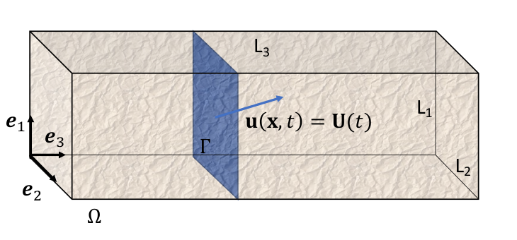
The problem consists in finding the periodic displacement field for a time interval $[0,T]$, $\mathbf{u}(\mathbf{x},t):\Omega\ \mathrm{x}\ [0,T]:\rightarrow\mathbb{R}^{d}$ such that the problem is in equilibrium, and the value of $\mathbf{u}(\mathbf{x},t)=\mathbf{U}(t)$ is prescribed in a lower-dimensional embedded manifold $\Gamma$ in $\mathbf{R}^{d}$, a curve if $d=2$ and a surface if $d=3$. To impose the displacement value at $\Gamma$, a force field $\mathbf{F}(\mathbf{x},t)$ that acts only on $\mathbf{x}\in\Gamma$ is introduced and its value is calculated at each time to satisfy the displacement condition on $\Gamma$. Note that since $\mathbf{u}$ is set as periodic, the macroscopic strain $\mathbf{E}=<\nabla^{s}\mathbf{u}>$ becomes equal to zero.

The starting point for solving the problem is the conservation of the linear momentum.

where $\mathbf{f}(\mathbf{x},t)$ is a force density field defined in $\Omega$, with dimensions of force per unit area or force per unit volume for $d=2$ and $d=3$, respectively. This force density field is zero everywhere but on the points lying on $\Gamma$ and can be expressed as

where $\delta_{\Gamma}(\mathbf{x})$ denotes the delta function extended to $\Gamma$ [44] and $\mathbf{F}(\mathbf{x},t)$ denotes a force density applied in $\Gamma$, with dimensions of force per unit length or force per unit volume, for $d$ = 2 and $d=3$, respectively. The properties of $\delta_{\Gamma}(\mathbf{x})$ are equivalent to the original Dirac delta,

The value of $\mathbf{F(x},t)$ along $\Gamma$ is obtained to satisfy the prescribed displacement on $\Gamma$

where $\mathbf{U}(t)$ is the time function defining the value of the displacement vector of all the points in $\Gamma$. The constitutive equation is the Hooke law for a general heterogeneous medium, characterized by the spatial distribution of its fourth-order stiffness tensor $\mathbb{C}(\mathbf{x})$,

As in the one-dimensional case, the Newmark integration scheme is applied to the linear momentum conservation (Eq. (22)) by substituting the acceleration definition given by Eq. (5). The linear momentum for time $t_{n}$ can then be written as a function of the displacement field $\mathbf{u}_{n}$ and the force density $\mathbf{f}_{n}$ in step $n$ (current step) and displacement $\mathbf{u}_{n-1}$, velocity $\dot{\mathbf{u}}_{n-1}$ and acceleration $\ddot{\mathbf{u}}_{n-1}$ in the previous step $n-1$.

As in the one-dimensional case, the left-hand side of Eq. (28) corresponds to a linear operator $\hat{\mathcal{A}}(\cdot)$ in Fourier space. Therefore, Eq. (28) can be written as

where $\widehat{\mathbf{f}}$ is the Fourier transform of the force density field at time $t=t_{n}$ (Eq. (23)) and $\hat{\mathcal{A}}\left(\hat{\mathbf{u}}\right)$ and $\hat{\mathbf{b}}$ are defined as (in components):

Due to the linearity of the operator $\hat{\mathcal{A}}\left(\hat{\mathbf{u}}\right)$, the problem can be split into two linear systems whose solutions will be added later. The first linear problem is

whose solution provides the field $\mathbf{u}_{b}=\mathcal{F}^{-1}\left\{\hat{\mathbf{u}}_{b}\right\}$. The second problem consists in finding the effect of the force density field $\mathbf{f}$, defined in Eq. (23), for a given value of the force $\mathbf{F}$ acting on $\Gamma$ at time $t=t_{n}$,

The solution $\mathbf{u}_{n}$ in real space corresponds to the sum of the solution of the two problems (Eqs. (32) and (33)),

At this stage, the value of the force density $\mathbf{F}$ acting at each point of $\Gamma$ is not yet known and should be obtained to meet the prescribed displacement. To obtain its value, Green’s functions will be used. Green’s function of the operator $\mathcal{A}$ provides the effect of a point force $\mathbf{P}$ concentrated on $\mathbf{x}^{\prime}$ on the displacement at a point $\mathbf{x}$,

The effect of a field $\mathbf{f}$ is then

where the convolution is performed at the points on $\Gamma$. The value of the force distributed on $\Gamma$ must be determined at each time step to satisfy the value of the prescribed displacement for the points in $\mathbf{x}\in\Gamma$,

and can be obtained inverting the previous equation,

where $\mathbf{g}^{-1}$ stands for the inverse of Green’s function. Solving Eq. (37) can be easily handled when the manifold $\Gamma$ is discretized. In this case, $\mathbf{g}(\mathbf{x,x}^{\prime})$ can be replaced by a matrix that links the forces and displacement of every point in $\Gamma$.This matrix is formed by solving Eq. (33) for each point in $\Gamma$ and its inverse, $\mathbf{g}^{-1}$, is calculated and only once and then is stored and used during the simulation. At each time step, $\mathbf{F}(\mathbf{x},t)$ is obtained using that inverse matrix. Finally, the force field $\mathbf{f}(\mathbf{x},t)=\delta_{\Gamma}\mathbf{F}(\mathbf{x},t)$ is used as the RHS of Eq. (33) to obtain $u_{f}$, and the displacement field is obtained using Eq. (34).

Focusing on the numerical resolution of the three-dimensional case, the periodic domain is discretized in $N_{1}\cdot N_{2}\cdot N_{3}$ equispaced voxels, whose centers are given by

with $(i,j,k)\in[0,N_{1}-1]\times[0,N_{2}-1]\times[0,N_{3}-1]$. The values of the properties of the material in each voxel $\mathbb{C}(\mathbf{x}_{i,j,k})$ and $\rho(\mathbf{x}_{i,j,k})$ correspond to the property of the material that occupies that position. The displacement vector is discretized using its value in the center of each voxel, $\mathbf{u}(\mathbf{x}_{i,j,k})$.

The discrete fields in Fourier space have the same dimension as their counterparts in real space. The corresponding $N_{1}\cdot N_{2}\cdot N_{3}$ discrete frequencies in Fourier space are

being the frequencies in each direction $\xi_{k_{1}},\xi_{k_{2}},\xi_{k_{3}}$ defined as in the 1D case, (Eq. 20).

After discretization, the linear operator $\hat{\mathcal{A}}$ defined in equation (30) is replaced by its discrete counterpart in which the Fourier and inverse Fourier transforms are substituted by discrete Fourier transforms, and the frequencies used are the discrete set defined in equation (39). The equations of the type $\hat{\mathcal{A}}(\mathbf{u})=\mathbf{b}$, as Eqs. ((32),(33)), correspond to a linear system of equations, which can be solved efficiently using Krylov iterative solvers. In the present case, the conjugate gradient can be used because of the Hermitian nature of the operator. Moreover, as proposed in [45] and [14] for similar problems, preconditioners can be built that strongly improve numerical performance. The proposed preconditioner is the exact solution of the linear equation for a homogeneous medium with average volume stiffness and density $\mathbb{C}=\overline{\mathbb{C}(\mathbf{x})}$ and $\rho=\overline{\rho(\mathbf{x})}$, and corresponds to

where $\mathbf{I}$ is the identity tensor and $\mathbf{K}(\bm{\xi})$ is the acoustic tensor, defined for each frequency as

The preconditioner, Eq.(40), is formed and stored once at the beginning of the simulation. Its computation is not expensive computationally since it only requires the inversion of a 3$\times$3 matrix for each frequency. This step is indeed equivalent to form the Gamma operator in a standard homogenization FFT simulation. The use of the preconditioner within the conjugate gradient implies just adding a multiplication of the current value of $\hat{\mathbf{u}}$ by $\hat{\mathcal{M}}$ at each iteration.

For obtaining the force distribution on $\Gamma$ at every time step, the Eq. (37) have to be solved. To perform this efficiently, the discrete inverse Green operator will be constructed once at the beginning of the simulation and used in subsequent time steps. Let $\mathbf{x}_{p}$ be the position of a point lying in $\Gamma$, $1\leq p\leq N_{p}$ and let $\mathbf{f}_{p}^{j}(\mathbf{x})$, be a force density field defined as

for every point $p$ and direction $j=1,2,3$. The displacement result of applying this field is obtained by solving the linear system,

where $\mathbf{u}_{(p,j)}(\mathbf{x})=\mathcal{F}^{-1}(\hat{\mathbf{u}}_{(p,j)})$. The result of solving the problem for each applied field around $p$ allows to form the Green’s tensor for each other point $q$ lying on $\Gamma$, $\mathbf{g}(q,p),p,q=1,N_{p}$, with dimensions $3\times 3$ which is defined as

The assembly of all $\mathbf{g}(p,q)$ matrices defines a new matrix, $\mathbf{G}$, with dimension $3N_{p}\times 3N_{p}$ as

which express the relation between displacement and the forces of the $N_{p}$ nodes in $\Gamma$. The convolution restricted to the manifold $\Gamma$ defined in Eq. (35) is therefore written, for the discrete case, as the matrix vector product in Eq. (46).

References

- [1] A. B. Bhatia. Scattering of high‐frequency sound waves in polycrystalline materials. The Journal of the Acoustical Society of America, 31(1):16–23, 1959.
- [2] Y. Tanaka, Y. Tomoyasu, and S.I. Tamura. Band structure of acoustic waves in phononic lattices: Two-dimensional composites with large acoustic mismatch. Physical Review B, 62(11):7387, 2000.
- [3] M. Jaafar, H. Mamtaz, M. H. Fouladi, M. Al-Atabi, and S. Narayana Namasivayam. Acoustic absorption of natural fiber composites. Journal of Engineering, 2016:5836107, 2016.
- [4] K. Attenborough. Acoustical characteristics of porous materials. Physics reports, 82(3):179–227, 1982.
- [5] N. A. Fleck, V. S. Deshpande, and M. F. Ashby. Micro-architectured materials: past, present and future. Proceedings of the Royal Society A: Mathematical, Physical and Engineering Sciences, 466(2121):2495–2516, 2010.
- [6] Y. Chen and S. Ghosh. Micromechanical analysis of strain rate-dependent deformation and failure in composite microstructures under dynamic loading conditions. International Journal of Plasticity, 32-33:218–247, 2012.
- [7] E. J. Lieberman, R. A. Lebensohn, D. B Menasche, C. A. Bronkhorst, and A. D. Rollett. Microstructural effects on damage evolution in shocked copper polycrystals. Acta Materialia, 116:270–280, 2016.
- [8] J.D. Clayton. Modeling dynamic plasticity and spall fracture in high density polycrystalline alloys. International Journal of Solids and Structures, 42(16):4613–4640, 2005.
- [9] G.W. Milton and A.T. Sawicki. Theory of Composites. Cambridge Monographs on Applied and Computational Mathematics. Applied Mechanics Reviews, 56(2):B27–B28, 03 2003.
- [10] J. Segurado, R. A. Lebensohn, and J. LLorca. Chapter one - computational homogenization of polycrystals. In Advances in Crystals and Elastic Metamaterials, volume 51 of Advances in Applied Mechanics, pages 1 – 114. Elsevier, 2018.
- [11] K. Matouš, M. G.D. Geers, V. G. Kouznetsova, and A. Gillman. A review of predictive nonlinear theories for multiscale modeling of heterogeneous materials. Journal of Computational Physics, 330:192–220, 2017.
- [12] M. S. Kushwaha, P. Halevi, L. Dobrzynski, and B. Djafari-Rouhani. Acoustic band structure of periodic elastic composites. Phys. Rev. Lett., 71:2022–2025, 1993.
- [13] H. I. Mahmoud. Reduced bloch mode expansion for periodic media band structure calculations. Proceedings of the Royal Society A, 465:2825–2848, 2009.
- [14] J. Segurado and R. A. Lebensohn. An fft-based approach for bloch wave analysis: application to polycrystals. Computational Mechanics, 68(5):981–1001, 2021.
- [15] A. Van Pamel, G. Sha, S. I. Rokhlin, and M. J. S. Lowe. Finite-element modelling of elastic wave propagation and scattering within heterogeneous media. Proceedings of the Royal Society A: Mathematical, Physical and Engineering Sciences, 473(2197):20160738, 2017.
- [16] M. Huang, G. Sha, P. Huthwaite, S. I. Rokhlin, and M. J. S. Lowe. Maximizing the accuracy of finite element simulation of elastic wave propagation in polycrystals. The Journal of the Acoustical Society of America, 148(4):1890–1910, 2020.
- [17] A. Sridhar, V.G. Kouznetsova, and M.G.D. Geers. A general multiscale framework for the emergent effective elastodynamics of metamaterials. Journal of the Mechanics and Physics of Solids, 111:414–433, 2018.
- [18] K. J. Bathe. Conserving energy and momentum in nonlinear dynamics: A simple implicit time integration scheme. Computers & Structures, 85(7):437–445, 2007.
- [19] G. Noh and K. J. Bathe. An explicit time integration scheme for the analysis of wave propagations. Computers & Structures, 129:178–193, 2013.
- [20] K. C. Park, S. J Lim, and H. Huh. A method for computation of discontinuous wave propagation in heterogeneous solids: basic algorithm description and application to one-dimensional problems. International Journal for Numerical Methods in Engineering, 91(6):622–643, 2012.
- [21] Elena Zampieri and Luca F. Pavarino. Isogeometric collocation discretizations for acoustic wave problems. Computer Methods in Applied Mechanics and Engineering, 385:114047, 2021.
- [22] M. Kronbichler, S. Schoeder, C. Müller, and W. A. Wall. Comparison of implicit and explicit hybridizable discontinuous galerkin methods for the acoustic wave equation. International Journal for Numerical Methods in Engineering, 106(9):712–739, 2016.
- [23] Junqi Zhang, Ankit Ankit, Hauke Gravenkamp, Sascha Eisenträger, and Chongmin Song. A massively parallel explicit solver for elasto-dynamic problems exploiting octree meshes. Computer Methods in Applied Mechanics and Engineering, 380:113811, 2021.
- [24] F. Auricchio, L. Beirão da Veiga, T.J.R. Hughes, A. Reali, and G. Sangalli. Isogeometric collocation for elastostatics and explicit dynamics. Computer Methods in Applied Mechanics and Engineering, 249-252:2–14, 2012. Higher Order Finite Element and Isogeometric Methods.
- [25] M. Stanglmeier, N.C. Nguyen, J. Peraire, and B. Cockburn. An explicit hybridizable discontinuous galerkin method for the acoustic wave equation. Computer Methods in Applied Mechanics and Engineering, 300:748–769, 2016.
- [26] Elena Zampieri and Luca F. Pavarino. Explicit second order isogeometric discretizations for acoustic wave problems. Computer Methods in Applied Mechanics and Engineering, 348:776–795, 2019.
- [27] S Lucarini, M V Upadhyay, and J Segurado. FFT based approaches in micromechanics: fundamentals, methods and applications. Modelling and Simulation in Materials Science and Engineering, 30(2):023002, 2021.
- [28] M. Schneider. A review of nonlinear fft-based computational homogenization methods. Acta Mechanica, 232(6):2051–2100, 2021.
- [29] H. Moulinec and P. Suquet. A fast numerical method for computing the linear and nonlinear mechanical properties of composites. Comptes Rendus de l’Académie des Sciences, 318:1417–1423, 1994.
- [30] S. Lucarini, L. Cobian, A. Voitus, and J. Segurado. Adaptation and validation of fft methods for homogenization of lattice based materials. Computer Methods in Applied Mechanics and Engineering, 388:114223, 2022.
- [31] T.W.J. de Geus, J. Vondřejc, J. Zeman, R.H.J. Peerlings, and M.G.D. Geers. Finite strain fft-based non-linear solvers made simple. Computer Methods in Applied Mechanics and Engineering, 318:412–430, 2017.
- [32] Yang Chen, Dmytro Vasiukov, Lionel Gélébart, and Chung Hae Park. A fft solver for variational phase-field modeling of brittle fracture. Computer Methods in Applied Mechanics and Engineering, 349:167–190, 2019.
- [33] Felix Ernesti, Matti Schneider, and Thomas Böhlke. Fast implicit solvers for phase-field fracture problems on heterogeneous microstructures. Computer Methods in Applied Mechanics and Engineering, 363:112793, 2020.
- [34] Noé Brice Nkoumbou Kaptchouang and Lionel Gélébart. Multiscale coupling of fft-based simulations with the ldc approach. Computer Methods in Applied Mechanics and Engineering, 394:114921, 2022.
- [35] Christian Gierden, Julian Kochmann, Johanna Waimann, Tobias Kinner-Becker, Jens Sölter, Bob Svendsen, and Stefanie Reese. Efficient two-scale fe-fft-based mechanical process simulation of elasto-viscoplastic polycrystals at finite strains. Computer Methods in Applied Mechanics and Engineering, 374:113566, 2021.
- [36] Elena Zampieri and A Tagliani. Numerical approximation of elastic waves equations by implicit spectral methods. Computer methods in applied mechanics and engineering, 144(1-2):33–50, 1997.
- [37] Elena Zampieri and Luca F. Pavarino. Approximation of acoustic waves by explicit newmark’s schemes and spectral element methods. Journal of Computational and Applied Mathematics, 185(2):308–325, 2006. Special Issue: International Workshop on the Technological Aspects of Mathematics.
- [38] Elena Zampieri and Luca F. Pavarino. An explicit second order spectral element method for acoustic waves. Advances in Computational Mathematics, 25(4):381–401, 2006.
- [39] Elena Zampieri and Luca F. Pavarino. Implicit spectral element methods and neumann–neumann preconditioners for acoustic waves. Computer Methods in Applied Mechanics and Engineering, 195(19):2649–2673, 2006.
- [40] F. Amlani and O. P. Bruno. An fc-based spectral solver for elastodynamic problems in general three-dimensional domains. Journal of Computational Physics, 307:333–354, 2016.
- [41] O. P Bruno and M. Lyon. High-order unconditionally stable fc-ad solvers for general smooth domains i. basic elements. Journal of Computational Physics, 229(6):2009–2033, 2010.
- [42] L. Morin and A. Acharya. Analysis of a model of field crack mechanics for brittle materials. Computer Methods in Applied Mechanics and Engineering, 386:114061, 2021.
- [43] L. Gelebart. A modified fft-based solver for the mechanical simulation of heterogeneous materials with dirichlet boundary conditions. Comptes Rendus Mécanique, 348:693–704, 2020.
- [44] L. Onural. Impulse functions over curves and surfaces and their applications to diffraction. Journal of Mathematical Analysis and Applications, 322(1):18–27, 2006.
- [45] S. Lucarini and J. Segurado. DBFFT: A displacement based FFT approach for non-linear homogenization of the mechanical behavior. International Journal of Engineering Science, 144:103131, 2019.
- [46] S. Lucarini and J. Segurado. On the accuracy of spectral solvers for micromechanics based fatigue modeling. Computational Mechanics, 63:365 – 382, 2019.
- [47] M. A. Meyers. Dynamic Behavior of Materials. John Wiley and Sons, Inc, 1981.
- [48] Michael Smith. ABAQUS/Standard User’s Manual, Version 6.9. Dassault Systèmes Simulia Corp, United States, 2009.
- [49] S. Sádaba, M. Herráez, F. Naya, C. González, J. Llorca, and C.S. Lopes. Special-purpose elements to impose periodic boundary conditions for multiscale computational homogenization of composite materials with the explicit finite element method. Composite Structures, 208:434–441, 2019.
- [50] Kurt J. Marfurt. Accuracy of finite-difference and finite-element modeling of the scalar and elastic wave equations. Geophysics, 49(5):533–549, 1984.
- [51] M. Ryzy, T. Grabec, P. Sedlák, and I. A. Veres. Influence of grain morphology on ultrasonic wave attenuation in polycrystalline media with statistically equiaxed grains. The Journal of the Acoustical Society of America, 143(1):219–229, 2018.