Full Network nonlocality sharing in extended scenario via Optimal Weak Measurements

Bell inequality admits local-hidden-variable (LHV) models, but can be violated in the quantum world Bell 1964; Clauser et al. 1969; Mermin 1990; Ardehali 1992; Belinskiĭ and Klyshko 1993; Żukowski and Časlav 2002; Brunner et al. 2014. This ingenious idea makes it possible to test the conflict between quantum mechanics and classical intuition Schrödinger 1936 through experiments for the first time. Along with the experimental observation Freedman and Clauser 1972; Aspect et al. 1982; Rarity and Tapster 1990; Tittel et al. 1998; Weihs et al. 1998; Mair et al. 2001 of the violation of Bell inequality, it gave birth to a new discipline-quantum information science Bennett 1984; Bennett and DiVincenzo 2000; Bouwmeester and Zeilinger 2000; Jaeger 2007. In the following decades, Bell nonlocality which reveals from the violation of Bell inequality, has been extended from various perspectives Svetlichny 1987; Mermin 1993; Żukowski et al. 1993; Collins et al. 2002; Seevinck and Svetlichny 2002; Gisin and Gisin 2002; Colbeck and Renner 2008; Wood and Spekkens 2015, such as extending Bell-type inequalities to more complex multi-partite and high-dimensional system Svetlichny 1987; Mermin 1993; Żukowski et al. 1993; Collins et al. 2002; Seevinck and Svetlichny 2002. A complete background on Bell inequalities has been summarized in Brunner et al. 2014. Nevertheless, in the blooming of the investigation of Bell nonlocality, there exist two obscure characteristics. One is that, each local particle is usually measured only once in each round of Bell tests. Another is, no matter how many-party scenarios, all particles emit from the same source.

With the depth of exploration of bell nonlocality, physicists gradually realized these hidden limitations of the original scenarios, and began to break through them in order to deeply understand quantum nonlocality in a broad perspective. On one side, in contrast to the standard Bell scenario, the improved scenario that the same qubit is measured sequentially by multiple different observers in each round of bell test has been discussed recently. In 2015, Silva et al. Silva et al. 2015 originally demonstrated that Bell nonlocality can be shared among more than two observers using weak measurements. In their scenario, a 2-qubit entangled state is distributed to three observers Alice, Bob₁, and Bob₂, in which Alice receives the first qubit and the two Bobs receive the second qubit. Alice carries out a strong measurement on her received qubit, while Bob₁ measures the received qubit weakly and then passes it to Bob₂, who then performs strong measurements independently and is unaware of Alice’s result. Surprisingly, they exhibited a counterintuitive results in this scenario that a simultaneous violation of Clauser-Horne-Shimony-Holt (CHSH) inequalities between Alice-Bob₁ and Alice-Bob₂ is possible, which is counterintuitive. Since then, a series of investigations of nonlocal sharing has been reported both in theories Silva et al. 2015; Mal et al. 2016; Bera et al. 2018; Ren et al. 2019; Kumari and Pan 2019; Yao and Ren 2021; Cheng et al. 2021; Zhu et al. 2022 and experiments Schiavon et al. 2017; Hu et al. 2018; Feng et al. 2020; Anwer et al. 2020; Foletto et al. 2020; Anwer et al. 2021. Wherein some of typical extensions include active and passive nonlocality sharing Ren et al. 2019, bilateral nonlocal sharingBera et al. 2018; Zhu et al. 2022, quantum contextuality Kumari and Pan 2019; Anwer et al. 2021, quantum communication Anwer et al. 2020; Foletto et al. 2020, quantum steering sharing Yao and Ren 2021, and so on. The exploration of nonlocal sharing, which is also called recycling nonlocality via sequential measurements, provides a special perspective for deeply understanding quantum correlation.

On the other side, following the development of quantum network, understanding the quantum correlations in networks becomes more and more important. In contrast of the previous research on quantum correlation, quantum correlations in networks involve many independent sources rather than one, which is a significant feature of quantum networks. A series of studies on network nonlocality that may transcend Bell nonlocality has been reported Branciard et al. 2010; Fritz 2012; Branciard et al. 2012; Gisin et al. 2017; Carvacho et al. 2018; Tavakoli et al. 2014; Saunders et al. 2017; Tavakoli et al. 2021; Tavakoli et al. 2022 very recently. The bilocal scenario Branciard et al. 2010; Branciard et al. 2012; Gisin et al. 2017; Carvacho et al. 2018, which corresponds to the scenario underlying entanglement swapping experiments Żukowski et al. 1993; Żukowski et al. 1995; Bose et al. 1999, is the simplest quantum network scenario, in which two independent sources share entangled pairs with three observers. Branciard et.al Saunders et al. 2017 showed that network nonlocality can be exhibited by the violation of a network Bell inequality-Branciard-Rosset-Gisin-Pironio inequality, which opens the door to studying network nonlocality. In 2022, Kerstjens et.al Pozas-Kerstjens et al. 2022 explained the concept of full network nonlocality, and showed that it is stronger than standard network nonlocality, where BRGP inequality does not witness full network nonlocality.

Undoubtedly, it is a particularly interesting prospect to study the recycling network nonlocality. While either recycling nonlocality or network nonlocality is in the process of rapid development independently, the investigation of the recycling network nonlocality is still very limited. Recently, Hou et.al Hou et al. 2022 investigated network nonlocality sharing based on weak measurements in the extended bilocal scenario, and soon afterward similar work was also reported Wang et al. 2022. In this paper, we investigate the full network nonlocality sharing phenomenon in the extended bilocal scenario. According to Pozas-Kerstjens et al. 2022, full network nonlocality can be witnessed via violations of KGT inequalities where two inequalities should be violated simultaneously. Firstly, we show the maximal violation of KGT inequalities in a bilocal scenario, which can achieve $\sqrt{13}\approx 3.6055$ when Alice and Charlie₁ chose the proper measurements. Secondly, inspired by the investigation of Bell nonlocality sharing Ren et al. 2019; Yao and Ren 2021 and network nonlocality sharing Hou et al. 2022, the passive FNN sharing and active FNN sharing depending on the different motivations of the observer-Charlie₁ are investigated respectively. Through analyzing the simultaneous violation of KGT inequalities between Alice-Bob-Charlie₁ and Alice-Bob-Charlie₂, we demonstrate that it is impossible to observe passive FNN sharing even if Charlie₁ carries out proper weak measurement with the optimal pointer. However, active FNN sharing can be observed, as the simultaneous violation of KGT inequalities between Alice-Bob-Charlie₁ and Alice-Bob-Charlie₁ exists. In addition, the noise immunity of full network nonlocality (sharing) has also been discussed.

The structure of the paper is as follows: In Sec.II, we review the description of FNN in the extended bilocal scenario. Subsequently, we tightly demonstrated the maximal violation of KGT inequalities in a bilocal scenario, as is shown in Sec.III. Passive FNN sharing and active FNN sharing are completely analyzed in Sec.IV and V. The noise resistance of active FNN sharing is discussed. We ended the paper with a conclusion in Sec.VI.

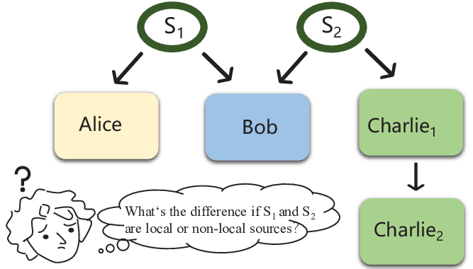
We start by recalling the description of full network non-locality in the bilocal scenario Branciard et al. 2010. Quantum network links multiple remote observers using multiple independent sources. The simplest constructure, bilocal scenario, consists of two sources and three observers, as illustrated in Fig.1. Each source has a two-particle state and distributes the qubits to the two neighboring observers. The first source ($S_{1}$) sends its qubits to Alice and Bob, and the second source ($S_{2}$) sends its qubits to Bob and Charlie₁. Without loss of generality, we assume that Alice, Bob, and Charlie₁ carry out independent measurements $\hat{A}$,$\hat{B}$, and $\hat{C}$, with corresponding binary outcomes $a,b$, and $c$ respectively. As is well known, when the joint probabilities $p(a,b,c|\hat{A},\hat{B},\hat{C})$ can be always represented as

The correlation of this network is bilocal, otherwise, it is network nonlocal (NN), where $\lambda_{i}$ ($i\in\left\{1,2\right\}$) is the local variables associated with the sources. While full network nonlocality (FNN) is strictly stronger than standard NN Pozas-Kerstjens et al. 2022, where FNN requires all links in a network to distribute nonlocal resources. For FNN, the joint probabilities $p(a,b,c|\hat{A},\hat{B},\hat{C})$ can not be represented as

It is not trivial to determine the FNN in quantum networks, which can not be determined by the most well-known network Bell test Saunders et al. 2017. Recently, Kerstjens et.al provided a method to determine FNN based on the inflation of networks Pozas-Kerstjens et al. 2022. Here we describe how to determine the FNN in an extended bilocal scenario according to Pozas-Kerstjens et al. 2022. As illustrated in Fig.1, in contrast with the standard bilocal scenario, two observers, Charlie₁ and Charlie₂, will measure their shared qubits sequentially in the extended bilocal scenario. The two separate sources are $\rho_{AB}$ and $\rho_{BC}$ respectively and the initial state of the whole system can be written as,

Different from the measurements of the standard entanglement swapping setup, Bob performs incomplete Bell state measurement on his received qubit, denoted by $\hat{B}$, with three possible outcomes $b\in\left\{0,1,2\right\}$, which corresponds to $\left|\phi^{+}\right\rangle,\left|\phi^{-}\right\rangle$, and the indiscernible between the two remaining Bell states $\left\{\psi^{+},\psi^{-}\right\}$ respectively, where $\left|\phi^{\pm}\right\rangle=\frac{1}{\sqrt{2}}(\left|00\right\rangle\pm\left|11\right\rangle)$ and $\left|\psi^{\pm}\right\rangle=\frac{1}{\sqrt{2}}(\left|01\right\rangle\pm\left|10\right\rangle)$. Wherein $\rho_{b}$ is the projective density matrix of the incomplete Bell state measurement with the outcome $b$. Alice (Charlie_m) chose two different dichotomic measurement independently which is defined as $\hat{A}\in\{\hat{A}_{i}\}$ ( $\hat{C}_{m}\in\{\hat{C}_{m,j}\}$,$m\in\left\{1,2\right\}$), with the corresponding outcomes $a_{i}\in\left\{0,1\right\}$($c_{m,j}\in\left\{0,1\right\}$). Wherein $\hat{A}_{i}$ represents the ith measurement of the observer Alice, $\hat{C}_{m,j}$ represents the jth measurement of the observer Charlie_m. Without loss of generality, these operators can be given as,

where $\sigma_{x}$ and $\sigma_{z}$ are Pauli operators. After multiple rounds of measuring process, it is easy to obtain the joint conditional probability distribution $P(a,b,c_{1},c_{2}|\hat{A},\hat{B},\hat{C}_{1},\hat{C}_{2})$. Furthermore, the joint measurement probability distribution of three different observers, whether Alice-Bob-Charlie₁ or Alice-Bob-Charlie₂ can be given by the marginal constraint of the joint probability $P(a,b,c_{1},c_{2}|\hat{A},\hat{B},\hat{C}_{1},\hat{C}_{2})$. Therefore, it is possible to determine the FNN correlation between three different observers, Alice, Bob, and Charlie_m.

According to Pozas-Kerstjens et al. 2022, the FNN can be witnessed via violations of KGT inequalities where two inequalities should be violated simultaneously,

and these average value terms can be obtained by

Then, we carefully derive the required joint measurement probabilities $P(a,b,c_{m}|\hat{A}_{i},\hat{B},\hat{C}_{m,j})$ by following the measurement process. When Bob performs incomplete BSM on the received qubits with the outcome $b$, the state of the whole system can be obtained by,

The conditional reduced system on Alice’side and Charlie’side is given by tracing out Bob’s system,

As has been mentioned, Alice carries out the strong measurement on her received qubit $\hat{A}\in\{\hat{A}_{i}\}$ with the outcome $a\in\{a_{i}\}$, the remaining system changes to,

where $U_{\hat{A}}^{a}={\textstyle\prod_{\hat{A}}^{a}}\otimes I$ and ${\textstyle\prod_{\hat{A}}^{a}}=\frac{I+(-1)^{a}\hat{A}}{2}$. Instead, Charlie₁ and Charlie₂ measure their shared qubit sequentially. Charlie₁ performs a weak measurement $\hat{C}_{1}$ on her received qubit with the quality factor $F$ and precision factor $G$, where $F$ expresses the undisturbed magnitude of quantum system after the measurement and $G$ quantifies the information gain from Charlie₁’s measurement, $G,F\in[0,1]$. A more detailed description of these two parameters of weak measurement is defined in Silva et al. 2015; Ren et al. 2019. Here we adopt the following relation between $F$ and $G$, $F^{2}+G^{2}=1$, which implies the weak measurement process with the optimal pointer Silva et al. 2015. When Charlie₁ performs a weak measurement $\hat{C}_{1}\in\{\hat{C}_{1,j}\}$ on her received qubit with the outcome $c_{1}\in\{c_{1,j}\}$, the remaining system changes to,

where $U_{\hat{C}_{m}}^{c_{m}}=I\otimes{\textstyle\prod_{\hat{C}_{m}}^{c_{m}}}$, and ${\textstyle\prod_{\hat{C}_{m}}^{c_{m}}}\in\left\{\frac{I+(-1)^{c_{m}}\hat{C}_{m,j}}{2}\right\}$. Finally, Charlie₂ performs a strong measurement $\hat{C}_{2}\in\{\hat{C}_{2,j}\}$ on her received qubit with output $c_{2}\in\{c_{2,j}\}$, and the reduced state can be expressed as

The measurement process of the extended bilocal scenario has been completely described. We can obtain the whole joint probability distribution from this equation,

The marginal probability of any combination of Alice-Bob-Charlie_m $(m\in\left\{1,2\right\})$ can be obtained from the whole joint probability distribution,

Therefore, all average values (7) depending on different measurements of any three observers can be easily calculated from (15). It is possible to check whether the KGT inequalities are violated or not.

Obviously, when $G=1$, the extended bilocal scenario regresses to the standard bilocal scenario, which is the case where Charlie₁ always performs strong measurements. Firstly, we analyze the optimal exhibition FNN in this case by investigating the maximal violation of KGT inequalities. Without loss of generality, we assume that the two remote sources in the scenario are singlet states, where $\rho_{AB}=\rho_{BC}=|\psi^{-}\rangle\langle\psi^{-}|$. Bob performs incomplete BSM with three outcomes. According to (II), the direction of each dichotomic measurement can be denoted as $\{\theta_{1}$, $\theta_{2}\}$ for Alice, and $\{\theta_{3}$, $\theta_{4}\}$ for Charlie₁. It is easy to obtain the left terms of KGT inequalities, $\mathcal{R}_{C-NS}^{1}$ and $\mathcal{R}_{NS-C}^{1}$, which can be given as,

and

Using the method of Lagrange multipliers, the maximal KGT inequalities violation, $Max\left\{min\left\{\mathcal{R}_{C-NS}^{1},\mathcal{R}_{NS-C}^{1}\right\}\right\}$, can be obtained as,

when $\theta_{1}=\frac{\pi}{2},\theta_{2}=0,\theta_{3}=-\theta_{4}$. And the maximal violation $\sqrt{13}\approx 3.6055$ can be achieved when $\theta_{3}=\mathrm{\arccos}[\frac{3}{\sqrt{13}}]$. It is larger than the previous result presented in Pozas-Kerstjens et al. 2022, which shows the violation reaches $\frac{5}{\sqrt{2}}\approx 3.5355$ when $\theta_{1}=0,\theta_{2}=\frac{\pi}{2},\theta_{3}=-\theta_{4}=\frac{\pi}{4}$ respectively. A larger violation is more friendly to the experimental demonstration.

More generally, no matter what the reason, if Charlie₁ actually performs a weak measurement rather than a strong measurement, the initial quantum system is not fully changed by the measurement process, and the corresponding initial correlation information is not completely destroyed. It allows us to explore the FNN sharing between different combinations of observations. Taking the simplest model as an example, Charlie₁ chooses two different dichotomic observables randomly, and then unbiasedly delivers the measured qubit to the Charlie₂, where the ”unbiasedly” means the received qubits by Charlie₂ equally come from any of these two different measurements by Charlie₁. In addition, Charlie₂ carries out strong measurements on the received qubits independently, and any communication is forbidden for all observers. In the extended bilocal scenario, we can investigate the FNN of Alice-Bob-Charlie_m ($m\in\left\{1,2\right\}$), or there both.

Assumed that the direction of each dichotomic measurement can be denoted as $\{\theta_{1}$, $\theta_{2}\}$ for Alice, $\{\theta_{3}$, $\theta_{4}\}$ for Charlie₁ and $\{\theta_{5}$, $\theta_{6}\}$ for Charlie₂, we can obtain the KGT expressions for Alice-Bob-Charlie_m respectively according to the discussion in Sec. II. $\mathcal{R}_{C-NS}^{1}$ and $\mathcal{R}_{NS-C}^{1}$ corresponds to Alice-Bob-Charlie₁, $\mathcal{R}_{C-NS}^{2}$ and $\mathcal{R}_{NS-C}^{2}$ corresponds to Alice-Bob-Charlie₂. These different KGT expressions can be given as,

where F and G are the quality factor and precision factor of weak measurements for Charlie₁.

We can investigate the FNN sharing by analyzing the simultaneous violation of these KGT inequalities (19-22) between Alice-Bob-Charlie₁ and Alice-Bob-Charlie₂. Inspired by the deep understanding of standard Bell nonlocality sharing Ren et al. 2019, the FNN sharing in the extended bilocal scenario may exist in two different types based on the motivation of Charlie₁, passive and active sharing Ren et al. 2019 respectively. Passive FNN sharing implies that Charlie₁ has no conscious thought of FNN sharing with subsequent observers, but only wants to achieve a maximal KGT violation of Alice-Bob-Charlie₁. While active FNN sharing means Charlie₁ wants to help the subsequent observers possess FNN as much as possible on the premise of ensuring that he has already possessed.

We discuss the possibility of passive FNN sharing at first. The pointer type of the weak measurement adopts the optimal, that is $F^{2}+G^{2}=1$, which always gives the optimal tradeoff between the information gain and disturbance Silva et al. 2015. Since Charlie₁ only wants to observe the maximal violation of KGT inequalities of Alice-Bob-Charlie₁ in the case of fixed $G$. According to the above result in Sec.III, the maximal KGT violation will be reached when $\theta_{1}=\frac{\pi}{2},\theta_{2}=0,\theta_{3}=-\theta_{4},\theta_{3}=\arccos[\frac{3}{\sqrt{13}}]$, where $\mathcal{R}_{1}=\mathcal{R}_{C-NS}^{1}=\mathcal{R}_{NS-C}^{1}=\sqrt{13}G$. Under these optimal settings, the KGT expressions for Alice-Bob-Charlie₁ are limited by the accuracy factor G.

Subsequently, Charlie₁ delivers the measured qubit to Charlie₂. Similarly, Charlie₂ will choose the optimal measurements to achieve the maximal violation of KGT inequalities of Alice-Bob-Charlie₂ under the constraint of the optimal measurement settings of Charlie₁. It is easy to obtain that the maximal violation of KGT inequalities of Alice-Bob-Charlie₂, $\mathcal{R}_{2}=Max\left\{min\left\{\mathcal{R}_{C-NS}^{2},\mathcal{R}_{NS-C}^{2}\right\}\right\}$ will achieve when $\theta_{5}=-\theta_{6}$. The KGT inequalities of Alice-Bob-Charlie₂ can be expressed as,

where $K=\frac{3}{2}(1+F-(-1+F)\cos 2\theta_{3})$, $T=1+F+(-1+F)\cos 2\theta_{3}$ and $\theta_{3}=\arccos[\frac{3}{\sqrt{13}}]$. The bound of (IV) reaches when $\theta_{5}=\arccos[\frac{K}{\sqrt{K^{2}+T^{2}}}]$.

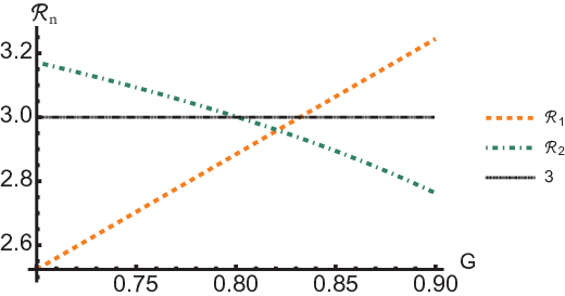
Using relations between the quality factor $F$ and the precision factor $G$, $G^{2}+F^{2}=1$, $\mathcal{R}_{1}=\sqrt{13}G$ and $\mathcal{R}_{2}=\sqrt{K^{2}+T^{2}}$ are only depend on the precision factor $G$. The passive FNN sharing can only be observed when both $\mathcal{R}_{1}$ and $\mathcal{R}_{2}$ exceed 3 simultaneously. Unfortunately, it is easy to obtain that $\mathcal{R}_{1}$ exceed 3 in the range of $G\in[0.8321,1]$, while $\mathcal{R}_{2}$ exceed 3 in the range of $G\in[0,0.8014]$. As illustrated in Fig.2, the maximal value of $Max\left\{min\left\{\mathcal{R}_{1},\mathcal{R}_{2}\right\}\right\}$ is $2.9596$, when $G=0.8208$. The simultaneous violation of KGT inequalities between Alice-Bob-Charlie₁ and Alice-Bob-Charlie₂ is impossible, the passive FNN sharing phenomenon does not exist. This property of FNN sharing is different from that of Bell nonlocal sharing Ren et al. 2019 or network nonlocal sharing Hou et al. 2022.

As opposed to passive sharing, if Charlie₁ is willing to help Charlie₂ to exhibit FNN as much as possible under the condition that the KGT inequalities from Alice-Bob-Charlie₁ can be guaranteed to be violated, it is denoted as active FNN sharing. To exhibit active FNN sharing, it is necessary to solve the question, $Max\left\{min\left\{\mathcal{R}_{C-NS}^{1},\mathcal{R}_{NS-C}^{1},\mathcal{R}_{C-NS}^{2},\mathcal{R}_{NS-C}^{2}\right\}\right\}$. Using the extreme value solution method, we obtain that the solution should satisfy $\theta_{1}=\frac{\pi}{2},\theta_{2}=0,\theta_{3}=-\theta_{4},\theta_{5}=-\theta_{6}$.

Taking these condition into $\mathcal{R}_{C-NS}^{1}$, $\mathcal{R}_{NS-C}^{1}$, $\mathcal{R}_{C-NS}^{2}$, and $\mathcal{R}_{NS-C}^{2}$, we can obtain that $\mathcal{R}_{C-NS}^{1}=\mathcal{R}_{NS-C}^{1}=\mathcal{R}_{1}$, $\mathcal{R}_{C-NS}^{2}=\mathcal{R}_{NS-C}^{2}=\mathcal{R}_{2}$, where

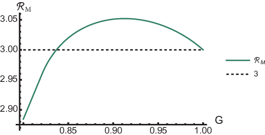
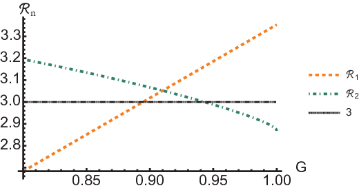
where $K=\frac{3}{2}(1+F-(-1+F)\cos 2\theta_{3})$, $T=1+F+(-1+F)\cos 2\theta_{3}$. Therefore, $\mathcal{R}_{1}$ is determined by $G$ and $\theta_{3}$, while $\mathcal{R}_{2}$ is determined by $\theta_{3}$ and $\theta_{5}$, and $G$ owing to $F^{2}+G^{2}=1$. Using the method of Lagrange multipliers, we can obtain the analytical expression of $\mathcal{R}_{M}=Max\left\{min\left\{\mathcal{R}_{1},\mathcal{R}_{2}\right\}\right\}$. But the analytical expression is too complex and too long to show here. Nevertheless, $\mathcal{R}_{M}$ as a function of $G$ can be drawn clearly as illustrated by Fig.3. $\mathcal{R}_{1}\equiv\mathcal{R}_{2}$, when $\mathcal{R}_{M}$ reaches. The simultaneous violation of KGT inequalities between Alice-Bob-Charlie₁ and Alice-Bob-Charlie₂ exists in the range of $G\in(0.84,1)$, which means the active FNN sharing can be demonstrated using weak measurements with near-maximum strength. The maximal value of $\mathcal{R}_{M}$ can reaches 3.0521, when $G=0.91$, $\theta_{3}=0.2122$ and $\theta_{5}=0.2929$. As we fixed $\theta_{3}=0.2122$ and $\theta_{5}=0.2929$, a sub-optimal simultaneous violation of KGT inequalities can be observed in the range of $G\in(0.8945,0.9431)$, where $\mathcal{R}_{1}\neq\mathcal{R}_{2}$ as illustrated in Fig.4.

In fact, the impact of noise is inevitable. It is also interesting to discuss the noise immunity of FNN or active FNN sharing in this scenario. The noise may come from many different aspects. For simplicity, we just analyze the case of imperfect sources in the network. We assume that the shared state of these sources is not a singlet state, but a Werner state $\rho(V_{i})$,

where $I$ is $2\times 2$ identity. Assuming other conditions remain constant, Charlie₁ performs strong measurements, the maximal KGT inequalities violation, $Max\left\{min\left\{\mathcal{R}_{C-NS}^{1},\mathcal{R}_{NS-C}^{1}\right\}\right\}$, can be obtained that $\mathcal{R}_{C-NS}^{1}=\mathcal{R}_{NS-C}^{1}=3V_{1}V_{2}\cos\theta_{3}+2V_{1}V_{2}\sin\theta_{3}\leq\sqrt{13}V_{1}V_{2}$. It is easy to find the violations of the KGT inequalities of Alice₁-Bob-Charlie₁ when $V\geq 0.912$, where $V=\sqrt{V_{1}V_{2}}$. Hence, the FNN can be observed if $V$ is no less than $0.912$.

Similarly, the noise immunity of the simultaneous violation of KGT inequalities between Alice-Bob-Charlie₁ and Alice-Bob-Charlie₂ can be discussed. For two Werner states as resources,

Supposed that $V=\sqrt{V_{1}V_{2}}$, we can observe the simultaneous violation of the KGT inequalities between Alice₁-Bob-Charlie₁ and Alice₁-Bob-Charlie₂ when $V\geq 0.9914$. Obviously, the active FNN sharing is too fragile to robust noise in the extended bilocal scenario.

We have deeply investigated the characterization of FNN in an extended bilocal scenario, where only one-sided sequential measurements were carried out by two observers. Initially, we exhibited the optimal FNN by the maximal violation of KGT inequality of Alice-Bob-Charlie₁, when the scenario regresses to the standard bilocal. It is shown that the maximal violation of KGT inequality can achieve $\sqrt{13}\approx 3.6055$ when $\theta_{1}=0,\theta_{2}=\frac{\pi}{2},\theta_{3}=-\theta_{4}=\mathrm{\arccos}[\frac{3}{\sqrt{13}}]$, which is larger than the previous result $\frac{5}{\sqrt{2}}\approx 3.5355$ Pozas-Kerstjens et al. 2022 with $\theta_{1}=0,\theta_{2}=\frac{\pi}{2},\theta_{3}=-\theta_{4}=\frac{\pi}{4}$. The greater the violation reaches, the easier the experiment carries out. Furthermore, the recycling of FNN as quantum resources by analyzing the FNN sharing between different combinations of observers in the extended bilocal scenario has been explored. According to the different motivations of Charlie₁ in their measurement process, we have completely discussed the possibility of two typical FNN sharing, passive FNN sharing and active FNN sharing respectively. Our results clearly demonstrated that the passive FNN sharing is impossible, as the maximal simultaneous achievement of KGT values $\mathcal{R}_{1}$ and $\mathcal{R}_{2}$ for Alice-Bob-Charlie₁ and Alice-Bob-Charlie₂ is $2.9596$, which means that the KGT inequalities cannot be simultaneously violated by these different combinations of observers Alice-Bob-Charlie_m. On the contrary, when Charlie₁ wants to help the subsequent observers possess FNN as much as possible on the premise of ensuring that he has already possessed, the simultaneous violation of KGT inequalities between Alice-Bob-Charlie₁ and Alice-Bob-Charlie₂ can be observed in the range of $G\in(0.84,1)$, which indicates the active FNN sharing exists. The simultaneous maximal violation of KGT inequalities between Alice-Bob-Charlie₁ and Alice-Bob-Charlie₂ is 3.0521, when $G=0.91$, $\theta_{3}=0.2122$ and $\theta_{5}=0.2929$. These results indicate that, compared with Bell nonlocal sharing and network nonlocal sharing, FNN sharing requires more cooperation by the intermediate observers. Moreover, we also discussed the noise immunity of FNN or active FNN sharing in this scenario.

C.R. was supported by the National Natural Science Foundation of China (Grant No. 12075245), the Natural Science Foundation of Hunan Province (2021JJ10033), Xiaoxiang Scholars Programme of Hunan Normal university.

References

- Bell (1964) J. S. Bell, Phys. Phys. Fiz 1, 195 (1964).
- Clauser et al. (1969) J. F. Clauser, M. A. Horne, A. Shimony, and R. A. Holt, Phys. Rev. Lett. 23, 880 (1969).
- Mermin (1990) N. D. Mermin, Phys. Rev. Lett. 65, 1838 (1990).
- Ardehali (1992) M. Ardehali, Phys. Rev. A 46, 5375 (1992).
- Belinskiĭ and Klyshko (1993) A. V. Belinskiĭ and D. N. Klyshko, Phys. Usp. 36, 653 (1993).
- Żukowski and Časlav (2002) M. Żukowski and B. Časlav, Phys. Rev. Lett. 88, 210401 (2002).
- Brunner et al. (2014) N. Brunner, D. Cavalcanti, S. Pironio, V. Scarani, and S. Wehner, Rev. Mod. Phys. 86, 419 (2014).
- Schrödinger (1936) E. Schrödinger, Nature(London) 138, 13 (1936).
- Freedman and Clauser (1972) S. J. Freedman and J. F. Clauser, Phys. Rev. Lett. 28, 938 (1972).
- Aspect et al. (1982) A. Aspect, J. Dalibard, and G. Roger, Phys. Rev. Lett. 49, 1804 (1982).
- Rarity and Tapster (1990) J. G. Rarity and P. R. Tapster, Phys. Rev. Lett. 64, 2495 (1990).
- Tittel et al. (1998) W. Tittel, J. Brendel, H. Zbinden, and N. Gisin, Phys. Rev. Lett. 81, 3563 (1998).
- Weihs et al. (1998) G. Weihs, T. Jennewein, C. Simon, H. Weinfurter, and A. Zeilinger, Phys. Rev. Lett. 81, 5039 (1998).
- Mair et al. (2001) A. Mair, A. Vaziri, G. Weihs, and A. Zeilinger, Nature(London) 412, 313 (2001).
- Bennett (1984) C. H. Bennett, in International Conference on Computers (1984).
- Bennett and DiVincenzo (2000) C. H. Bennett and D. P. DiVincenzo, Nature(London) 404, 247 (2000).
- Bouwmeester and Zeilinger (2000) D. Bouwmeester and A. Zeilinger, in The physics of quantum information (Springer, 2000) pp. 1–14.
- Jaeger (2007) G. Jaeger, Quantum information (Springer, 2007).
- Svetlichny (1987) G. Svetlichny, Phys. Rev. D 35, 3066 (1987).
- Mermin (1993) N. D. Mermin, Rev. Mod. Phys. 65, 803 (1993).
- Żukowski et al. (1993) M. Żukowski, A. Zeilinger, M. A. Horne, and A. K. Ekert, Phys. Rev. Lett. 71, 4287 (1993).
- Collins et al. (2002) D. Collins, N. Gisin, S. Popescu, D. Roberts, and V. Scarani, Phys. Rev. Lett. 88, 170405 (2002).
- Seevinck and Svetlichny (2002) M. Seevinck and G. Svetlichny, Phys. Rev. Lett. 89, 060401 (2002).
- Gisin and Gisin (2002) N. Gisin and B. Gisin, Phys. Lett. A 297, 279 (2002).
- Colbeck and Renner (2008) R. Colbeck and R. Renner, Phys. Rev. Lett. 101, 050403 (2008).
- Wood and Spekkens (2015) C. J. Wood and R. W. Spekkens, New J. Phys 17, 033002 (2015).
- Silva et al. (2015) R. Silva, N. Gisin, Y. Guryanova, and S. Popescu, Phys. Rev. Lett. 114, 250401 (2015).
- Mal et al. (2016) S. Mal, A. S. Majumdar, and D. Home, Mathematics-Basel 4, 48 (2016).
- Bera et al. (2018) A. Bera, S. Mal, A. Sen(De), and U. Sen, Phys. Rev. A 98, 062304 (2018).
- Ren et al. (2019) C. Ren, T. Feng, D. Yao, H. Shi, J. Chen, and X. Zhou, Phys. Rev. A 100, 052121 (2019).
- Kumari and Pan (2019) A. Kumari and A. K. Pan, Phys. Rev. A 100, 062130 (2019).
- Yao and Ren (2021) D. Yao and C. Ren, Phys. Rev. A 103, 052207 (2021).
- Cheng et al. (2021) S. Cheng, L. Liu, T. J. Baker, and M. J. W. Hall, Phys. Rev. A 104, L060201 (2021).
- Zhu et al. (2022) J. Zhu, M.-J. Hu, C.-F. Li, G.-C. Guo, and Y.-S. Zhang, Phys. Rev. A 105, 032211 (2022).
- Schiavon et al. (2017) M. Schiavon, L. Calderaro, M. Pittaluga, G. Vallone, and P. Villoresi, Quantum Sci. Technol. 2, 015010 (2017).
- Hu et al. (2018) M.-J. Hu, Z.-Y. Zhou, X.-M. Hu, C.-F. Li, G.-C. Guo, and Y.-S. Zhang, Npj Quantum Inf. 4, 1 (2018).
- Feng et al. (2020) T. Feng, C. Ren, Y. Tian, M. Luo, H. Shi, J. Chen, and X. Zhou, Phys. Rev. A 102, 032220 (2020).
- Anwer et al. (2020) H. Anwer, S. Muhammad, W. Cherifi, N. Miklin, A. Tavakoli, and M. Bourennane, Phys. Rev. Lett. 125, 080403 (2020).
- Foletto et al. (2020) G. Foletto, L. Calderaro, G. Vallone, and P. Villoresi, Phys. Rev. Research 2, 033205 (2020).
- Anwer et al. (2021) H. Anwer, N. Wilson, R. Silva, S. Muhammad, A. Tavakoli, and M. Bourennane, Quantum-Austria 5, 551 (2021).
- Branciard et al. (2010) C. Branciard, N. Gisin, and S. Pironio, Phys. Rev. Lett. 104, 170401 (2010).
- Fritz (2012) T. Fritz, J. Math. Phys. 53, 072202 (2012).
- Branciard et al. (2012) C. Branciard, D. Rosset, N. Gisin, and S. Pironio, Phys. Rev. A 85, 032119 (2012).
- Gisin et al. (2017) N. Gisin, Q. Mei, A. Tavakoli, M. O. Renou, and N. Brunner, Phys. Rev. A 96, 020304 (2017).
- Carvacho et al. (2018) G. Carvacho, F. Andreoli, L. Santodonato, M. Bentivegna, V. D’Ambrosio, P. Skrzypczyk, I. Šupić, D. Cavalcanti, and F. Sciarrino, Phys. Rev. Lett. 121, 140501 (2018).
- Tavakoli et al. (2014) A. Tavakoli, P. Skrzypczyk, D. Cavalcanti, and A. Acín, Phys. Rev. A 90, 062109 (2014).
- Saunders et al. (2017) D. J. Saunders, A. J. Bennet, C. Branciard, and G. J. Pryde, Sci. Adv 3 (2017).
- Tavakoli et al. (2021) A. Tavakoli, N. Gisin, and C. Branciard, Phys. Rev. Lett. 126 (2021).
- Tavakoli et al. (2022) A. Tavakoli, A. Pozas-Kerstjens, M.-X. Luo, and M.-O. Renou, Rep. Prog. Phys. 85, 056001 (2022).
- Żukowski et al. (1995) M. Żukowski, A. Zeilinger, and H. Weinfurter, Ann. N. Y. Acad. Sci. 755 (1995).
- Bose et al. (1999) S. Bose, V. Vedral, and P. L. Knight, Phys. Rev. A 60, 194 (1999).
- Pozas-Kerstjens et al. (2022) A. Pozas-Kerstjens, N. Gisin, and A. Tavakoli, Phys. Rev. Lett. 128 (2022).
- Hou et al. (2022) W. Hou, X. Liu, and C. Ren, Phys. Rev. A 105, 042436 (2022).
- Wang et al. (2022) J. Wang, Y. Wang, L. Wang, and Q. Chen, arXiv:2206.03100 (2022).