Data-Driven Inverse of Linear Systems
and Application to Disturbance Observers
Abstract
This work develops a data-based construction of inverse dynamics for LTI systems. Specifically, the problem addressed here is to find an input sequence from the corresponding output sequence based on pre-collected input and output data. The problem can be considered as a reverse of the recent use of behavioral approach, in which the output sequence is obtained for a given input sequence by solving an equation formed by pre-collected data. The condition under which the problem gives a solution is investigated and turns out to be -delay invertibility of the plant and a certain degree of persistent excitation of the data input. The result is applied to form a data-driven disturbance observer. The plant dynamics augmented by the data-driven disturbance observer exhibits disturbance rejection without the model knowledge of the plant.
I Introduction
Seminal work of the behavioral approach [1] for dynamic systems has been receiving growing attention in recent years [2, 3, 4]. Instead of using matrices , , and for linear dynamics, which are often obtained from the first principle on the target dynamics, the behavioral approach uses a set of equations to determine if a pair of input and output belongs to the target dynamics. The equations involve Hankel matrices for linear dynamics, which are obtained by input/output trajectories that satisfy a condition of persistently exciting. This approach suits when data are available but applying the first principle for modeling is not straightforward. Recent advances in this area include [5, 6, 3, 7].
Particularly, as given in [8], the fundamental result of this approach is that we can determine a future output for a given input using Hankel matrices built by using previously collected input and output data. No identification of system matrices (typically , , , ) is necessary. A question that this paper is concerned is the inverse of what is just described: can we determine the input that generated a given output using previously collected input and output data? In other words, the question pertains to finding conditions and methods how we can build an inverse dynamics of the given system using collected data. If this is successfully carried out, an immediate application is to build a disturbance observer [9, 10] with data, that identifies the disturbance that affected the output. Another application is to find a suitable constrained input that yields an output close to the desired output under constraints.
Similar question has been asked and answered in [11, 8]. However, the result is restricted to the case where is invertible. This work does not assume the invertibility of . Instead the notion of -delay invertibility is invoked from the literature [12].
This paper is organized as follows: Section II provides a brief review of the invertibility of discrete-time LTI systems. Section III gives main results. An application of disturbance observer is given in Section IV. Section V concludes the paper.
II Review of LTI System Invertibility
Consider a discrete-time linear-time-invariant system
| (1a) | ||||
| (1b) | ||||
where is the state, is the input, is the output, and is the discrete time index. Then the transfer function matrix of given system (1) is given by .
Definition 1 (see [12]).
A proper transfer function matrix is an -delay inverse system for given system (1), where is a nonnegative integer, if
| (2) |
Note that is an transfer function matrix and is a transfer function matrix. Thus, a necessary condition for (2) is that .
Definition 2 (see [12]).
The system (1) is invertible if it has an -delay inverse for some finite . The least integer for which an -delay inverse exists will be called the inherent delay of the invertible system and is denoted by .
For single input and single output systems of (1), the inherent delay is the relative degree.
Define, for an integer ,
| (3) | ||||
In addition, define . Then, the following theorem gives the necessary and sufficient condition for the existence of an -delay inverse for the system of (1).
Theorem 1 (see [12]).
The following are equivalent:
- 1.
The system (1) has an -delay inverse.
- 2.
There exists such that
(4) where .
- 3.
The rank of the matrix is .
As a result of Theorem 1, if the system has -delay inverse, then the first columns of are independent.
III Data-based Construction of Inverse Systems
We introduce notations commonly used in the literature for data-driven system and control. For a given signal , , and , let be defined by
Using the vectors and , the system of (1) can be written as
| (5) |
where the matrix is defined by
| (6) |
When the -delay inverse exists for the system of (1), there exists an matrix satisfying
Such a matrix exists due to Rouché-Capelli theorem [13] with the fact that
which follows from the fact that the first columns of are independent. Pre-multiplying to both sides of (5) yields
| (7) |
which represents the input by the state and sequence of outputs. State update equation with respect to is obtained by substituting (7) in (1a). Then, the following dynamics is obtained:
| (8a) | ||||
| (8b) | ||||
where , , , and .
In order to provide more specific arguments, we first remind readers of Hankel matrix and the notion of persistent excitation (PE) for a signal . Denote by the dimensional Hankel matrix constructed using the values of :
The notion of persistency of excitation of a segment from a signal is defined as follows.
Definition 3 (see [1]).
The vector from signal is persistently exciting of order if the matrix has full row rank.
As hinted by (8), data-based construction of inverse dynamics may involve input and output sequences of different length.
Lemma 1.
Now, for some and , denote the input and output data collected from an experiment for the system (1) by and , respectively.
Lemma 2.
Proof.
Let and be a trajectory of (1). Then, by Lemma 1, there exists such that the pair and is a trajectory of (1). Then, by [5, Theorem 1] there exists such that
| (10) |
Hence (9) is satisfied. Conversely, let and satisfy (9) for some . Set the subsequent sequence of as
| (11) |
Then, and satisfy (10). Again due to [5, Theorem 1] the pair is the trajectory of (1), and due to Lemma 1, the pair and is a trajectory of (1). ∎
Denote by , , and the following four Hankel matrices formed by the data , for some and satisfying
Lemma 3.
Proof.
Denote by , and define for the simplicity of derivation. First, we show that is determined by and by (7) and (8) as
Again using (3), (6), and (8), is determined by and as
| (13) |
where
and implies the left-inverse of a matrix. Finally, let be a matrix that include the identity matrix of size from its -th column and all other elements are zero. Then, it is easily seen that
| (14) |
where . Therefore, is determined by . Combining (13) and (14), we arrive that linearly depends on , and . Therefore, (12) follows. ∎
Now we state the main result of this paper.
Theorem 2.
Let the system of (1) be controllable, observable and have an -delay inverse with . Assume that be greater than or equal to the observability index of (1) and is PE of order . Then, for any trajectory and of (1) where is arbitrary, the input sequence is uniquely determined by
| (15) |
where is a solution of
| (16) |
Proof.
We first claim that (16) always has a solution. Since and are (different length) trajectory of (1), there exists a long sequence that satisfies
| (17) |
Theorem 2 provides a foundation to answer the question posed in Introduction, i.e., determining the input that generated a given output using previously collected data, since it states that long input is uniquely determined for any pair and . Figure 1 illustrates this with color coded signals when , and . Signals in black are required to determine the signal in red.

The necessity of long pair of previous and is for the system state identification. From this perspective, an interpretation of the theorem is given as follows. Any vector belonging to
contains the information of the state , so that the set
is a collection of all possible -long input and -long output sequences starting from . Thus, any observed must belong to this set, i.e., there exists and
This is identified by solving (16). The corresponding is obviously given as in (15) and unique.
The result of Theorem 2 is written in the form of algorithm. See Algorithm 1.
To initiate Algorithm 1, and must be obtained. If the system is initially at rest, both can be set to zeros. An example is provided.
Example 1.
As an example, we consider the system of (1) with
| (19a) | ||||
| (19b) | ||||
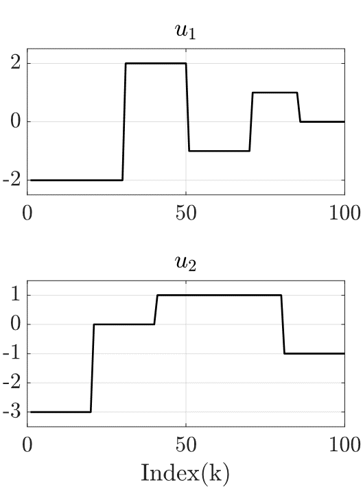
The system has -inverse with . Applying as shown in Figure 2(a) to the system with yields as shown in Figure 2(b).


To apply Algorithm 1, we set , , and , and make Hankel matrices with data generated by a 30 long random input sequence satisfying PE of order . Assuming the system initially at rest, Algorithm 1 begins iteration at time with , and the first input to the algorithm is . Denoting the outcome of Algorithm by at time , we obtain , which is shown in Figure 3 in red.

Clear, and are identical with step delay.
Note that is computed in batches of length . Iteration gives .
Algorithm 1 receives as an input and computes at a time. This may be cumbersome to implement for real-time applications. We provide Algorithm 2 tailored for real-time application. Here, the input is modified to use available up to the current instance and compute of length 1.
Example 2.
Algorithm 2 is used with and . Figure 4 shows the input and output sequence. Figure 5 shows the along with . Indeed they are identical with one step delay.


Example 3.
The proposed inversion of a linear system can also be used for finding a constrained input that yields a desired output. Consider a desired output and an input constraint set . Suppose that we want to find a constrained input sequence at time when the previous records of input and output are available. Then, solve the minimization problem for :
| subject to | |||
and set .
IV Application to Disturbance Observer
Consider the block diagram of Figure 6, where is the plant and the block ‘DBINV’ is the data-based inversion block of implemented by Algorithm 2. The signals , , , are, respectively, command input, output, disturbance, and the actual input to the plant. Note that the transfer function from to is
| (21) |
where , , and are -transform of the corresponding signals, which can also be seen from the figure by
From (21) it is seen that, when is slowly varying, the effect of is approximately removed from the input. This is exactly the idea of the model-based disturbance observer [10]. In this sense, we refer the proposed structure as data-driven disturbance observer.

Example 4.
Consider the block diagram of Figure 6 where a realization of is given by the system of (19). We assume that the signal is the same as the signal shown in Figure 2(a) and the signal is given in Figure 7(a). The corresponding output is shown in Figure 7(b). Clearly, the effect of disturbance is removed after some transients.


The simulation results agree with the derivation in (21) and we emphasize that no information of is directly used, and thus, the term of data-driven disturbance observer is justified.
V Conclusions
A data-based construction of inverse dynamics has been developed for discrete-time LTI systems. The notion of -delay inverse is invoked from the literature, and it is combined with the system description method from behavioral approach. The outcome is data-based representation of inverse dynamics, which is similar to that of LTI systems, but differs in that input is estimated with some delay. The result is applied to build disturbance observers from no system information but collected input and output data that satisfy a level of persistency of excitation condition. Applications and extension this result seem to be immense.
References
- [1] J. C. Willems, P. Rapisarda, I. Markovsky, and B. L. M. De Moor, “A note on persistency of excitation,” Systems and Control Letters, vol. 54, no. 4, pp. 325–329, 2005.
- [2] L. Huang, J. Coulson, J. Lygeros, and F. Dörfler, “Data-enabled predictive control for grid-connected power converters,” in the Proceedings of Conference on Decision and Control (CDC), pp. 8130-8135, 2019.
- [3] J. Coulson, J. Lygeros, and F. Dörfler, “Data-enabled predictive control: In the shallows of the DeePC,” in the Proceedings of European Control Conference (ECC) pp. 307-312, 2019.
- [4] P. G. Carlet, A. Favato, S. Bolognani, and F. Dörfler, “Data-driven predictive current control for synchronous motor drives,” in the Proceedings of Energy Conversion Congress and Exposition (ECCE), pp. 5148-5154, 2020.
- [5] H. J. van Waarde, C. De Persis, M. K. Camlibel, and P. Tesi, “Willems’ fundamental lemma for state-space systems and its extension to multiple datasets,” IEEE Control Systems Letters, vol. 4, no. 3, pp. 602-607, 2020.
- [6] C. De Persis and P. Tesi, “Formulas for data-driven control: Stabilization, optimality, and robustness,” IEEE Transactions on Automatic Control, vol. 65, no. 3, pp. 909–924, 2020.
- [7] F. Dörfler, J. Coulson, and I. Markovsky, “Bridging direct & indirect data-driven control formulations via regularizations and relaxations,” IEEE Transactions on Automatic Control, 2022.
- [8] I. Markovsky, J. C. Willems, S. Van Huffel, and B. De Moor, Exact and Approximate Modeling of Linear Systems: A Behavioral Approach. Philadelphia, PA, USA: SIAM, Mar. 2006.
- [9] K. Ohishi, M. Nakao, K. Ohnishi, and K. Miyachi, “Microprocessor-controlled DC motor for load-insensitive position servo system,” IEEE Transactions on Industrial Electronics, vol. IE-34, no. 1, pp. 44–49, 1987.
- [10] H. Shim, “Disturbance Observers,” In: Baillieul, J., Samad, T. (eds) Encyclopedia of Systems and Control, Springer, London, 2020. https://doi.org/10.1007/978-1-4471-5102-9_100068-1
- [11] I. Markovsky and P. Rapisarda, “Data-driven simulation and control,” International Journal of Control, vol. 81, no. 12, pp. 1946-1959, 2008.
- [12] M. Sain, J. Massey. “Invertibility of linear time-invariant dynamical systems.” IEEE Transactions on automatic control, vol. 14, no. 2, pp. 141-149, 1969.
- [13] https://en.wikipedia.org/wiki/Rouche-Capelli_theorem