Spade: A Real-Time Fraud Detection Framework on Evolving Graphs (Complete Version)
Abstract.
Real-time fraud detection is a challenge for most financial and electronic commercial platforms. To identify fraudulent communities, , one of the largest technology companies in Southeast Asia, forms a graph from a set of transactions and detects dense subgraphs arising from abnormally large numbers of connections among fraudsters. Existing dense subgraph detection approaches focus on static graphs without considering the fact that transaction graphs are highly dynamic. Moreover, detecting dense subgraphs from scratch with graph updates is time consuming and cannot meet the real-time requirement in industry. To address this problem, we introduce an incremental real-time fraud detection framework called . can detect fraudulent communities in hundreds of microseconds on million-scale graphs by incrementally maintaining dense subgraphs. Furthermore, supports batch updates and edge grouping to reduce response latency. Lastly, provides simple but expressive APIs for the design of evolving fraud detection semantics. Developers plug their customized suspiciousness functions into which incrementalizes their semantics without recasting their algorithms. Extensive experiments show that detects fraudulent communities in real time on million-scale graphs. Peeling algorithms incrementalized by are up to a million times faster than the static version.
PVLDB Reference Format:
PVLDB, 16(3): XXX-XXX, 2022.
doi:XX.XX/XXX.XX
††
This work is licensed under the Creative Commons BY-NC-ND 4.0 International License. Visit https://creativecommons.org/licenses/by-nc-nd/4.0/ to view a copy of this license. For any use beyond those covered by this license, obtain permission by emailing info@vldb.org. Copyright is held by the owner/author(s). Publication rights licensed to the VLDB Endowment.
Proceedings of the VLDB Endowment, Vol. 16, No. 3 ISSN 2150-8097.
doi:XX.XX/XXX.XX
1. Introduction
Graphs have been found in many emerging applications, including transaction networks, communication networks and social networks. The dense subgraph problem is first studied in (goldberg1984finding) and is effective for link spam identification (gibson2005discovering; beutel2013copycatch), community detection (dourisboure2007extraction; chen2010dense) and fraud detection (hooi2016fraudar; chekuri2022densest; shin2016corescope). Standard peeling algorithms (tsourakakis2015k; hooi2016fraudar; bahmani2012densest; chekuri2022densest; boob2020flowless) iteratively peel the vertex that has the smallest connectivity (e.g., vertex degree or sum of the weights of the adjacent edges) to the graph. Peeling algorithms are widely used because of their efficiency, robustness, and theoretical worst-case guarantee. However, existing peeling algorithms (hooi2016fraudar; tsourakakis2015k; charikar2000greedy) assume a static graph without considering the fact that social and transaction graphs in online marketplaces are rapidly evolving in recent years. One possible solution for fraud detection on evolving graphs is to perform peeling algorithms periodically. We take ’s fraud detection pipeline as an example.


Fraud detection pipeline in (Figure 1). is one of the largest technology companies in Southeast Asia and offers digital payments and food delivery services. On the ’s e-commerce platform, 1) the transactions form a transaction graph . 2) updates the transaction graphs periodically . Our experiments show that it takes s to carry out () (hooi2016fraudar) on a transaction graph with M vertices and M edges. Therefore, we can execute fraud detection every seconds. 3) The dense subgraph detection algorithm and its variants are used to detect fraudulent communities. 4) After identifying the fraudsters, the moderators ban or freeze their accounts to avoid further economic loss. A classic fraud example is customer-merchant collusion. Assume that provides promotions to new customers and merchants. However, fraudsters create a set of fake accounts and do fictitious trading to use the opportunity of promotion activities to earn the bonus. Such fake accounts (vertices) and the transactions among them (edges) form a dense subgraph.
Example 1.0.
Consider the transaction graph in Figure 2, where a vertex is a user or a store, and an edge represents a transaction. Suppose a fraudulent community is identified at time and a normal user becomes a fraudster and participates in suspicious activities at . Applying peeling algorithms at , the new fraudster is detected at . However, many new suspicious activities have occurred during the time period that could cause huge economic losses.
As reported in recent studies (dailyreport; ye2021gpu), of the traffic to e-commerce portals are malicious bots in 2018. Fraud detection is challenging since many fraudulent activities occur in a very short timespan. Hence, identifying fraudsters and reducing response latency to fraudulent transactions are key tasks in real-time fraud detection.
| (charikar2000greedy) | (gudapati2021search) | (hooi2016fraudar) | ||
|---|---|---|---|---|
| Dense subgraph detection | ✓ | ✓ | ✓ | ✓ |
| Accuracy guarantees | ✓ | ✓ | ✓ | ✓ |
| Weighted graph | ✗ | ✓ | ✓ | ✓ |
| Incremental updates | ✗ | ✗ | ✗ | ✓ |
| Edge reordering | ✗ | ✗ | ✗ | ✓ |
To address real-time fraud detection on evolving graphs, a better solution would be to incrementally maintain dense subgraphs. There are two main challenges of incremental maintenance. First, operational demands require that fraudsters should be identified in milliseconds in industry. Maintaining the dense subgraph incrementally in such a short timespan is challenging. Second, fraud semantics continue to evolve and it is not trivial to incrementalize each of them. Implementing a correct and efficient incremental algorithm is, in general, a challenge. It is impractical to train all developers with the knowledge of incremental graph evaluation. To the best of our knowledge, there are no generic approaches to minimize the cost of incremental peeling algorithms. Motivated by the challenges, we design a real-time fraud detection framework, named to detect fraudulent communities by incrementally maintaining dense subgraphs. The comparison between and the previous algorithms (dense subgraphs () (charikar2000greedy), dense weighted subgraph () (gudapati2021search) and () (hooi2016fraudar)) is summarized in Table 1.
Contributions. In this paper, we focus on incremental peeling algorithms. In summary, this paper makes the following contributions.
- (1)
We build three fundamental incremental techniques for peeling algorithms to avoid detecting fraudulent communities from scratch. inspects the subgraph that is affected by graph updates and reorders the peeling sequence incrementally, which theoretically guarantees the accuracy of the worst case.
- (2)
enables developers to design their fraud semantics to detect fraudulent communities by providing the suspiciousness functions of edges and vertices. We show that a variety of peeling algorithms can be incrementalized in (Section 3) including , and .
- (3)
We conduct extensive experiments on with datasets from industry. The results show that speeds up fraud detection up to orders of magnitude since minimizes the cost of incremental maintenance by inspecting the affected area. Furthermore, the latency of the response to fraud activities can be significantly reduced. Lastly, once a user is spotted as a fraudster, we identify the related transactions as potential fraud transactions and pass them to system moderators. Up to potential fraud transactions can be prevented.
Organization. The rest of this paper is organized as follows: Section 2 presents the background and the problem statement. We introduce the framework of in Section 3 and three incremental peeling algorithms in Section 4. Section 5 reports on the experimental evaluation. After reviewing related work in Section 6, we conclude in Section 7.
2. Background
2.1. Preliminary
| Notation | Meaning |
|---|---|
| / | a transaction graph / updates to graph |
| the graph obtained by updating to | |
| / | the weight on vertex / on edge |
| the sum of the suspiciousness of induced subgraph | |
| the suspiciousness density of vertex set | |
| peeling weight, i.e., the decrease in by removing from | |
| a peeling algorithm | |
| the peeling sequence order w.r.t. | |
| the vertex set returned by a peeling algorithm | |
| the optimal vertex set, i.e., is maximized |
Graph . We consider a directed and weighted graph , where is a set of vertices and is a set of edges. Each edge has a nonnegative weight, denoted by . We use to denote the neighbors of .
Induced subgraph. Given a subset of , we denote the induced subgraph by , where . We denote the size of by .
Density metrics . We adopt the class of metrics in previous studies (hooi2016fraudar; gudapati2021search; charikar2000greedy), , where is the total weight of , i.e., the sum of the weight of and :
| (1) |
The weight of a vertex measures the suspiciousness of user , denoted by (). The weight of the edge measures the suspiciousness of transaction , denoted by . Intuitively, is the density of the induced subgraph . The larger is, the denser is.
Graph updates . We denote the set of updates to by . We denote the graph obtained by updating to as . Since transaction graphs continue to evolve, we consider edge insertion rather than edge deletion. Therefore, . Specifically, we consider two types of updates, edge insertion (i.e., ) and edge insertion in batch (i.e., ).
2.2. Peeling algorithms
2
() return and
Peeling algorithms () are widely used in dense subgraph mining (hooi2016fraudar; tsourakakis2015k; charikar2000greedy). They follow the execution paradigm in Algorithm 1 and differ mainly in density metrics. They are categorized to three categories: unweighted (charikar2000greedy), edge-weighted (gudapati2021search) and hybrid-weighted (hooi2016fraudar).
Peeling weight. Specifically, we use to indicate the decrease in the value of when the vertex is removed from a vertex set , i.e., the peeling weight. Previous work (hooi2016fraudar) formalizes as follows:
| (2) |
Peeling sequence. We use to denote the vertex set after -th peeling step. Initially, the peeling algorithms set . They iteratively remove a vertex from , such that is maximized (Line 11). The process repeats recursively until there are no vertices left. This leads to a series of sets over , denoted by of sizes . Then (), which maximizes the density metric , is returned, denoted by . For simplicity, we denote . Instead of maintaining the series , we record the peeling sequence such that .
Example 2.0.
Consider the graph in Figure 3. is peeled since its peeling weight is the smallest among all vertices. Similarly, will be peeled accordingly. Therefore, the peeling sequence is .
Complexity and accuracy guarantee. In Algorithm 1, Min-Heap is used to maintain the peeling weights, the insertion cost is . There are at most insertions. Therefore, the complexity of Algorithm 1 is . We denote the vertex set that maximizes by . Previous studies (khuller2009finding; hooi2016fraudar; charikar2000greedy) conclude that:
Lemma 2.2.
Let be the vertex set returned by the peeling algorithms and be the optimal vertex set, .
Although peeling algorithms are scalable and robust, we remark that these algorithms are proposed for static graphs, which takes several minutes on million-scale graphs. For evolving graphs, computing from scratch is still time-consuming, which cannot meet the real-time requirement. Moreover, it is not trivial to design incremental algorithms for peeling algorithms. In this paper, we investigate an auto-incrementalization framework for peeling algorithms.
Problem definition. Given a graph , a peeling algorithm , and the peeling result of on , , our problem is to efficiently identify the result of on , , where is the graph updates.

3. The Framework
In this section, we present an overview of our proposed framework and sample APIs. Subsequently, we demonstrate some examples on how to implement different peeling algorithms with .

3.1. Overview of and APIs
We follow two design goals to satisfy operational demands.
- •
Programmability. We provide a set of user-defined APIs for developers to develop their dense subgraph-based semantics to detect fraudsters. Moreover, can auto-incrementalize their semantics without recasting the algorithms.
- •
Efficiency. allow efficient and scalable fraud detection on evolving graphs in real-time.
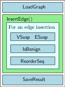
Architecture of . Figure 4 shows the architecture of and the workflow of an edge insertion. automatically incrementalizes peeling algorithms with the user-defined suspiciousness functions. To avoid computing from scratch on evolving graphs, the engine of maintains the fraudulent community incrementally with an edge update (Section 4.1). Batch execution is developed to improve the efficiency of handling edge updates in batch (Section 4.2). The updated fraudulent community is identified in real time and returned to the moderators for further analysis. Given an edge insertion, the workflow of contains the following components:
- •
and . Given a new vertex/edge, these components are responsible for deciding the suspiciousness of the endpoint of the edge or the edge with a user-defined strategy.
- •
. This component is responsible for deciding whether a new edge is benign (Section 4.3). If the edge is benign, it is inserted into an edge vector pending reordering; otherwise, peeling sequence reordering is triggered immediately for the edge buffer with this new edge.
- •
. This component is responsible for incrementally maintaining the peeling sequence and deciding the new fraudulent community with the graph updates detailed in Section 4.
APIs and data structure (Listing 1). We provide APIs for developers to customize and deploy their peeling algorithms for different application requirements. Developers can customize and to develop their fraud detection semantics. We design two APIs for edge insertion, namely and . The function spots the fraudulent community on the current graph. and are two built-in APIs which are transparent to developers. They are activated when new edges are inserted. uses the adjacency list to store the graph. Two vectors _seq and _weight are used to store the peeling sequence and the peeling weights.
Characteristic of density metrics. We next formalize the sufficient condition of the density metrics that can be supported by .
Property 3.1.
If 1) is an arithmetic density, i.e., , 2) , and 3) , then is supported by .
The correctness is satisfied since correctly returns the peeling sequence order (detailed in Section 4). We also characterize the properties of these popular density metrics in Appendix E of (techreport).
Instances. We show that popular peeling algorithms are easily implemented and supported by , e.g., (charikar2000greedy), (gudapati2021search) and (hooi2016fraudar). We take as an example and leave the discussion of the other instances in the Appendix F of (techreport). To resist the camouflage of fraudsters, Hooi et al. (hooi2016fraudar) proposed to weight edges and set the prior suspiciousness of each vertex with side information. Let . The density metric of is defined as follows:
| (3) |
To implement on , users only need to plug in the suspiciousness function for the vertices by calling and the suspiciousness function for the edges by calling . Specifically, 1) is a constant function, i.e., given a vertex , and 2) is a logarithmic function such that given an edge , , where is the degree of the object vertex between and , and is a small positive constant (hooi2016fraudar).
Developers can easily implement customized peeling algorithms with , which significantly reduces the engineering effort. For example, users write only about lines of code (compared to about lines in the original (hooi2016fraudar)) to implement .
4. Incremental peeling algorithms
In this section, we propose several techniques to incrementally identify fraudsters by reordering the peeling sequence with graph updates, i.e., the peeling sequence on , denoted by .
4.1. Peeling sequence reordering with edge insertion
Given a graph , the peeling sequence on and the graph updates , where , returns the peeling sequence on .
Vertex insertion. Given a new vertex , we insert it into the head of the peeling sequence and initialize its peeling weight by .
Insertion of an edge . Without loss of generality, we assume and denote the weight of by . Given an edge insertion , we observe that a part of the peeling sequence will not be changed. We formalize the finding as follows.
Lemma 4.1.
.
Due to space limitations, all the proofs in this section are presented in Appendix A of (techreport).
Affected area () and pending queue (). Given updates to graph and an incremental algorithm , we denote by the subgraph inspected by in that indicates the necessary cost of incrementalization. Moreover, we construct a priority queue for the vertices pending reordering in ascending order of the peeling weights.
Incremental algorithm (). initializes an empty vector for the updated peeling sequence and append to due to the Lemma 4.1. We iteratively compare 1) the head of , denoted by and 2) the vertex in the peeling sequence , where . The corresponding peeling weights are denoted by and . We consider the following three cases:
Case 1. If , we pop the from and insert it to . Then we update the priorities in for the neighbors of , .
Case 2. If and or , we insert into . The peeling weight is , .
Case 3. If and and , we insert to , .
We repeat the above iteration until is empty.

Example 4.0.
Consider the graph in Figure 3 and its peeling sequence . Suppose that a new edge is inserted into and its weight is as shown in the LHS of Figure 5. The reordering procedure is presented in the RHS of Figure 5. is pushed to the pending queue . Since the peeling weight of the next vertex in , , is the smallest, it will be inserted directly into . Since , we recover its peeling weight and push it into . Since the peeling weights of and are smaller than those of , they will pop out of and insert into . Once is empty, the rest of the vertices, and , in are appended to directly. Therefore, the reordered peeling sequence is .
Remarks. If the peeling weight of is greater than that of the head of (i.e., ), then has the smallest peeling weight among . We formalize this remark as follows.
Lemma 4.3.
If , .
Correctness and accuracy guarantee. In Case 1 of , if , is chosen to insert to since it has the smallest peeling weight due to Lemma 4.3. In Case 3 of , is the smallest peeling weight and is chosen to insert to . The peeling sequence is identical to that of , since in each iteration the vertex with the smallest peeling weight is chosen. The accuracy of the worst-case is preserved due to Lemma 2.2.
Time complexity. The complexity of the incremental maintenance is . The complexity is bounded by and is small in practice.
4.2. Peeling sequence reordering in batch

Since the peeling sequence reordering by early edge insertions could be reversed by later ones, some reorderings are stale and duplicate. Suppose that the insertion is a subgraph . A direct way to reorder the peeling sequence is to insert the edges one by one. The complexity is which is time consuming. To reduce the amount of stale computation, we propose a peeling sequence reordering algorithm in batch.

Example 4.0.
Consider a fraudulent community, , identified by the peeling algorithm in Figure 7. and are two normal users. Suppose that they have the same peeling weight and that is peeled before . When a new transaction \raisebox{-0.9pt}{1}⃝ is generated, we should reorder and by exchanging their positions. When \raisebox{-0.9pt}{2}⃝ and \raisebox{-0.9pt}{3}⃝ are inserted, positions of and will be re-exchanged. However, if we reorder the sequence in batch with the last transaction \raisebox{-0.9pt}{4}⃝, we are not required to change the positions of and .
2
3
4
color its neighbors () gray
while is not empty do 6
update the priorities of in
else 8
color its neighbors gray
else // Case 2(b) : is white 10
append to , where is the next black vertex
11
Peeling weight recovery. Given a vertex and a set of vertex (, i.e., ), the peeling weight can be calculated by .
Vertex sorting. Intuitively, the increase in peeling weight of does not change the subsequence of due to Lemma 4.1. We sort the vertices in by the indices in the peeling sequence. Then we reorder the vertices in ascending order of the indices in . For simplicity, we color the vertices in black, affected vertices (i.e., vertices pending reordering) gray and unaffected vertices white.
Incremental maintenance in batch (Algorithm 2 and Figure 6). We initialize a pending queue to maintain the vertices pending reordering (Line 2). Iteratively, we add the vertex to and color its neighbors gray (Line 2-2). If is not empty, we compare the peeling weight of the vertex () with the peeling weight of the head of , . We consider the following two cases as shown in Figure 6. Case 1: If , we pop from , insert it to and update the priorities of its neighbors in (Line 2-2); Case 2(a): if and is gray or black, we recover its peeling weight in and insert it to . Then we color the vertices in gray (Line 2-2); otherwise Case 2(b): if and is white, we insert to directly (Line 2-2). We repeat the above procedure until the pending queue is empty. Then we append to , where is the next vertex in . We insert into and repeat the reordering until there is no black vertex. The correctness and accuracy guarantee are similar to those of peeling sequence reordering with edge insertion. Due to space limitations, we present them in Appendix D of (techreport).
Complexity. The time complexity of Algorithm 2 is which is bounded by .
4.3. Peeling sequence reordering with edge grouping
Update steam . In a transaction system, the edge updates are coming in a stream manner (i.e., a timestamp on each edge) which is denoted by . Formally, we denote it by where is the timestamp on the edge .
Latency of activities . Suppose that is a labeled fraudulent activity which is generated at and is responded/inserted at . The latency of is . Given an update stream , the latency of fraudulent activities is defined as follows.
| (4) |
Prevention ratio . If a fraudster is identified, we ban the following related transactions to prevent economic loss. We denote the ratio of suspicious transactions prevented to all suspicious transactions by .
Example 4.0.
Consider an update steam in Figure 8. () are a set of labeled fraudulent transactions and () are their timestamps. Regarding the reordering in batch, the new transactions are queueing until the size of the queue is equal to the batch size. The reordering is triggered at and finished at . Therefore, they are inserted at The queueing time for each edge is while the latency is . Suppose the fraudster is identified at , the prevention ratio is .
aims to reduce and increase as much as possible. In Figure 8, if the reordering is triggered at and responded at , the following fraudulent activities can be prevented.
Intuitively, some transactions are generated by normal users (benign edges), while others are generated by potential fraudsters (urgent edges). groups the benign edges and reorders the peeling sequence in batch. It can both improve the performance of reordering and reduce the latency of the response to potential fraudulent transactions. We define the benign and urgent edges as follows.
Definition 4.0.
Given an edge and its weight , if or , is an urgent edge; otherwise is a benign edge.
Given a benign edge insertion , neither nor belongs to the densest subgraph (Lemma 4.7). And the insertion cannot produce a denser fraudulent community by peeling algorithms (Lemma 4.8).
Lemma 4.7.
Given an edge , if is a benign edge, after the insertion of , and .
We denote the vertex subset returned after reordering by .
Lemma 4.8.
Given a benign edge insertion, at least one of the following two conditions is established: 1) and ; and 2) .
Therefore, we postpone the incremental maintenance of the peeling sequence for benign edges which provide two benefits. First, we can perform a batch update that avoids stale computation. Second, an urgent edge insertion, which is caused by a potential fraudster, triggers incremental maintenance immediately. These fraudsters are identified and reported to the moderators in real time.

Edge grouping. We next present the paradigm of peeling sequence reordering by edge grouping. We first initialize an empty buffer for the updates (Line 3). When an edge enters, we insert it into . If is an urgent edge, we incrementally maintain the peeling sequence by Algorithm 2 and clear the buffer (Line 3-3).
for do 2
if is an urgent edge then 3
5. Experimental Evaluation
Our experiments are run on a machine that has an X5650 CPU, GB RAM. The implementation is made memory-resident and implemented in C++. All codes are compiled by GCC-9.3.0 with -.
| Datasets | avg. degree | Increments | Type | ||
|---|---|---|---|---|---|
| Grab1 | 3.991M | 10M | 5.011 | 1M | Transaction |
| Grab2 | 4.805M | 15M | 6.243 | 1.5M | Transaction |
| Grab3 | 5.433M | 20M | 7.366 | 2M | Transaction |
| Grab4 | 6.023M | 25M | 8.302 | 2.5M | Transaction |
| Amazon (mcauley2013hidden) | 28K | 28K | 2 | 2.8K | Review |
| Wiki-vote (leskovec2010signed) | 16K | 103K | 12.88 | 10.3K | Vote |
| Epinion (leskovec2010signed) | 264K | 841K | 6.37 | 84.1K | Who-trust-whom |
| Peeling algorithms (seconds) | () | () | () | K () | K () | |||||||||||||
|---|---|---|---|---|---|---|---|---|---|---|---|---|---|---|---|---|---|---|
| Datasets | ||||||||||||||||||
| Grab1 | 6517 | 17469 | 6 | 3117 | 11613 | 6 | 519 | 1983 | 6 | 108 | 281 | 6 | 5 | 10 | 1 | |||
| Grab2 | 17 | 20 | 16 | 6604 | 18413 | 8 | 3484 | 11280 | 8 | 634 | 1782 | 8 | 138 | 249 | 8 | 7 | 8 | 2 |
| Grab3 | 23 | 27 | 22 | 6716 | 18862 | 11 | 3864 | 10892 | 11 | 750 | 1560 | 10 | 186 | 211 | 10 | 8 | 7 | 2 |
| Grab4 | 27 | 28 | 28 | 6562 | 17469 | 14 | 4108 | 11661 | 12 | 878 | 1970 | 13 | 206 | 267 | 12 | 10 | 9 | 3 |
| Amazon | 0.49 | 0.53 | 0.43 | 350 | 342 | 1 | 186 | 191 | - | 29 | 30 | - | 7 | 6 | - | - | - | - |
| Wiki-Vote | 0.022 | 0.021 | 0.017 | 184 | 149 | 2 | 98 | 84 | 1 | 29 | 28 | 1 | 5 | 5 | - | - | - | - |
| Epinion | 0.25 | 0.26 | 0.23 | 170 | 151 | 5 | 83 | 80 | 3 | 32 | 30 | 2 | 10 | 10 | 2 | 1 | 1 | - |
| Peeling algorithms (seconds) | K () | Edge grouping () | ||||||||||||||||
| Datast | ||||||||||||||||||
| Grab1 | 12 | 1 | 14 | 1 | 12 | 1 | 108 | 2.93 | 281 | 2.51 | 6 | 2.93 | 24 | 0.024 | 29 | 0.029 | 5 | 0.0042 |
| Grab2 | 17 | 1 | 20 | 1 | 16 | 1 | 138 | 1.37 | 249 | 1.21 | 8 | 1.43 | 28 | 0.028 | 32 | 0.032 | 7 | 0.0050 |
| Grab3 | 23 | 1 | 27 | 1 | 22 | 1 | 186 | 0.98 | 211 | 0.87 | 10 | 1.03 | 28 | 0.028 | 29 | 0.019 | 8 | 0.0066 |
| Grab4 | 27 | 1 | 28 | 1 | 28 | 1 | 206 | 0.76 | 211 | 0.74 | 10 | 0.76 | 29 | 0.029 | 33 | 0.024 | 10 | 0.0073 |
Datasets. We conduct the experiments on seven datasets (Table 3). Four industrial datasets are from (Grab1-Grab4). Given a set of transactions, each transaction is represented as an edge. We replay the edges in the increasing order of their timestamp. If a user purchases from a store , we add an edge to . Specifically, we construct the graph as initialization ( and of as the initial graph), and the remaining of as increments for testing. The increments are decomposed into a set of graph updates in the increasing order of their timestamp with different batch sizes . We also use three popular open datasets including Amazon (mcauley2013hidden), Wiki-vote (leskovec2010signed) and Epinion (leskovec2010signed). Since there are no timestamps on these three datasets, we randomly select edges from as increments for evaluation.
Competitors. We choose three common peeling algorithms (, and ) as a baseline. Given an edge insertion, these algorithms identify the fraudulent community on the entire graph from scratch. We demonstrate the performance improvement of our proposal (, and ) implemented in . We denote batch updates by -, - and -, where is the batch size. We also denote the reordering of the peeling sequence with edge grouping by , and .
5.1. Efficiency of


Improvement of incremental peeling algorithms. We first investigate the efficiency of by comparing the performance between incremental peeling algorithms and peeling algorithms. In Figure 10, our experiments show that (resp. and ) is up to (resp. and ) times faster than (resp. and ) with an edge insertion. The reason for such a significant speedup is that only a small part of the peeling sequence is affected for most edge insertions. This is also consistent with the time complexity comparison of those algorithms. In fact, our algorithm on average processes only , and of edges compared with DG, DW and FD (on the entire graph), respectively. identifies and maintains the affected peeling subsequence rather than recomputes the peeling sequence from scratch. Thus, significantly outperforms existing algorithms.
Impact of batch sizes . We evaluate the efficiency of batch updates by varying batch sizes from to K. As shown in Table 4, -K (resp. -K and -K) is up to (resp. and ) times faster than (resp. and ). When the batch size increases, the average elapsed time for an edge insertion keeps decreasing. As indicated in Example 4.4, the reordering of the peeling sequence by early edge insertions could be reversed by later ones. Reordering the peeling sequence in batch avoids such stale incremental maintenance by reducing the reversal.
Impact of edge grouping. As shown in Table 5, (resp. and ) is up to (resp. and ) times faster than -K (resp. -K and -K) since the edge grouping technique generally accumulates more than K edges. Another evidence is that the graph follows the power law, as shown in Figure 9(b). Most edge insertions are benign and are processed in batch.
Scalability. We next evaluate the scalability of on ’ s datasets (Grab1-Grab4) of different sizes which is controlled by the number of edges . We vary from M to M as shown in Table 3 and report the results in Table 4. All peeling algorithms scale reasonably well with the increase of . With increasing by times, the running time of increases by up to (resp. and ) times for (resp. and ).
We also compare the efficiency of , and . As shown in Columns of Table 4, the peeling algorithms have a similar performance. However, is much faster than and since the affected peeling subsequence is smaller due to the suspiciousness function of (hooi2016fraudar).


5.2. Effectiveness of
Latency. Our experiment reveals that when the batch size increases, the latency of the batch peeling sequence increases (shown in Figure 11). For example, the latency of (resp. and ) is (resp. and ). We remarked that of the latency of , and is the queueing time, i.e., accumulates enough transactions and processes them together. Furthermore, the latency in Grab1 is higher than that in Grab4. For example, the latency of in Grab1 (resp. Grab4) is (resp. ). This is because the queueing time on Grab1 is longer than that on Grab4.
Prevention ratio. As shown in Figure 9(a), the prevention ratio continues to decrease as latency increases on ’s datasets. Our results show that (resp. and ) can prevent (resp. and ) of fraudulent activities. - (resp. - and -) can prevent (resp. and ) of fraudulent activities by excluding queueing time.
Case studies. We next present the effectiveness of in discovering meaningful fraud through case studies in the datasets of . There are three popular fraud patterns as shown in Figure 12. First, customer-merchant collusion is the customer and the merchant performing fictitious transactions to use the opportunity of promotion activities to earn the bonus (Figure 12(a)). Second, there is a group of users who take advantage of promotions or merchant bugs, called deal-hunter (Figure 12(b)). Third, some merchants recruit fraudsters to create false prosperity by performing fictitious transactions, called click-farming (Figure 12(c)). All three cases form a dense subgraph in a short period of time.
We investigate the details of the customer-mercant collusion in Figure 12(d). and start both at . Under the semantic of , the user becomes a fraudster at (one second after ). spots the fraudster at with negligible delay. However, cannot detect this fraud at , as it is still evaluating the graph snapshot at . By , this fraudster will be detected after the second round detection of at (about 60 seconds after ). During the time period , there are potential fraudulent transactions generated. Similar observations are made in the other two cases. Due to space limitations, they are presented in Appendix B of (techreport).

6. Related work
Dense subgraph mining. A series of studies have utilized dense subgraph mining to detect fraud, spam, or communities on social networks and review networks (hooi2016fraudar; shin2016corescope; ren2021ensemfdet). However, they are proposed for static graphs. Some variants (bahmani2012densest; epasto2015efficient) are designed to detect dense subgraphs in dynamic graphs. (shin2017densealert) is proposed to spot generally dense subtensors created in a short period of time. Unlike these studies, detects the fraudsters on both weighted and unweighted graphs in real time. Moreover, we propose an edge grouping technique which distinguishes potential fraudulent transactions from benign transactions and enables incremental maintenance in batch.
Graph clustering. A common practice is to employ graph clustering that divides a large graph into smaller partitions for fraud detection. DBSCAN (gan2015dbscan; ester1996density) and its variant hdbscan (mcinnes2017hdbscan) use local search heuristics to detect dense clusters. K-Means (duda1973pattern) is a clustering method of vector quantization. (yamanishi2004line) detects medical insurance fraud by recognizing outliers. Unlike these studies, is robust with worst-case guarantees in search results. Moreover, provides simple but expressive APIs for developers, which allows their peeling algorithms to be incremental in nature on evolving graphs.
Fraud detection using graph techniques. COPYCATCH (beutel2013copycatch) and GETTHESCOOP (jiang2014inferring) use local search heuristics to detect dense subgraphs on bipartite graphs. Label propagation (wang2015community) is an efficient and effective method of detecting community. (cortes2003computational) explores link analysis to detect fraud. (wang2021deep) and (dou2020enhancing) explore the GNN to detect fraud on the graph. Unlike these studies, detects fraud in real-time and supports evolving graphs.
7. Conclusion
In this paper, we propose a real-time fraud detection framework called . We propose three fundamental peeling sequence reordering techniques to avoid detecting fraudulent communities from scratch. enables popular peeling algorithms to be incremental in nature and improves their efficiency. Our experiments show that speeds up fraud detection up to orders of magnitude and up to fraud activities can be prevented.
The results and case studies demonstrate that our algorithm is helpful to address the challenges in real-time fraud detection for the real problems in but also goes beyond for other graph applications as shown in our datasets.
Acknowledgements.
This work was funded by the Grab-NUS AI Lab, a joint collaboration between GrabTaxi Holdings Pte. Ltd. and National University of Singapore. We thank the reviewers for their valuable feedback.References
- [1] Distil networks: The 2019 bad bot report. https://www.bluecubesecurity.com/wp-content/uploads/bad-bot-report-2019LR.pdf.
- [2] B. Bahmani, R. Kumar, and S. Vassilvitskii. Densest subgraph in streaming and mapreduce. Proceedings of the VLDB Endowment, 5(5), 2012.
- [3] Y. Ban, X. Liu, T. Zhang, L. Huang, Y. Duan, X. Liu, and W. Xu. Badlink: Combining graph and information-theoretical features for online fraud group detection. arXiv preprint arXiv:1805.10053, 2018.
- [4] A. Beutel, W. Xu, V. Guruswami, C. Palow, and C. Faloutsos. Copycatch: stopping group attacks by spotting lockstep behavior in social networks. In Proceedings of the 22nd international conference on World Wide Web, pages 119–130, 2013.
- [5] D. Boob, Y. Gao, R. Peng, S. Sawlani, C. Tsourakakis, D. Wang, and J. Wang. Flowless: Extracting densest subgraphs without flow computations. In Proceedings of The Web Conference 2020, pages 573–583, 2020.
- [6] M. Charikar. Greedy approximation algorithms for finding dense components in a graph. In International Workshop on Approximation Algorithms for Combinatorial Optimization, pages 84–95. Springer, 2000.
- [7] C. Chekuri, K. Quanrud, and M. R. Torres. Densest subgraph: Supermodularity, iterative peeling, and flow. In Proceedings of the 2022 Annual ACM-SIAM Symposium on Discrete Algorithms (SODA), pages 1531–1555. SIAM, 2022.
- [8] J. Chen and Y. Saad. Dense subgraph extraction with application to community detection. IEEE Transactions on knowledge and data engineering, 24(7):1216–1230, 2010.
- [9] C. Cortes, D. Pregibon, and C. Volinsky. Computational methods for dynamic graphs. Journal of Computational and Graphical Statistics, 12(4):950–970, 2003.
- [10] Y. Dou, Z. Liu, L. Sun, Y. Deng, H. Peng, and P. S. Yu. Enhancing graph neural network-based fraud detectors against camouflaged fraudsters. In Proceedings of the 29th ACM International Conference on Information and Knowledge Management (CIKM’20), 2020.
- [11] Y. Dourisboure, F. Geraci, and M. Pellegrini. Extraction and classification of dense communities in the web. In Proceedings of the 16th international conference on World Wide Web, pages 461–470, 2007.
- [12] R. O. Duda, P. E. Hart, et al. Pattern classification and scene analysis, volume 3. Wiley New York, 1973.
- [13] A. Epasto, S. Lattanzi, and M. Sozio. Efficient densest subgraph computation in evolving graphs. In Proceedings of the 24th international conference on world wide web, pages 300–310, 2015.
- [14] M. Ester, H.-P. Kriegel, J. Sander, X. Xu, et al. A density-based algorithm for discovering clusters in large spatial databases with noise. In kdd, volume 96, pages 226–231, 1996.
- [15] J. Gan and Y. Tao. Dbscan revisited: Mis-claim, un-fixability, and approximation. In Proceedings of the 2015 ACM SIGMOD international conference on management of data, pages 519–530, 2015.
- [16] D. Gibson, R. Kumar, and A. Tomkins. Discovering large dense subgraphs in massive graphs. In Proceedings of the 31st international conference on Very large data bases, pages 721–732. Citeseer, 2005.
- [17] A. V. Goldberg. Finding a maximum density subgraph. 1984.
- [18] N. V. Gudapati, E. Malaguti, and M. Monaci. In search of dense subgraphs: How good is greedy peeling? Networks, 77(4):572–586, 2021.
- [19] B. Hooi, H. A. Song, A. Beutel, N. Shah, K. Shin, and C. Faloutsos. Fraudar: Bounding graph fraud in the face of camouflage. In Proceedings of the 22nd ACM SIGKDD international conference on knowledge discovery and data mining, pages 895–904, 2016.
- [20] J. Jiang, Y. Li, B. He, B. Hooi, J. Chen, and J. K. Z. Kang. Spade: A real-time fraud detection framework on evolving graphs (complete version). https://www.comp.nus.edu.sg/%7Ehebs/pub/spade-2022.pdf, 2022.
- [21] M. Jiang, A. Beutel, P. Cui, B. Hooi, S. Yang, and C. Faloutsos. A general suspiciousness metric for dense blocks in multimodal data. In 2015 IEEE International Conference on Data Mining, pages 781–786. IEEE, 2015.
- [22] M. Jiang, P. Cui, A. Beutel, C. Faloutsos, and S. Yang. Inferring strange behavior from connectivity pattern in social networks. In Pacific-Asia conference on knowledge discovery and data mining, pages 126–138. Springer, 2014.
- [23] S. Khuller and B. Saha. On finding dense subgraphs. In International colloquium on automata, languages, and programming, pages 597–608. Springer, 2009.
- [24] S. Kumar, W. L. Hamilton, J. Leskovec, and D. Jurafsky. Community interaction and conflict on the web. In Proceedings of the 2018 world wide web conference, pages 933–943, 2018.
- [25] J. Leskovec, D. Huttenlocher, and J. Kleinberg. Signed networks in social media. In Proceedings of the SIGCHI conference on human factors in computing systems, pages 1361–1370, 2010.
- [26] J. McAuley and J. Leskovec. Hidden factors and hidden topics: understanding rating dimensions with review text. In Proceedings of the 7th ACM conference on Recommender systems, pages 165–172, 2013.
- [27] L. McInnes, J. Healy, and S. Astels. hdbscan: Hierarchical density based clustering. J. Open Source Softw., 2(11):205, 2017.
- [28] Y. Ren, H. Zhu, J. Zhang, P. Dai, and L. Bo. Ensemfdet: An ensemble approach to fraud detection based on bipartite graph. In 2021 IEEE 37th International Conference on Data Engineering (ICDE), pages 2039–2044. IEEE, 2021.
- [29] K. Shin, T. Eliassi-Rad, and C. Faloutsos. Corescope: Graph mining using k-core analysis—patterns, anomalies and algorithms. In 2016 IEEE 16th international conference on data mining (ICDM), pages 469–478. IEEE, 2016.
- [30] K. Shin, B. Hooi, J. Kim, and C. Faloutsos. Densealert: Incremental dense-subtensor detection in tensor streams. In Proceedings of the 23rd ACM SIGKDD International Conference on Knowledge Discovery and Data Mining, pages 1057–1066, 2017.
- [31] C. Tsourakakis. The k-clique densest subgraph problem. In Proceedings of the 24th international conference on world wide web, pages 1122–1132, 2015.
- [32] C. Wang, Y. Dou, M. Chen, J. Chen, Z. Liu, and S. Y. Philip. Deep fraud detection on non-attributed graph. In 2021 IEEE International Conference on Big Data (Big Data), pages 5470–5473. IEEE, 2021.
- [33] M. Wang, C. Wang, J. X. Yu, and J. Zhang. Community detection in social networks: an in-depth benchmarking study with a procedure-oriented framework. Proceedings of the VLDB Endowment, 8(10):998–1009, 2015.
- [34] K. Yamanishi, J.-I. Takeuchi, G. Williams, and P. Milne. On-line unsupervised outlier detection using finite mixtures with discounting learning algorithms. Data Mining and Knowledge Discovery, 8(3):275–300, 2004.
- [35] C. Ye, Y. Li, B. He, Z. Li, and J. Sun. Gpu-accelerated graph label propagation for real-time fraud detection. In Proceedings of the 2021 International Conference on Management of Data, pages 2348–2356, 2021.
Appendix A Proofs of lemmas
In this section, we provide all the formal proofs in Section 4 of the main paper.
Lemma 4.1.
.
Proof.
, and increase by . Therefore, is still the smallest among . Hence, will be removed at -th iteration. By induction, . ∎
Lemma A.1.
If and , .
Proof.
By definition, we have the following.
| (5) |
Since the weights on the edges are nonnegative, . ∎
Lemma 4.3.
If , .
Proof.
Consider a vertex , where or . 1) If , due to Lemma A.1, . 2) If , . Hence, is not the vertex that has the smallest peeling weight. Therefore, has the smallest peeling weight. ∎
Lemma A.2.
If , such that , then .
Proof.
We prove it in contradiction by assuming that . By peeling from , we have the following.
| (6) |
A better solution can be obtained by peeling from . This contradicts the notion that is the optimal solution. Hence, . ∎
Lemma 4.7.
Given an edge , if is a benign edge, after the insertion of , and .
Proof.
We prove this lemma in contradiction by assuming that . . We have due to Lemma A.2. We can conclude that . Similarly, . ∎
Lemma A.3.
If , , then .
Proof.
We prove this in contradiction by assuming that . Suppose that is peeled from . Hence, due to the peeling definition. The proof can be obtained as follows:
| (7) |
This contradicts the fact that has the highest density. We can conclude that . ∎
Lemma 4.8.
Given a benign edge insertion, at least one of the following two conditions is established: 1) and ; and 2) .
Appendix B More case studies
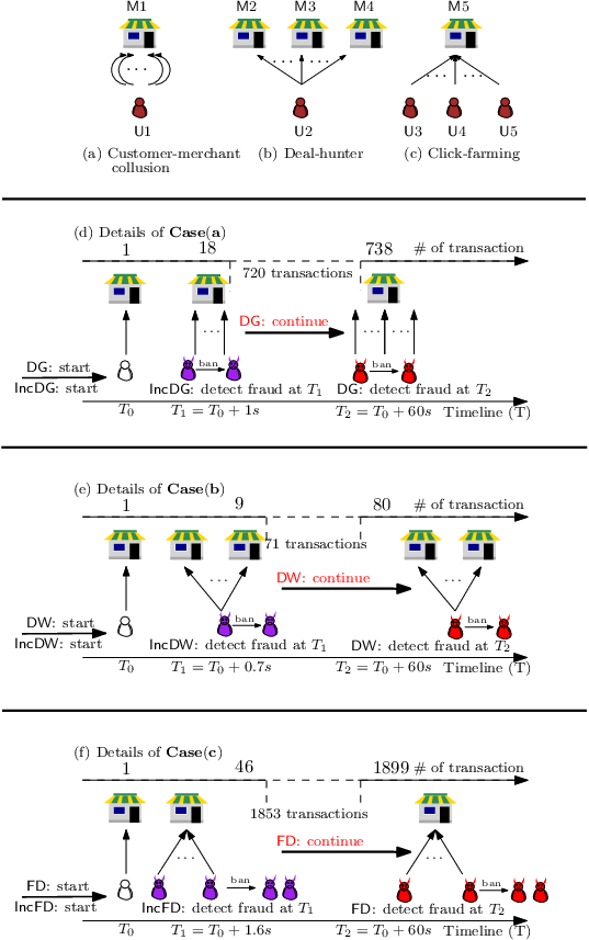
We next present the effectiveness of in discovering meaningful fraud through case studies in the datasets of . There are three popular fraud patterns as shown in Figure 13. First, customer-merchant collusion is the customer and the merchant performing fictitious transactions to use the opportunity of promotion activities to earn the bonus (Figure 13(a)). Second, there is a group of users who take advantage of promotions or merchant bugs, called deal-hunter (Figure 13(b)). Third, some merchants recruit fraudsters to create false prosperity by performing fictitious transactions, called click-farming (Figure 13(c)). All three cases form a dense subgraph in a short period of time.
Customer-merchant collusion. We detail the customer-mercant collusion in Figure 13(d). and start both at . Under the semantic of , the user becomes a fraudster at (one second after ). spots the fraudster at with negligible delay. However, cannot detect this fraud at , as it is still evaluating the graph snapshot at . By , this fraudster will be detected after the second round detection of at (about 60 seconds after ). During the time period , there are potential fraudulent transactions generated.
Deal-hunter. We investigate the details of customer-merchant collusion in Figure 13(e). and start both at . Under the semantic of , the user becomes a fraudster at ( second after ). identifies the fraudster at with negligible delay. However, cannot detect this fraud at , as it is still evaluating the graph snapshot at . By , this fraudster will be detected after the second round detection of at (about 60 seconds after ). During the time period , there are potential fraudulent transactions generated.
Click-farming. Last but not least, we present the details of click-farming in Figure 13(f). and start both at . Under the semantic of , the group of users becomes fraudsters at ( second after ). spots the fraudsters at with negligible delay. However, cannot detect this fraud at , as it is still evaluating the graph snapshot at . By , these fraudsters will be detected after the second round detection of at (about 60 seconds after ). During the time period , there are potential fraudulent transactions generated.


Consider a dense subgraph , it could consists of multiple fraud instances as shown in Figure 14. consists of , and and all of their densities are equal to . Therefore, all will be returned, since they commonly form a dense subgraph . We enumerate these instances once new fraudsters are identified.
Fraud enumeration. Figure 15 depicts the new fraudsters identified by in timespans. Once new fraudsters are detected, enumerates them and reports them to the moderators. In Figure 15, each bar represents the number of fraudulent instances are detected in the corresponding timespan. We investigated the detected fraudsters and found that most of their transactions corresponded to actual fraud, including customer-merchant collusion, deal-hunter and click-farming.
Appendix C Future extensions
We discuss a few possible extensions of our current system, including edge deletion, enumeration and fraud detection within a given period of time.
C.1. Peeling sequence reordering with edge deletion
The company will delete some outdated transactions since they are not of much value for fraud detection in some operational demands, e.g., some transactions generated several years ago. Given such an operational demand, we consider the extension of incremental maintenance with edge deletion of (without loss of generality, we assume ). A straightforward solution is also to reorder the peeling sequence. We summarize the key steps as follows and leave the extension details of in future work.
Incremental algorithm (). initializes an empty vector for the updated peeling sequence . maintains a pending queue to store the vertices pending reordering. We iteratively compare 1) the head of , denoted by and 2) the vertex in the peeling sequence , where . The corresponding peeling weights are denoted by and . We consider the following two cases.
Case 1. If the peeling weight , we insert into and update the priorities in for the neighbors of , , .
Case 2. If the peeling weight , we append to .

While is non-empty, we iteratively compare 1) the head of and 2) the vertex in the peeling sequence , where . The incremental maintenance is identical to that of edge insertion in Section 4.1. Specifically, we consider the following three cases:
Case 1. If , we pop the from and insert it to . Then we update the priorities in for the neighbors of , .
Case 2. If and or , we insert into . The peeling weight is , .
Case 3. If and and , we insert to , .
We repeat the above iteration until is empty.
Example C.0.
Consider the graph in Figure 16 and its peeling sequence . Suppose that an outdated edge is deleted from as shown in the LHS of Figure 16. The reordering procedure is presented in the RHS of Figure 16. is pushed to the pending queue . Since the peeling weights and are larger than the peeling weight of . and are inserted into . Since the peeling weight of is less than that of , it will be appended to . Similarly and are appended to accordingly. Once is empty, the rest of the vertices, and , in are appended to directly. Therefore, the reordered peeling sequence is .
C.2. Dense subgraph enumeration
In case of the enumeration of dense subgraphs due to some operational demands, we consider both static graphs and dynamic graphs.
Static graphs. Given a graph , peeling algorithm returns . To enumerate dense subgraphs, we can perform the peeling algorithm by removing from , denoted by . Specifically, and , where or . Therefore, will be returned as the second densest subgraph. We can perform the peeling algorithm recursively to enumerate all dense subgraphs.
It is remarkable that we do not have to compute from scratch. Instead, we can perform the incremental maintenance of edge deletion as introduced in Section C.1.
Dynamic graphs. Given a graph and graph updates , a straightforward solution is to reorder the peeling sequence by Algorithm 2 first. For the enumeration, we can think of this dynamic graph as a static graph.
C.3. Fraud detection during some time period
Given a graph generated during a timespan () and the peeling sequence . Taking a new graph generated during a timespan , we would like to identify the peeling sequence on , i.e., . To simply our discussion, we denote a set of edges generated during timespan by
Case 1. If or , and do not overlap. Therefore, we directly apply the peeling algorithm on .
Case 2. If and , we perform Algorithm 2 by inserting two sets of edges, and to . Then we can identify the peeling sequence on .
Case 3. If and , we perform incremental maintenance in Section C.1 by deleting two sets of edges, and from . Then we can identify the peeling sequence on .
Case 4. If , we perform Algorithm 2 by inserting a set of edges, to and perform incremental maintenance in Section C.1 by deleting a set of edges from .
Case 5. If , we perform Algorithm 2 by inserting a set of edges, to and perform incremental maintenance in Section C.1 by deleting a set of edges from .

Appendix D Accuracy guarantee of Algorithm 2
Correctness and accuracy guarantee. In Case 1, if , is chosen to insert to since it has the smallest peeling weight due to Lemma 4.3. In Case 2(b), is the smallest peeling weight and is chosen to insert to . The peeling sequence is identical to that of , since in each iteration the vertex with the smallest peeling weight is chosen. The accuracy of the worst-case is preserved due to Lemma 2.2.
Appendix E Properties of density metrics
Density metrics . We adopt the class of metrics in previous studies [19, 18, 6], , where is the total weight of , i.e., the sum of the weight of and :
| (9) |
We use to denote the total suspiciousness of the edges and to denote the total suspiciousness of , i.e.,
| (10) |
and
| (11) |
The density metric defined in Equation 9 satisfies Axiom 1-3. We adapted these basic properties from [21].
Axiom 1.
[Vertex suspiciousness] If 1) , 2) , and 3) , then .
Proof.
| (12) |
∎
With slight abuse of definition, we use to denote the total suspiciousness of on the graph .
Axiom 2.
[Edge suspiciousness] If , then .
Proof.
| (13) |
∎
Axiom 3.
[Concentration] If and , then .
Proof.
| (14) |
∎
Appendix F Instances of
We show that the popular peeling algorithms can be easily implemented and supported by , e.g., [6], [18] and [19].
Instance 1. Dense subgraphs () [6]. is designed to quantify the connectivity of substructures. It is widely used to detect fake comments [24] and fraudulent activities [3] on social graphs. Let . The density metric of is defined by . To implement on , developers only need to design and plug in the suspiciousness function by calling . Specifically, is a constant function for edges, i.e., .
Instance 2. Dense weighted subgraphs () [18]. On transaction graphs, there are weights on the edges in usual, such as the transaction amount. The density metric of is defined by , where is the weight of the edge . To implement , users only need to plug in the suspiciousness function , i.e., given an edge, .
Instance 3. Fraudar () [19]. To resist the camouflage of fraudsters, Hooi et al. [19] proposed to weight edges and set the prior suspiciousness of each vertex with side information. Let . The density metric of is defined as follows:
| (15) |
To implement on , users only need to plug in the suspiciousness function for the vertices by calling and the suspiciousness function for the edges by calling . Specifically, 1) is a constant function, i.e., given a vertex , and 2) is a logarithmic function such that given an edge , , where is the degree of the object vertex between and , and is a small positive constant [19].
Developers can easily implement customized peeling algorithms with , which significantly reduces the engineering effort. For example, users write only about lines of code (compared to about lines in the original [19]) to implement as shown in List 2. enables to be incrmental by nature. Similar observations are made in and .